
Submitted:
05 February 2025
Posted:
06 February 2025
You are already at the latest version
Abstract
Many fields or disciplines (e.g. uncertainty analysis in measurement science) require a combination of probability distributions. This paper examines three methods for combining probability distributions: weighted linear pooling, geometric pooling, and the law of combination of distributions (LCD). It provides insights into these three methods under the normality assumption. It shows that the weighted linear pooling method preserves all the variability (including heterogeneity) information in the original distributions; neither the geometric pooling method nor the LCD method preserves all the variability information, leading to information loss. We propose an index for measuring the information loss of a method with respect to the weighted linear pooling method. This paper also shows that the weighted linear pooling method can be used as an alternative to random-effects meta-analysis. Three examples are presented: the combination of two normal distributions, the combination of three discrete distributions, and the determination of the Newtonian constant of gravitation.
Keywords:
combining distributions
; gematric pooling
; linear pooling
; meta-analysis
; probability distributions
1. Introduction
The purpose of combining probability distributions is to obtain a single, refined distribution (referred to in this paper as the combined distribution) that incorporates the information about the same unknown quantity in the original distributions. The need to combine distributions arises in many fields or disciplines, including measurement science, economics, machine learning, statistics, and risk analysis. Combining distributions may be under other terminology such as aggregating distributions (e.g. Clemen & Winkler, 2007), combining expert judgments (e.g. Clemen & Winkler, 1999; McAndrew et al., 2021), conflation of probability distributions (e.g. Hill, 2011), and fusion of probability density functions (e.g. Koliander et al., 2022).
The problem of combining distributions has been reviewed by several authors, such as Genest and Zidek (1986), Ouchi (2004), McAndrew et al. (2021), and Koliander et al. (2022). In this paper, we focus on three methods: weighted linear pooling, geometric pooling, and the law of combination of distributions (LCD) (Huang, 2020). The LCD method is called the method of conflating distributions by Hill (2011). Although these three methods have been discussed in the literature, detailed and in-depth comparisons between them seem to be insufficient. In particular, no discussion on the possible information loss caused by these methods was found in the literature. This paper fills this gap.
Philosophically speaking, combining distributions is to consolidate the information from several independent sources. This is similar in nature to meta-analysis, a statistical procedure for combining the results from several independent studies (which can be represented by probability distributions). These studies often have difference in their design and conduct, leading to heterogeneous results (Langan et al., 2019). An important task in meta-analysis is to estimate the variance of heterogeneity based on the Gaussian random-effects model. This is therefore called random-effects meta-analysis. There are many statistical methods for estimating heterogeneity variance. These methods can be classified into two broad categories: closed-form (non-iterative) estimators and iterative estimators (Veroniki et al., 2016). The well-known DerSimonian–Laird (DL) method (1986) is a closed-form estimator. The Hedges and Olkin (HO) method (1985) is another closed-form estimator. The Paule-Mandel (PM) method (1982, 1989), the maximum likelihood (ML) method (e.g. Hardy & Thompson, 1996), and the restricted maximum likelihood (REML) method (e.g. Raudenbush, 2009; Viechtbauer, 2007) are well-known iterative estimators. For reviews on heterogeneity variance estimators, the interested reader is referred to Sidik and Jonkman (2007), Veroniki et al. (2016), Petropoulou and Mavridis (2017), Langan et al. (2019), and Tanriver-Ayder et al. (2021).
This study was originally designed to compare the three distribution combination methods. However, when examining the weighted linear pooling method, we found that its calculation results of heterogeneity variance were consistent with the results of random-effects meta-analysis. Therefore, we extended this study to explore the application of the weighted linear pooling method in random-effects meta-analysis.
In the following sections, section 2 describes the weighted linear pooling method and its use as an alternative to random-effects meta-analysis. Sections 3 describes the geometric pooling method. Section 4 describes the law of combination of distributions (LCD). Section 5 discusses the information loss of the geometric pooling and LCD methods. Section 6 gives three examples: two for comparing the three methods and one for random-effects meta-analysis. Sections 7 presents conclusion.
2. Weighted Linear Pooling (Method 1) and Its Use as an Alternative to Random-effects Meta-Analysis
Consider N independent distributions of a quantity Y. Each distribution has two parameters: the mean and variance . We assume that Y is normally distributed . The weighted linear pooling method gives a combined distribution of Y with the combined PDF
where is the weight that satisfies the condition . We use the inverse-variance weight. That is,
The mean of the linearly pooled distribution can be calculated as
which is the weighted-average of , the means of the original distributions.
The variance of the linearly pooled distribution can be calculated as
where
Thus,
Substituting into Equation (6) yields
where and .
It is important to note that , the weighted-average of the variances of the original distributions, can be regarded as the within-study variance in random-effects meta-analysis, and , the variance of the original distributions, can be regarded as the heterogeneity variance in random-effects meta-analysis. Thus, we can construct a normal distribution , which has the same mean and the same variance as the linearly pooled distribution. This approximate normal distribution is consistent with the result of the meta-analysis based on the Gaussian random-effects model. Therefore, the weighted linear pooling method can be taken as an alternative to random-effects meta-analysis. That is, the average effect is calculated as the inverse-variance weighted-average (inverse- WA), i.e. Equation (3), and the heterogeneity variance is calculated as
Furthermore, the heterogeneity index can be defined as
There are two advantages of using the weighted linear pooling method for random-effects meta-analysis. First, Equation (8) is a closed-form (non-iterative) estimator of the heterogeneity variance. Therefore, it is easier to implement than the commonly used iterative methods such as the Paule-Mandel (PM), maximum likelihood (ML), and restricted maximum likelihood (REML) estimators. Second, Equation (8) always gives positive values for the heterogeneity variance. In contrast, the PM, ML, and REML estimators may give negative values for the heterogeneity variance, which need to be truncated to zero.
3. Geometric Pooling (Method 2)
The geometric pooling method gives a combined distribution of Y with the combined PDF
where is the scale factor that ensures the integration of the combined distribution to be one. Note that is called the N-distribution Bhattacharyya coefficient (Kang and Wildes 2015).
Since the original distributions are assumed to be normal, i.e. , the geometrically pooled distribution is also normal. It is readily to derive that
where
and
In the special case that there are only two PDFs and , Equation (10) reduces to
Note that is called the Bhattacharyya coefficient, an index for measuring the similarity (or overlapping) between two distributions (e.g. Kang and Wildes 2015).
4. The Law of Combination of Distributions (LCD) (Method 3)
According to the law of combination of distributions (LCD), the combined PDF is the normalized product of the PDFs of the original distributions (Huang 2020). That is,
where is the scale factor that ensures the integration of to be one.
Since the original distributions are assumed to be normal, the LCD-based combined distribution is also normal. That is,
where
and
It is important to note that the LCD method is the same as the method of conflation of probability distributions discussed in Hill (2011). According to Hill and Miller (2009), “The conflation of distributions has a natural heuristic and practical interpretation – gather data from the independent laboratories sequentially and simultaneously, and record the values only when the laboratories (nearly) agree.” This means that the values that the participating laboratories disagree on are not recorded (or are ignored), resulting in a loss of information on the heterogeneity (variability) between the laboratories.
In the special case that there are only two information sources: prior and current, Equation (15) reduces to
where is the prior PDF, is the current PDF.
It is important to note that Equation (19) has the same look as the one-dimensional Bayesian theorem for continuous random variables. However, as discussed by Huang (2020), the LCD method differs from the Bayesian method in a number of aspects.
5. Information Loss of the Geometric Pooling and LCD Methods
Under the normality assumption, the means of the three combined distributions are the same, i.e. . However, the shapes of the three combined distributions are significantly different (as shown in the examples below). The linearly pooled distribution is not a Gaussian distribution; it may have heavy tails, multiple modes, and nonzero skewness (Wang & Taaffe, 2015). This is because the linearly pooled distribution takes into account all the variability in the original distributions (Clemen & Winkler, 2007). On the other hand, the geometrically pooled distribution or the LCD-based combined distribution is a Gaussian distribution, which does not take into account all the variability in the original distributions. In particular, the geometrically pooled distribution or the LCD-based combined distribution does not preserve the heterogeneity between the original distributions.
We assume that the linearly pooled distribution has no information loss. That is, the weighted linear pooling method preservers all the variability (including heterogeneity) information in the original distributions. Then, the information loss of the geometrically pooled distribution or the LCD-based combined distribution can be seen by comparing the variances of the three combined distributions. The variance of the linearly pooled distribution is , which consists of two parts: , the weighted-average of the variances of the original distributions, and , the heterogeneity variance of the original distributions. However, the variance of the geometrically pooled distribution or the LCD-based combined distribution consists of only one part: or . Neither the geometric pooling method nor the LCD method accounts for the heterogeneity between the original distributions. In other words, these two methods do not preserve all the variability information in the original distributions.
The reason why the geometric pooling method or the LCD method leads to the information loss is that its mathematical operation (average or summation) is performed in the logarithm transformed probability space. In contrast, the mathematical operation (average) of the weighted linear pooling method is performed in the original probability space. In statistics, transformation of variables or data may facilitate mathematical formulation. However, cautions should be taken when dealing with transformations that may affect the interpretation of the obtained model and subsequent statistical inference (Huang, 2018a). Harrell (2014) pointed out: “Playing with transformations distorts every part of statistical inference….”
In the logarithm transformed probability space, the geometric pooling is written as
and the LCD is written as
Note that Equation (20) is an average operation in the logarithm transformed probability space. That is, the geometric pooling method averages the Shannon information content . On the other hand, Equation (21) is a summation operation in the logarithm transformed probability space, which can be rewritten as
That is, the LCD method averages the N times the Shannon information content . This explains why the LCD-based combined distribution has a smaller variance (less than N times) than the geometrically pooled distribution.
The information loss can also be explained by considering the fact that the geometric pooling method and the LCD method only account for the overlap of the original distributions. Consider the case of two original distributions. If the two distributions do not overlap, then neither the geometrically pooled distribution nor the LCD-based combined distribution will exist because the denominator in either Equation (10) or Equation (15) will be zero. Therefore, in the special case where the two distributions do not overlap, using either of these two methods will lose all the information in the two original distributions.
We define an index for measuring the information loss of a method with respect to the weighted linear pooling method. The information loss index for the geometric pooling method is
The information loss index for the LCD method is
If the heterogeneity variance is zero, e.g. the original distributions are identical and completely overlapped, , indicating that the geometric pooling method does not lose any information. However, even if , the LCD method always lose some information.
6. Examples
6.1. Combination of Two Normal Distributions
Consider Y1 and Y2 are normally distributed: and . The PDF of Y1 is and the PDF of Y2 is .
The analytical expression for the PDF of the linearly pooled distribution is not available. The geometric pooling method gives the normal distribution , where and . If , . The LCD method gives the normal distribution , where and . If , .
Figure 1 shows the weighted PDFs of the two original distributions with , and , , and the combined PDFs based on the three methods. Figure 2 shows the weighted PDFs of the two original distributions with , and , , and the combined PDFs based on the three methods.
As can be seen from Figure 1, the linearly pooled distribution is bimodal. This is expected because the two original distributions are wildly separated: and . When the two original distributions are only slightly separated as shown in Figure 2: and , the linearly pooled distribution is unimodal. On the other hand, as can be seen from Figure 1 and Figure 2 that, the geometrically pooled distributions or the LCD-based combined distributions are unimodal, no matter how separated the two original distributions are. Note also that, the LCD-based combined distributions are narrower than the geometrically pooled distributions.
We also calculated the information loss indices for this example. The weighted-average of the variances of the two original distributions is
The heterogeneity variance is
where .
Figure 3 shows the plots of the information loss indices (for the geometric pooling method) and (for the LCD method) as a function of the difference between the means of the two original distributions with and .
As can be seen from Figure 3, the information loss index of the LCD method is always greater than that of the geometric pooling method. This is expected because the variance of the LCD-based combined distribution is always smaller than the variance of the geometrically pooled distribution. Note that as the difference between the two means increases, the information loss index also increases. This is because the heterogeneity variance increases as the difference between the two means increases.
6.2. Combination of Three Discrete Distributions
Kang and Wildes (2015) considered an example of three discrete distributions with some overlap. They showed that the overlapping regions produce a Bhattacharyya coefficient value that is greater than zero. In this study, we use their distribution data (shown in Table 1) to compare the three methods for combining distributions. For simplicity, we use the arithmetic mean in the weighted linear pooling method, which gives the combined probability mass function (PMF)
The geometric pooling method gives the combined PMF
where M is the number of bins.
The LCD method gives the combined PMF
Table 1 show the PMFs of the three original distributions and the combined PMFs obtained by the three methods.
As can be seen from Table 1, the combined PMF obtained by the geometric pooling method or the LCD method has a probability of 1 only at x=5, indicating that most of the information in the three original distributions is lost. This is because the three original distributions overlap only at x=5. In contrast, the combined PMF obtained by the weighted linear pooling method retains all the information in the three original distributions.
6.3. Determination of the Newtonian Constant of Gravitation (Random-Effects Meta-Analysis)
Given a dataset {Gi, σi} provided by participating laboratories, the Newtonian constant G can be determined using random-effects meta-analysis (e.g. Koepke et al., 2017; Willink, 2007; Mohr et al., 2016; Huang, 2018b). Huang (2023) recently analyzed two datasets: one found in Dose (2007) (referred to as the old dataset) and the other found in Koepke et al. (2017) and Mohr et al. (2016) (referred to as the new dataset), using eight random-effects methods: inverse-σ WA (WA stands for weighted-average), inverse-σ2 WA, inverse-RSE WA (RSE stands for root-squared error), DerSimonian–Laird (DL), Hedges and Olkin (HO) (i.e. arithmetic mean), Paule-Mandel (PM), maximum likelihood (ML), and restricted maximum likelihood (REML). In this example, we analyzed these two datasets using the weighted linear pooling method and compared it with these eight random-effects methods.
Tables 2 and Table 3 show the results for (estimated G), (estimated heterogeneity standard deviation), and the estimated heterogeneity index based on the old and new datasets respectively, using the weighted linear pooing method (this study) and the eight random-effects methods (Huang, 2023).

Table 2.
Results for the determination of the Newtonian constant of gravitation based on the old dataset (the unit for and is ).
Table 2.
Results for the determination of the Newtonian constant of gravitation based on the old dataset (the unit for and is ).
| Estimator |
|
|
I2 (%) |
|---|---|---|---|
| Arithmetic mean (HO) | 6.67497 | 0.00335 | 99.5 |
| Inverse-σ WA | 6.67401 | 0.00120 | 96.3 |
| Inverse-σ2 WA | 6.67419 | 0.00081 | 92.2 |
| Inverse-RSE WA | 6.67400 | 0.00088 | 93.3 |
| DerSimonian–Laird (DL) | 6.67373 | 0.00081 | 92.2 |
| Paule-Mandel (PM) | 6.67368 | 0.00131 | 96.9 |
| Maximum likelihood (ML) | 6.67369 | 0.00110 | 95.6 |
| Restricted maximum likelihood (REML) | 6.67373 | 0.00119 | 96.2 |
| Weighted linear pooling (this study) | 6.67419 | 0.00064 | 88.1 |
As can be seen from Table 2 and Table 3 that the weighted linear pooling estimates , , and I2 are consistent with those given by the eight random-effects methods. Note that, as expected, the inverse-σ2 WA and the weighted linear pooling give the same estimate .
It should be noted that the values shown in Table 2 and Table 3 are significantly different from those of Huang (2023). This is because this study uses the inverse-variance weighted-average to calculate , while Huang (2023) used the arithmetic mean . The inverse-variance weighted-average is very different from the arithmetic mean, especially for the old dataset. However, I2 is not an absolute measure of the heterogeneity between studies (Borenstein et al., 2017). The strength of the heterogeneity is measured by .
Figure 4 and Figure 5 show the combined distributions for the old and new datasets respectively. As can be seen from Figure 4 and Figure 5, the three combined distributions are significantly different. The linearly pooled distributions have heavy tails and multiple modes, while the geometrically pooled distributions and the LCD-based combined distributions are Gaussian.
7. Conclusions
The combined distributions based on the three methods (weighted linear pooling, geometric pooling, and LCD) are significantly different. The weighted linear pooling method preserves all the variability (including heterogeneity) information in the original distributions, while the geometric pooling method and the LCD method may cause serious information loss. The proposed information loss index can be used to measure the information loss. The geometric pooling method and the LCD method must be used with caution in practical applications.
The normal approximation of the linearly pooled distribution is consistent with the results of random-effects meta-analysis. Therefore, the weighted linear pooling method can be used as an alternative to random-effects meta-analysis. One of the advantages of using the weighted linear pooling method is that it a closed-form (non-iterative) method for estimating the heterogeneity variance. Another advantage is that it always gives positive values for the heterogeneity variance. Further research is needed to examine the performance of the weighted linear pooling method for random-effects meta-analysis.
References
- Borenstein M, Higgins J P T, Larry V, Hedges L V, and Rothstein H R 2017 Basics of meta-analysis: I2 is not an absolute measure of heterogeneity Research Synthesis Methods. [CrossRef]
- Clemen R T and Winkler R L 1999 Combining probability distributions from experts in risk analysis Risk Anal 19 187–203. [CrossRef]
- Clemen R T and Winkler R L 2007 Aggregating probability distributions In W. Edwards, R. F. Miles, Jr., & D. von Winterfeldt (Eds.) Advances in decision analysis: From foundations to applications (pp. 154–176), Cambridge University Press. [CrossRef]
- DerSimonian R and Laird N 1986 Meta-analysis in clinical trials Controlled Clinical Trials 7(3) 177–188. [CrossRef]
- Dose V 2007 Bayesian estimate of the Newtonian constant of gravitation Measurement Science and Technology 18(1) 176-182.
- Genest C and Zidek J V 1986 Combining probability distributions: a critique and an annotated bibliography Statistical Science 1(1) 114-135.
- Hardy R J and Thompson S G 1996 A likelihood approach to meta-analysis with random effects. Statistics in Medicine 15(6) 619–629. [CrossRef]
- Harrell F 2014 Comments on: ‘Pitfalls to avoid when transforming data?’ Cross Validated, http://stats.stackexchange.com/questions/90149/pitfalls-to-avoid-when-transforming-data.
- Hedges L V and Olkin I 1985 Statistical methods for meta-analysis San Diego, CA: Academic Press.
- Hill T P 2011 Conflations of probability distributions Transactions of the American Mathematical Society 363(6) 3351–3372 http://www.jstor.org/stable/23032795.
- Hill T P and Miller J 2009 An optimal method to combine results from different experiments arXiv: Data Analysis, Statistics and Probability arXiv:0901.4957.
- Huang H 2018a Uncertainty estimation with a small number of measurements, Part I: new insights on the t-interval method and its limitations Measurement Science and Technology 29(1) 015004. [CrossRef]
- Huang H 2018b A new method for estimating consensus value in interlaboratory comparison. Metrologia 55(1) 106-113. [CrossRef]
- Huang H 2020 Two simple and practical frequentist methods for combining prior information with current measurement in uncertainty analysis Cal Lab the International Journal of Metrology 27(3) 22-32 available from ResearchGate: https://www.researchgate.net/publication/344502279_Two_simple_and_practical_methods_for_combining_prior_information_with_current_measurement_in_uncertainty_analysis.
- Huang H 2023 Combining estimators in interlaboratory studies and meta-analyses Research Synthesis Methods. [CrossRef]
- Kang S and Wildes R P 2015 The n-distribution Bhattacharyya coefficient Technical Report EECS-2015-02, York University, Toronto, Ontario, Canada https://www.eecs.yorku.ca/research/techreports/2015/EECS-2015-02.pdf.
- Koepke A, Lafarge T, Possolo A and Toman B 2017 Consensus building for interlaboratory studies, key comparisons, and meta-analysis Metrologia 54(3) S34–S62.
- Koliander G, El-Laham Y, Djurić P M, and Hlawatsch F 2022 Fusion of probability density functions, in Proceedings of the IEEE 110(4) 404-453. [CrossRef]
- Langan D, Higgins J P T, Jackson D, Bowden J, Veroniki A A, Kontopantelis E, Viechtbauer W, and Simmonds M 2019 A comparison of heterogeneity variance estimators in simulated random-effects meta-analyses Research Synthesis Methods 10(1) 83-98. [CrossRef]
- Mathoverflow 2022 How close are two Gaussian random variables? URL (version: 2022-04-30): https://mathoverflow.net/q/421397 accessed November 2023.
- McAndrew T, Wattanachit N, Gibson G C, and Reich N G 2021 Aggregating predictions from experts: a review of statistical methods, experiments, and applications Wiley Interdiscip Rev Comput Stat. 13(2):e1514. Epub 2020 Jun 16. PMID: 33777310; PMCID: PMC7996321. [CrossRef]
- Mohr P J, Newell D B, and Taylor B N 2016 CODATA recommended values of the fundamental physical constants: 2014 Reviews of Modern Physics 88 035009.
- Ouchi F 2004 A literature review on the use of expert opinion in probabilistic risk analysis (English) Policy, Research working paper; no. WPS 3201 Washington, D.C.: World Bank Group.http://documents.worldbank.org/curated/en/346091468765322039/A-literature-review-on-the-use-of-expert-opinion-in-probabilistic-risk-analysis.
- Paule R C and Mandel J 1982 Consensus values and weighting factors Journal of Research of the National Bureau of Standards 87(5) 377–385.
- Paule R C and Mandel J 1989 Consensus values, regressions, and weighting factors Journal of Research of the National Institute of Standards and Technology 94(3) 197-203.
- Petropoulou M and Mavridis D A 2017 Comparison of 20 heterogeneity variance estimators in statistical synthesis of results from studies: A simulation study Wiley Statistics in Medicine, 36(27) 4266-4280. [CrossRef]
- Raudenbush S W 2009 Analyzing effect sizes: random-effects models. In Cooper, H., Hedges, L. V., & Valentine, J. C. (eds.), The Handbook of Research Synthesis and Meta-Analysis (pp. 295–315), New York: Russell Sage Foundation.
- Sidik K and Jonkman J N 2007 A comparison of heterogeneity variance estimators in combining results of studies Statistics in Medicine 26(9) 1964-1981. [CrossRef]
- Tanriver-Ayder E, Faes C, van de Casteele T, McCann S K, and Macleod M R 2021 Comparison of commonly used methods in random effects meta-analysis: application to preclinical data in drug discovery research BMJ Open Science 5:e100074. [CrossRef]
- Veroniki A A, Jackson D, Viechtbauer W, Bender R, Bowden J, Knapp G, Kuss O, Higgins J P T, Langan D, and Salanti G 2016 Methods to estimate the between-study variance and its uncertainty in meta-analysis Res Synth Methods 7(1) 55–79. [CrossRef]
- Viechtbauer W 2007 Confidence intervals for the amount of heterogeneity in meta-analysis Statistics in Medicine 26(1) 37–52.
- Wang J and Taaffe M R 2015 Multivariate mixtures of normal distributions: properties, random vector generation, fitting, and as models of market daily changes INFORMS J. Comput. 27(2) 193–203.
- Willink R 2007 Comments on ‘Bayesian estimate of the Newtonian constant of gravitation’ with an alternative analysis Measurement Science and Technology 18(7) 2275-2280.
Figure 1.
The weighted PDFs of the two original distributions with , and , , and the combined PDFs based on the three methods.
Figure 1.
The weighted PDFs of the two original distributions with , and , , and the combined PDFs based on the three methods.
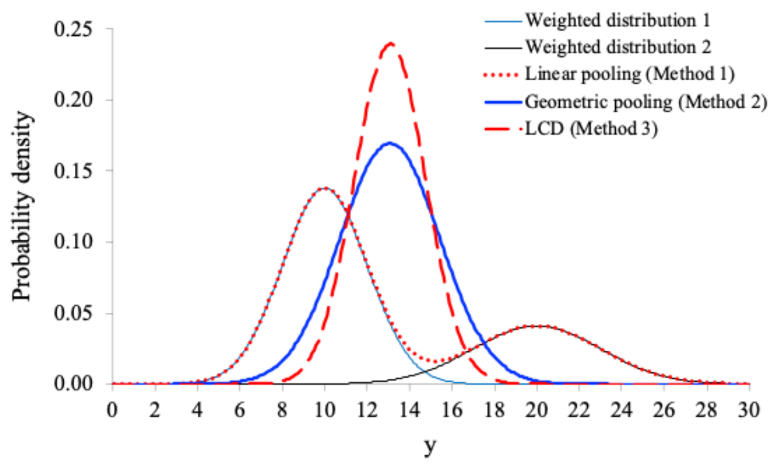
Figure 2.
The weighted PDFs of the two original distributions with , and , and the combined PDFs based on the three methods.
Figure 2.
The weighted PDFs of the two original distributions with , and , and the combined PDFs based on the three methods.
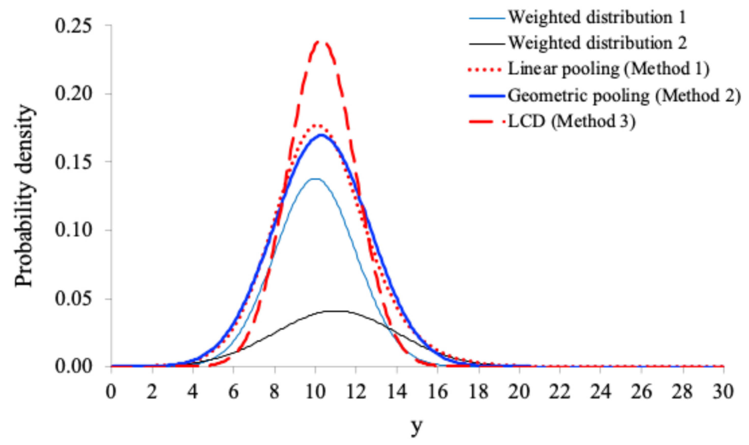
Figure 3.
The information loss indices (for the geometric pooling method) and (for the LCD method) as a function of the difference between the means of the two original distributions with and .
Figure 3.
The information loss indices (for the geometric pooling method) and (for the LCD method) as a function of the difference between the means of the two original distributions with and .
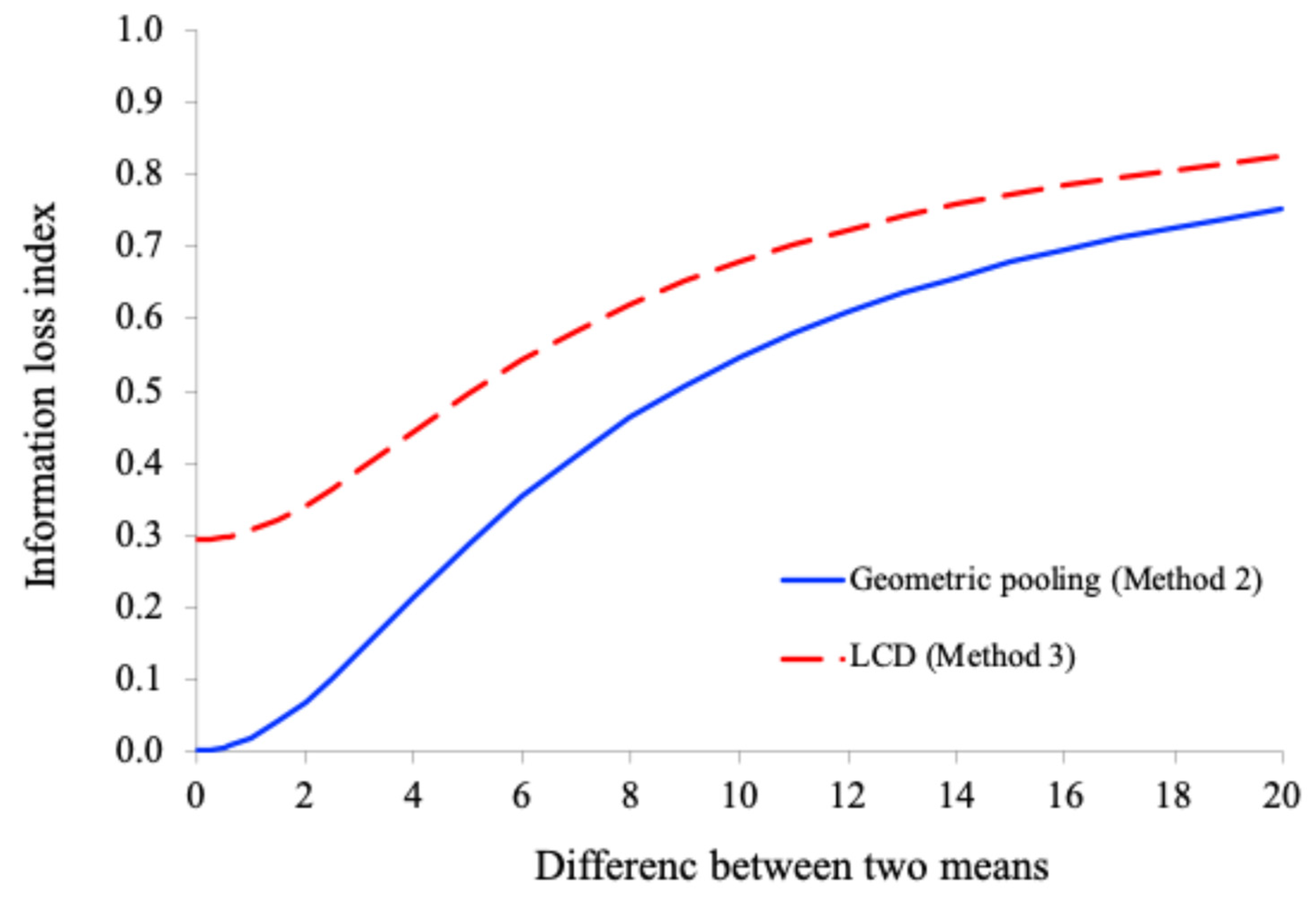
Figure 4.
Combined distributions for the old dataset.
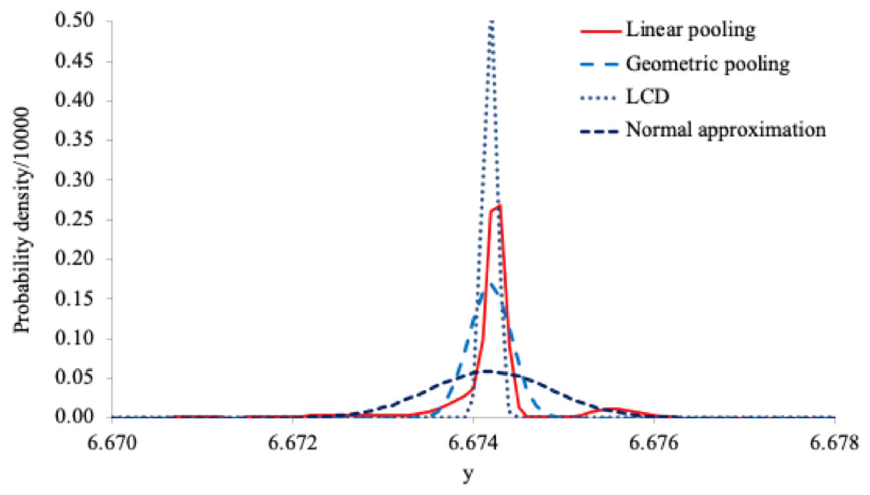
Figure 5.
Combined distributions for the new dataset.
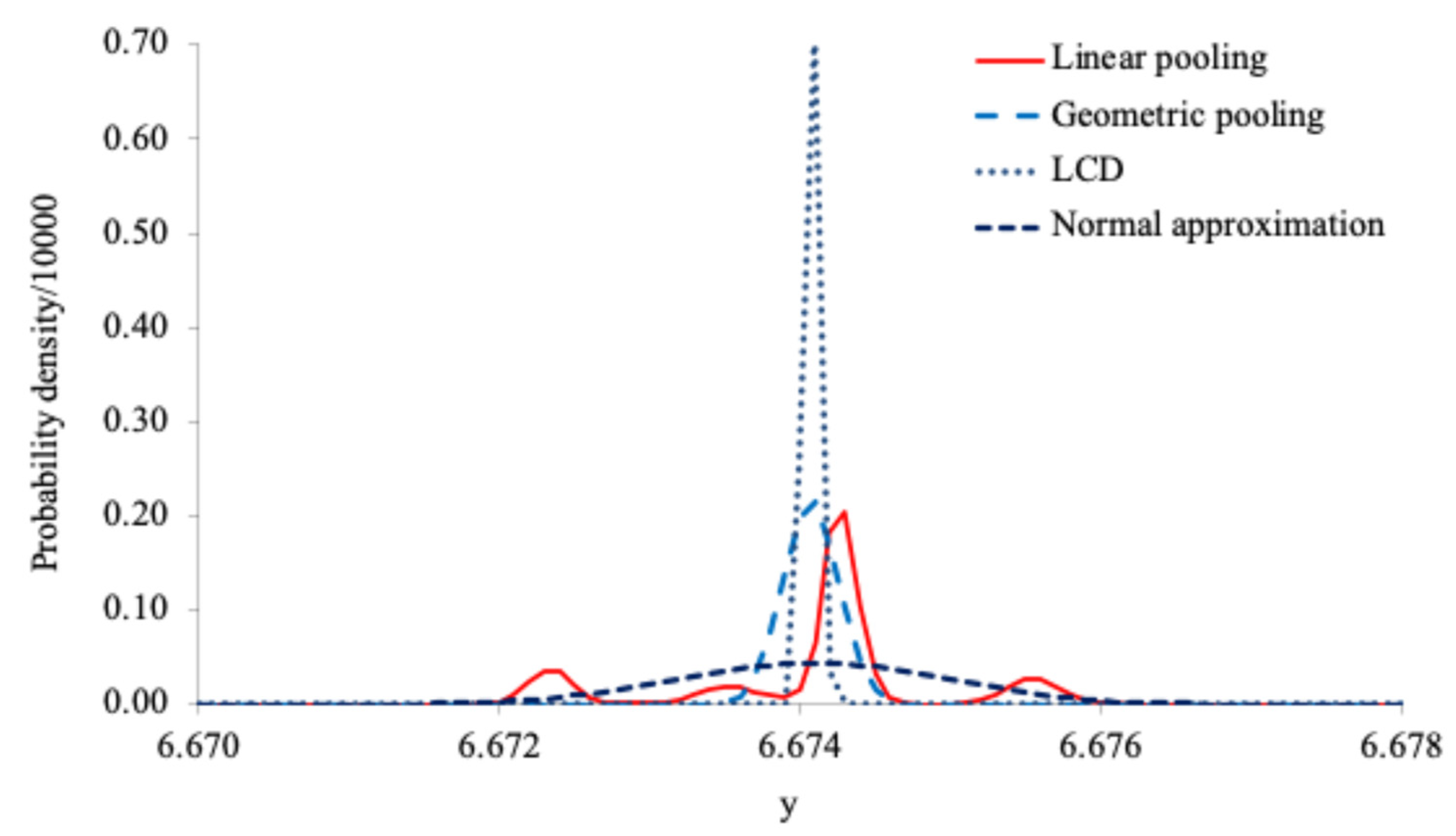
Table 1.
The PMFs of three original distributions and the combined PMFs obtained by the three methods.
Table 1.
The PMFs of three original distributions and the combined PMFs obtained by the three methods.
| x | P1(x) | P2(x) | P3(x) | PL(x) | PG(x) | PLCD(x) |
|---|---|---|---|---|---|---|
| 0 | 0 | 0 | 0 | 0 | 0 | 0 |
| 1 | 0 | 0 | 0 | 0 | 0 | 0 |
| 2 | 0.01 | 0 | 0 | 0.003 | 0 | 0 |
| 3 | 0.04 | 0.15 | 0 | 0.063 | 0 | 0 |
| 4 | 0.25 | 0.7 | 0 | 0.317 | 0 | 0 |
| 5 | 0.4 | 0.15 | 0.15 | 0.233 | 1 | 1 |
| 6 | 0.25 | 0 | 0.7 | 0.317 | 0 | 0 |
| 7 | 0.05 | 0 | 0.15 | 0.067 | 0 | 0 |
| 8 | 0 | 0 | 0 | 0 | 0 | 0 |
| 9 | 0 | 0 | 0 | 0 | 0 | 0 |
| 10 | 0 | 0 | 0 | 0 | 0 | 0 |
Table 3.
Results for the determination of the Newtonian constant of gravitation based on the new dataset (the unit for and is ).
Table 3.
Results for the determination of the Newtonian constant of gravitation based on the new dataset (the unit for and is ).
| Estimator |
|
|
I2 (%) |
|---|---|---|---|
| Arithmetic mean (HO) | 6.67367 | 0.00104 | 96.9 |
| Inverse-σ WA | 6.67397 | 0.00102 | 96.8 |
| Inverse-σ2 WA | 6.67408 | 0.00095 | 96.4 |
| Inverse-RSE WA | 6.67385 | 0.00071 | 93.7 |
| DerSimonian–Laird (DL) | 6.67378 | 0.00095 | 96.4 |
| Paule-Mandel (PM) | 6.67376 | 0.00129 | 98.0 |
| Maximum likelihood (ML) | 6.67378 | 0.00102 | 96.8 |
| Restricted maximum likelihood (REML) | 6.67377 | 0.00107 | 97.1 |
| Weighted linear pooling (this study) | 6.67408 | 0.00088 | 95.8 |
Disclaimer/Publisher’s Note: The statements, opinions and data contained in all publications are solely those of the individual author(s) and contributor(s) and not of MDPI and/or the editor(s). MDPI and/or the editor(s) disclaim responsibility for any injury to people or property resulting from any ideas, methods, instructions or products referred to in the content. |
© 2025 by the author. Licensee MDPI, Basel, Switzerland. This article is an open access article distributed under the terms and conditions of the Creative Commons Attribution (CC BY) license (https://creativecommons.org/licenses/by/4.0/).
Copyright: This open access article is published under a Creative Commons CC BY 4.0 license, which permit the free download, distribution, and reuse, provided that the author and preprint are cited in any reuse.


