
Submitted:
04 February 2025
Posted:
06 February 2025
You are already at the latest version
Abstract
Clustering high-dimensional and structural data remains a key challenge in computational biology, especially for complex single-cell and multi-omics datasets. In this study, we present $K$-volume clustering, a novel algorithm that uses the total convex volume defined by points within a cluster as a biologically relevant and geometrically interpretable criterion. This method simultaneously optimizes both the hierarchical structure and the number of clusters at each level through nonlinear optimization. Validation on real datasets shows that $K$-volume clustering outperforms traditional methods across a range of biological applications. With its theoretical foundation and broad applicability, $K$-volume clustering holds great promise as a core tool for diverse data analysis tasks.
Keywords:
single-cell omics
; clustering algorithms
; gene regulatory networks
1. Introduction
Clustering is a fundamental task in data analysis, aiming to group similar data points based on their intrinsic properties and patterns, without relying on labeled data [1]. Among the various clustering methods, K-means and its variants are widely recognized for their simplicity, scalability, and efficiency [2,3]. The K-means algorithm partitions a dataset into K clusters by iteratively minimizing intra-cluster variance and maximizing inter-cluster separation. Variants such as K-center [4], K-median [5], and K-density [6] have been introduced to better handle diverse data distributions, improve robustness to outliers, and capture nonlinear relationships. However, these methods typically require the number of clusters, K, to be predefined, which presents a significant challenge, especially with complex datasets.
Clustering methods have become essential tools in biological data analysis, particularly with the rise of high-throughput, high-dimensional datasets like single-cell RNA sequencing (scRNA-seq)[7]. scRNA-seq provides a powerful means of analyzing gene expression at the single-cell level, enabling the identification of diverse cell types, states, and lineages. In this context, clustering is critical for grouping cells with similar expression profiles to uncover cell heterogeneity and infer biological functions[8,9]. Methods such as K-means, hierarchical clustering, and graph-based clustering have been adapted to handle the high dimensionality and sparsity of scRNA-seq data [7]. Advanced variations, including those that integrate dimensionality reduction techniques like PCA or t-SNE, have further enhanced the interpretability of scRNA-seq clusters, facilitating the discovery of novel cell populations and their functional characteristics [10].
Identifying the optimal number of clusters (K) and defining hierarchical layers (H) remain significant challenges in both theoretical analysis and practical applications [3]. In K-means clustering, the need to predefine K can lead to complications, as improper choices may result in over- or under-clustering, distorting the underlying data structure. Similarly, hierarchical clustering lacks a universal criterion for determining the appropriate number of layers or meaningful cut points in the dendrogram, which can lead to subjective or inconsistent interpretations [11]. Approaches like the elbow method [12], silhouette analysis [13], and gap statistics [14] have been developed to estimate K, but these techniques are often computationally expensive and highly sensitive to dataset characteristics. This challenge is particularly pronounced in scRNA-seq data, where the biological processes often span multiple scales and resolutions [15]. Moreover, the number of clusters can vary based on the specific objectives—whether identifying common cell populations or detecting rare cell types [7,9]. The hierarchical relationships between cell populations, shaped by lineage progression and differentiation pathways, further complicate the analysis [16,17]. Thus, there is an urgent need for robust, automated approaches that can simultaneously determine cluster numbers and uncover hierarchical structures, particularly for the complex and high-dimensional nature of scRNA-seq data.
In this study, we introduce K-volume clustering, a novel and foundational algorithm for optimal hierarchical clustering. The algorithm optimizes both the number of hierarchical layers, H, and the number of clusters, K, within each layer using nonlinear optimization principles (see Figure 1). At each level, it maximizes the difference between the area of the convex hull encompassing all sample points and the cumulative areas of the K sub-convex hulls. By jointly optimizing H and K, this method effectively determines the optimal hierarchical structure, yielding a robust clustering solution.
1.1. Related Work
Clustering partitions data points into subsets, where each subset forms a cluster based on a specified criterion [1]. Clustering algorithms group ‘similar’ data points to uncover relationships among them. Common similarity measures include Euclidean distance [18], squared Euclidean distance [19,20], and Hamming distance [21].
Clustering algorithms are generally categorized into center-based clustering and density-based clustering. Our K-volume clustering method integrates aspects of both approaches. Table 1 summarizes widely used clustering algorithms, with entries marked by * denoting our contributions in this paper. Notably, center-based clustering problems are NP-hard, and finding optimal K-means clusters remains NP-hard, even in two-dimensional space [22]. Table 1 also lists the most recent approximation algorithms for these clustering problems.
1.2. Our Contribution and Paper Organization
In this paper, we develop algorithms specifically for clustering biological data, such as cell data and single-cell omics. In particular, we propose a novel clustering algorithm that uses the total convex volume enclosed by points within the same cluster as a clustering measure.
2. A Greedy K-Volume Clustering Algorithm
We consider a clustering problem with the following input: a set of N data points, , where each point is represented as a D-dimensional integer vector in . The distance between any two points, and , is denoted by .
To evaluate clustering algorithms, we introduce a new measure based on convex volume. Specifically, the clustering cost is defined as the minimal convex volume enclosing all points within a cluster. Under this definition, a single data point has a volume of 0, and any set of collinear points also has a volume of 0.
We define the problem of partitioning data into K clusters within a hierarchical structure while minimizing the total convex volume as the K-volume clustering problem. When the dimensionality is , we refer to it as the K-area clustering problem.
2.1. The Algorithm’s Idea
We propose a simple yet elegant algorithm based on a greedy approach. In this work, we illustrate the idea for the case where , with the approach being naturally extendable to higher dimensions (). The algorithm starts with the convex hull of the data points. The key idea is to partition a cluster into two in such a way that the convex volume of the remaining clusters is minimized. This process is repeated iteratively until the total number of clusters reaches the specified value K or the given maximal hierarchical level H.
Given a set of points, finding the initial convex hull takes time [25]. The main algorithmic challenges in finding K-volume clusters are: how to partition the data points into K clusters, and how to calculate the total volume of these clusters.
Consider a set of N points, , where each point is described by its coordinates in 2D space. Without loss of generality, we assume all x-axis and y-axis values are non-negative. Our goal is to partition the points into K clusters, i.e., K convex areas on the 2D plane, such that the total area is minimized. Let S represent a set of points, and denote the area of the convex polygon enclosing S.
The algorithm proceeds as follows: Initially, using Graham’s scan [26], we calculate the convex polygon for all N points. If , this convex polygon is the optimal solution, and all points belong to the same cluster. If , we proceed to build a tree that represents the set of clusters created during the execution of the algorithm. The tree structure allows the algorithm to efficiently organize and partition the data into meaningful groups. Since each layer in the tree represents a finer partitioning, the algorithm benefits from the hierarchical structure when it comes to refining clusters, especially as the number of clusters increases. The tree has the following properties:
- The root node represents the initial convex polygon for all the data points.
- Each node in the tree corresponds to a cluster. The root of each subtree represents the cluster for all the data points clustered in its subtree.
- The leaf nodes represent the set of clusters that we currently have at any point in time.
For , we iteratively partition one of the current clusters, say C, into two subclusters, and . These subclusters, and , become the children of node C. This partitioning process continues until we have exactly K clusters or reach the maximal hierarchical level H.
When partitioning a cluster C into two subclusters and , we use a greedy approach that maximizes the size of the removed area, ensuring an optimal division.
2.2. The Algorithm’s Description
The algorithm is described in detail as follows. Consider the set C. If C is partitioned into two convex polygons, and , we observe that and do not overlap, and there must exist a straight line , defined by two points a and b, that separates and . We maintain the points of C in two lists: , the set of points defining the convex polygon, and , the set of points in the interior of the convex polygon. The algorithm consists of three steps:
-
Identify the straight lines that can separate a cluster C.Given the convexity requirements for the clusters after any partitioning, any partition of the set C into two convex polygons and can be achieved by introducing a straight line that crosses two points from the set . Given two points and , the line is defined by the equationwhich simplifies toIn total, there are such straight lines that can partition the cluster C.
-
Given a convex polygon C and a straight line , calculate the two convex polygons and separately by using Graham’s scan algorithm [26]This line partitions C into two sets and , where and . These sets are defined as follows:Due to the convexity of C, , and , we also have the following relationship:After partitioning the set C using the line into the point sets and , we construct convex polygons for each set using Graham’s scan algorithm [26]. This process results in sets , . , and . Additionally, we index the points in these sets in a clockwise order for the next step.
-
Calculate the area of a convex polygon . Then, determine the maximum area that can be removed by a single partition of the cluster.Consider the point and label the points clockwise on the convex polygon C. Using the Shoelace formula [27], the area of the convex polygon defined by the points , , …, is given byFor each line , we calculate the convex polygons resulting from the partition of the convex polygon C. Then, we compute the value . The best straight line is chosen to minimize the maximum area removed by partitioning the set C.
In Algorithm 1, we present the K-Area Clustering algorithm, denoted as K-AC, for clustering biological data. This algorithm partitions N data points into at most K clusters, C, or organizes them into at most H hierarchical levels of clusters.
| Algorithm 1:K-AC: K-area clustering algorithm(N, C, K, H) |
|
Below, We present the running time complexity of K-AC in Theorem 1.
Theorem 1.
The K-AC algorithm runs in time.
Proof.
Using Graham’s scan algorithm, line 1 of K-AC runs in time. Lines 2 and 3 take constant time. The WHILE loop runs for K rounds. In each round, we identify straight lines, where . For each straight line, it takes linear time to locate and using Equations 1,2, and . The area calculations require time. Identifying the best partition to reduce the total area size takes time on lines 10 and 11. Line 12 takes constant time, while Line 13 takes time. Updating the clusters in line 14 takes time, using Graham’s scan algorithm. Thus, the total running time of the WHILE loop is
Inequality 5 holds by Jensen’s inequality, and Equation holds under the assumption that . □
3. Experiments
In this section, we conduct experiments to evaluate our K-AC algorithm. Using biological data, we compare K-area clustering with other well-known clustering algorithms, including K-center, K-median, and K-means clustering.
3.1. Datasets
The optimal number of clusters is determined based on the true labels of the cells’ gene expression profiles.

Table 2.
Datasets that we use for experimental study of clustering algorithms
| Name | Size (# of cells) | : # of optimal clusters |
| Biase | 49 | 3 |
| Deng | 268 | 10 |
| Goolam | 124 | 5 |
| Ting | 149 | 7 |
| Yan | 90 | 7 |
3.2. Metrics
We set for the Biase, Deng, Goolam, Ting, and Yan datasets, respectively. We then measure the cost of the following clustering algorithms: the K-center clustering algorithm [27], the K-median clustering algorithm [28], the K-means Lloyd’s clustering algorithm [20], and our proposed K-area clustering algorithm K-AC. To evaluate the performance of these clustering algorithms, we use Normalized Mutual Information (NMI) [29] to assess the quality of the generated clusters.
NMI is a widely used metric for evaluating clustering performance by measuring the mutual dependence between the true labels and the predicted clusters. The mutual information is normalized to ensure values between 0 and 1, where 1 indicates perfect clustering and 0 implies no mutual information between the clustering and ground truth. The NMI between two cluster assignments C (ground truth) and (predicted clusters) is computed as:
where is the mutual information between C and , and are the entropy of C and respectively.
3.3. K-Center Clustering Algorithm
The K-center clustering algorithm aims to find a partition of the data points into K clusters, with corresponding centers such that the maximum distance between any data point and the center of its assigned cluster is minimized. Specifically, the goal is to minimize:
When K is not a fixed input or may vary as a function of the number of data points N, this K-center clustering problem becomes NP-hard. In our experiments, we apply the farthest-traversal algorithm to solve the K-center problem and generate clusters. The resulting clustering is shown in Figure 7, Figure 8, Figure 9, Figure 10 and Figure 11.
3.4. K-Median Clustering Algorithm
The K-median clustering algorithm seeks to find a partition of the data points into K clusters, with corresponding centers to minimize the total distance between each data point and the center of its assigned cluster. Specifically, the objective is to minimize:
When K is not part of an input of may be a function of n, then this K-median clustering problem is NP-hard. In our experiments, we run the Lloyd-style iteration algorithm [30] for the K-median clustering problem to generate clusters. The resulting clustering is shown in Figure 12, Figure 13, Figure 14, Figure 15 and Figure 16.
3.5. K-Means Clustering Algorithm
The K-means clustering algorithm aims to find a partition of the data points into K clusters, with corresponding centers such that the sum of squared distances between each data point and the center of its assigned cluster is minimized. Specifically, the objective is to minimize
When K is not part of an input of may be a function of n, then this K-means clustering problem is NP-hard. In our experiments, we run Llyod’s algorithm [20] for the K-means clustering problem to generate clusters. The resulting clustering is shown in Figure 17, Figure 18, Figure 19, Figure 20 and Figure 21.
3.6. K-Area Clustering Algorithm
The K-area clustering algorithm aims to find a partition of the data points into K clusters such that the sum of convex hull areas is minimized. Specifically, the objective is to minimize
where denotes the area of the region defined by the polygon .
3.7. Comparison
We summarize the NMI scores for these algorithms in Table 3. Our algorithm, K-AC, outperforms all other algorithms in three cases but is slightly less effective in two: the K-median algorithm on the Deng dataset and on the Ting dataset. This result underscores that K-AC offers a biologically relevant and geometrically interpretable clustering criterion, enabling more meaningful clusterings of high-dimensional biological data compared to the other three algorithms.
We also report the convex areas produced by these four clustering algorithms in Table 4. It is evident that the K area algorithm results in the smallest convex area, and in some cases, such as the Goolam dataset, it reduces the space by up to 60%. The comparison results are visualized in Figure 27 and Figure 28.
3.8. Hierarchical Clustering
To demonstrate the effectiveness of the K-area algorithm in interpreting the hierarchical structure of biological data—particularly in identifying the number of natural clusters—we conducted experiments to explore the construction of the cluster tree. We use the ratio of the convex hull areas between two neighboring rounds as a criterion for determining when to halt the partitioning of existing clusters.
The dataset Yan used in our experiments has an optimal number of clusters, . We calculate the total cluster areas for and summarize the results in Table 5, with visualizations in Figure 29. The area ratio between two neighboring rounds increases from 0 to 1. As the ratio approaches 1, the benefit of further partitioning into additional clusters diminishes. Notably, after , the area ratio stabilizes near 1, indicating that further partitioning yields diminishing returns. This feature of the K-area algorithm aids in identifying an appropriate value for K, the number of clusters.
We construct the cluster tree generated by the K-area algorithm to visually represent its progression from Figure 30, Figure 31, Figure 32, Figure 33, Figure 34, Figure 35 and Figure 36. The tree structure of the partitions is shown in Figure 37. In this tree, the root node represents the initial convex hull, with each parent node (a cluster) being divided into two child nodes (subclusters). The leaves of the tree correspond to the final set of clusters. The height of the tree is constrained by the given hierarchical level H.
4. Conclusion and Future Work
In this paper, we addressed the challenge of clustering biological data by developing a novel algorithm based on the total convex volume encompassed by points within the same cluster. This approach offers a biologically relevant and geometrically interpretable clustering criterion, enabling more meaningful groupings of high-dimensional biological data. We introduced the K-volume algorithm, which effectively balances accuracy and computational feasibility. Experimental evaluations demonstrated the algorithm’s effectiveness compared to well-established clustering methods, showing promising results in capturing biological structures and relationships within the data.
A key innovation of the K-volume algorithm is its ability to simultaneously optimize both the hierarchical structure and the number of clusters at each level, leveraging nonlinear optimization. Unlike traditional clustering methods, which require a predefined number of clusters, our method dynamically determines the optimal number of clusters and hierarchical layers based on the convex volume distribution. This adaptive nature makes it particularly well-suited for complex biological datasets, such as scRNA-seq and spatial transcriptomics, where cell populations exhibit multi-scale hierarchical relationships.
Moreover, the flexibility of our method extends beyond biological applications, making it a powerful tool for a wide range of data-intensive domains, including finance, social network analysis, and image segmentation, where hierarchical patterns naturally emerge. The method holds significant potential as a core component in modern data analysis pipelines. By integrating this method into widely used computational frameworks, we envision it becoming a standard clustering technique for high-dimensional and hierarchical data, offering a versatile and scalable solution for data-driven discovery.
Looking ahead, future research will focus on extending this framework by incorporating advanced high-dimensional data processing techniques, such as dimensionality reduction methods and deep learning-based feature extraction, to further enhance clustering performance [31,32]. We also plan to integrate multi-omics data, including single-cell spatial transcriptomics [33], epigenomics [34], and proteomics [35], to create a more holistic representation of cellular states and regulatory mechanisms. By combining these advancements, we aim to develop a powerful, scalable clustering framework capable of uncovering complex biological patterns across multiple layers of molecular information, ultimately contributing to a deeper understanding of cellular functions and disease mechanisms.
Author Contributions
Conceptualization, Yong Chen and Fei Li; methodology, Yong Chen and Fei Li; software, Fei Li; validation, Yong Chen and Fei Li; formal analysis, Fei Li; resources, Yong Chen and Fei Li; data curation, Yong Chen; writing—original draft preparation, Fei Li; writing—review and editing, Yong Chen; visualization, Yong Chen and Fei Li; supervision, Yong Chen and Fei Li; project administration, Yong Chen and Fei Li; funding acquisition, Yong Chen. All authors have read and agreed to the published version of the manuscript.
Funding
This work was supported by the NSF CAREER Award DBI-2239350.
Data Availability Statement
The research data is stored at https://drive.google.com/drive/folders/1OJdP3UjZKXrvFx4QsIyhG1-l7LX2Tikc?usp=sharing. The code is available at GitHub https://github.com/aqcc-va/clustering.
Conflicts of Interest
The authors declare no conflicts of interest.
References
- Blum, A.; Hopcroft, J.; Kannan, R. Foundations of Data Science; Cambridge University Press, 2020.
- Ahmed, M.; Seraj, R.; Islam, S.M.S. The k-means Algorithm: A Comprehensive Survey and Performance Evaluation. Electronics 2020, 9. [Google Scholar] [CrossRef]
- Ikotun, A.M.; Ezugwu, A.E.; Abualigah, L.; Abuhaija, B.; Heming, J. K-means clustering algorithms: A comprehensive review, variants analysis, and advances in the era of big data. Information Sciences 2023, 622, 178–210. [Google Scholar] [CrossRef]
- Gonzalez, T.F. Clustering to minimize the maximum intercluster distance. Theoretical Computer Science 1985, 38, 293–306. [Google Scholar] [CrossRef]
- Byrka, J.; Pensyl, T.; Rybicki, B.; Srinivasan, A.; TrinhAuthors, K. An Improved Approximation for k-Median and Positive Correlation in Budgeted Optimization. ACM Transactions on Algorithms (TALG) 2017, 13, 1–31. [Google Scholar] [CrossRef]
- Kumar, A.; Kumar, A.; Mallipeddi, R.; Lee, D.G. High-density cluster core-based k-means clustering with an unknown number of clusters. Applied Soft Computing 2024, 155, 111419. [Google Scholar] [CrossRef]
- Nie, X.; Qin, D.; Zhou, X.; Duo, H.; Hao, Y.; Li, B.; zhao Liang, G. Clustering ensemble in scRNA-seq data analysis: Methods, applications and challenges. Computers in biology and medicine 2023, 159, 106939. [Google Scholar] [CrossRef]
- Jovic, D.; Liang, X.; Zeng, H.; Lin, L.; Xu, F.; Luo, Y. Single-cell RNA sequencing technologies and applications: A brief overview. Clinical and Translational Medicine 2022, 12, e694. [Google Scholar] [CrossRef]
- Nossier, M.; Moussa, S.M.; Badr, N.L. Single-Cell RNA-Seq Data Clustering: Highlighting Computational Challenges and Considerations. 2023 IEEE International Conference on Bioinformatics and Biomedicine (BIBM) 2023, 4228–4234. [Google Scholar]
- Zhang, S.; Li, X.; Lin, Q.; chun Wong, K. Review of single-cell RNA-seq data clustering for cell-type identification and characterization. RNA 2020, 29, 517–530. [Google Scholar] [CrossRef]
- Ran, X.; Xi, Y.; Lu, Y.; Wang, X.; Lu, Z. Comprehensive survey on hierarchical clustering algorithms and the recent developments. Artif. Intell. Rev. 2022, 56, 8219–8264. [Google Scholar] [CrossRef]
- Marutho, D.; Hendra Handaka, S.; Wijaya, E.; Muljono. The Determination of Cluster Number at k-Mean Using Elbow Method and Purity Evaluation on Headline News. In Proceedings of the 2018 International Seminar on Application for Technology of Information and Communication, 2018, pp. 533–538. [CrossRef]
- Shutaywi, M.; Kachouie, N.N. Silhouette Analysis for Performance Evaluation in Machine Learning with Applications to Clustering. Entropy 2021, 23. [Google Scholar] [CrossRef]
- Tibshirani, R.; Walther, G.; Hastie, T. Estimating the Number of Clusters in a Data Set Via the Gap Statistic. Journal of the Royal Statistical Society Series B: Statistical Methodology 2002, 63, 411–423. [Google Scholar] [CrossRef]
- Yu, L.; Cao, Y.; Yang, J.Y.H.; Yang, P. Benchmarking clustering algorithms on estimating the number of cell types from single-cell RNA-sequencing data. Genome Biology 2022, 23. [Google Scholar] [CrossRef] [PubMed]
- Chen, L.; Li, S. Incorporating cell hierarchy to decipher the functional diversity of single cells. Nucleic Acids Research 2022, 51, e9–e9. [Google Scholar] [CrossRef] [PubMed]
- Wu, Z.; Wu, H. Accounting for cell type hierarchy in evaluating single cell RNA-seq clustering. Genome Biology 2020, 21. [Google Scholar] [CrossRef]
- Hakimi, S.L. Optimum Locations of Switching Centers and the Absolute Centers and Medians of a Graph. Operations Research 1964, 12, 450–459. [Google Scholar] [CrossRef]
- Forgy, E.W. Cluster analysis of multivariate efficiency versus interpretatbility of classifications. Biometrics 1965, 21, 768–769. [Google Scholar]
- Lloyd, S. Least squares quantization in PCM. EEE Transactions on Information Theory 1982, 28, 129–137. [Google Scholar] [CrossRef]
- Hamming, R.W. Error detecting and error correcting codes. The Bell System Technical Journal 1950, 29, 147–160. [Google Scholar] [CrossRef]
- Mahajan, M.; Nimbhorkar, P.; Varadarajan, K. The planar K-means problem is NP-hard. In Proceedings of the Proceedings of the 3rd International Workshop on Algorithms and Computation (WALCOM), 2009, pp. 274–285.
- Kumar, A.; Sabharwal, Y.; Sen, S. A simple linear time (1+ϵ)-approximation algorithm for k-means clustering in any dimensions. In Proceedings of the Proceedings of the 45th Annual IEEE Symposium on Foundations of Computer Science (FOCS), 2004.
- Chaudhuri, K.; Dasgupta, S. Rates of convergence for the cluster tree. In Proceedings of the Proceedings of the 24th Annual Advances in Neural Information Processing Systems (STOC), 2010, pp. 343–351.
- Skiena, S.S. The Algorithm Design Manual; Springer, 1997.
- Graham, R.L. An efficient algorithm for determining the convex hull of a finite planar set. Information Processing Letters (IPL) 1972, 1, 132–133. [Google Scholar] [CrossRef]
- Braden, B. The Surveyor’s Area Formula. The College Mathematics Journal 1986, 17, 326–337. [Google Scholar] [CrossRef]
- Awasthi, P.; Balcan, M.F., Handbook of Cluster Analysis; CRC Press, 2015; chapter Center based clustering: A foundational perspective.
- Meilă, M. Comparing clustering – an information-based distance. In Proceedings of the roceedings of the 6th European Conference on Principles of Data Mining and Knowledge Discovery (PKDD), 2007, pp. 1–13.
- Jain, A.K.; Dubes, R.C. Algorithms for Clustering Data; Prentice-Hall, 1988.
- Sun, S.; Zhu, J.; Ma, Y.; Zhou, X. Accuracy, robustness and scalability of dimensionality reduction methods for single-cell RNA-seq analysis. Genome Biology 2019, 20. [Google Scholar] [CrossRef] [PubMed]
- Lei, T.; Chen, R.; Zhang, S.; Chen, Y. Self-supervised deep clustering of single-cell RNA-seq data to hierarchically detect rare cell populations. Briefings in Bioinformatics 2023, 24, bbad335. [Google Scholar] [CrossRef] [PubMed]
- Vandereyken, K.; Sifrim, A.; Thienpont, B.; Voet, T. Methods and applications for single-cell and spatial multi-omics. Nature reviews. Genetics 2023, 24, 494–515. [Google Scholar] [CrossRef]
- Zhou, Y.; Li, T.; Jin, V.X. Integration of scHi-C and scRNA-seq data defines distinct 3D-regulated and biological-context dependent cell subpopulations. Nature Communications 2024. [Google Scholar] [CrossRef]
- He, L.; Wang, W.; Dang, K.; Ge, Q.; Zhao, X. Integration of single-cell transcriptome and proteome technologies: Toward spatial resolution levels. VIEW 2023, 4, 20230040. [Google Scholar] [CrossRef]
Figure 1.
Illustration of optimization strategies: (a) Convex hull-based optimization. (b) Identification of cell types and their hierarchical organization from scRNA-seq data.
Figure 1.
Illustration of optimization strategies: (a) Convex hull-based optimization. (b) Identification of cell types and their hierarchical organization from scRNA-seq data.
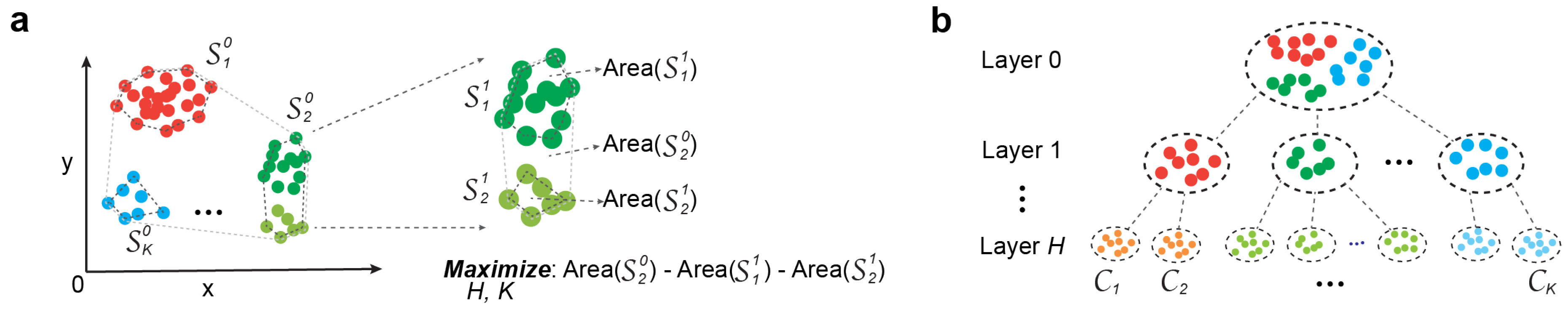
Figure 2.
The projected data in the 2D space for the dataset Biase
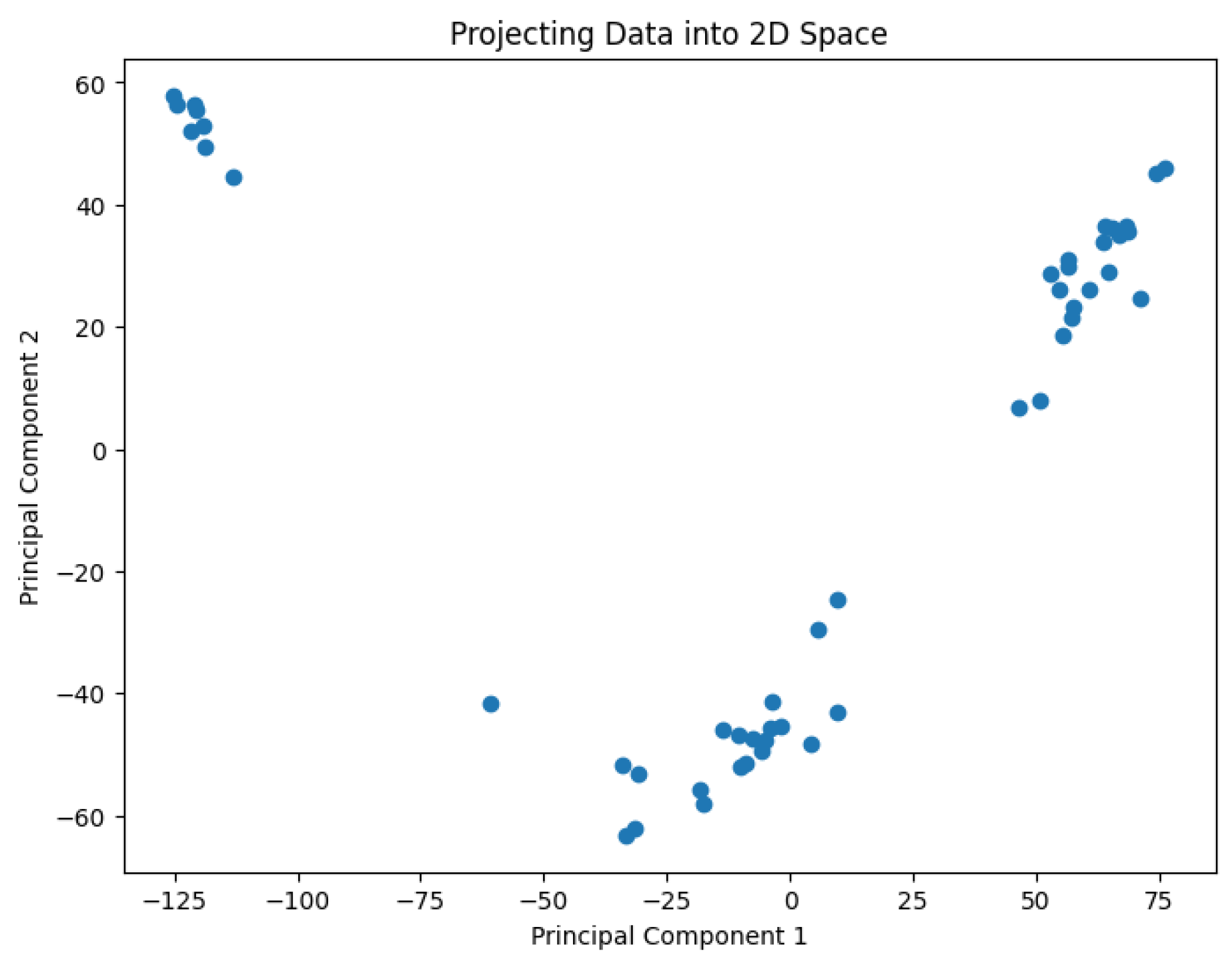
Figure 3.
The projected data in the 2D space for the dataset Deng
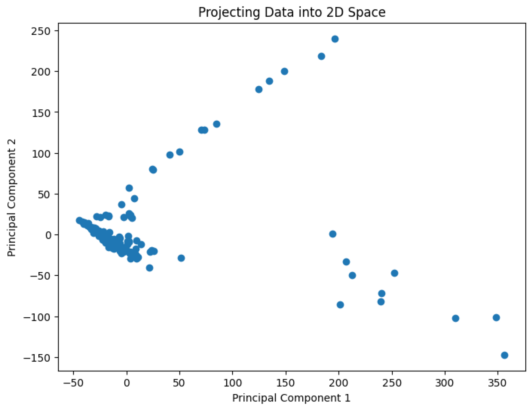
Figure 4.
The projected data in the 2D space for the dataset Goolam
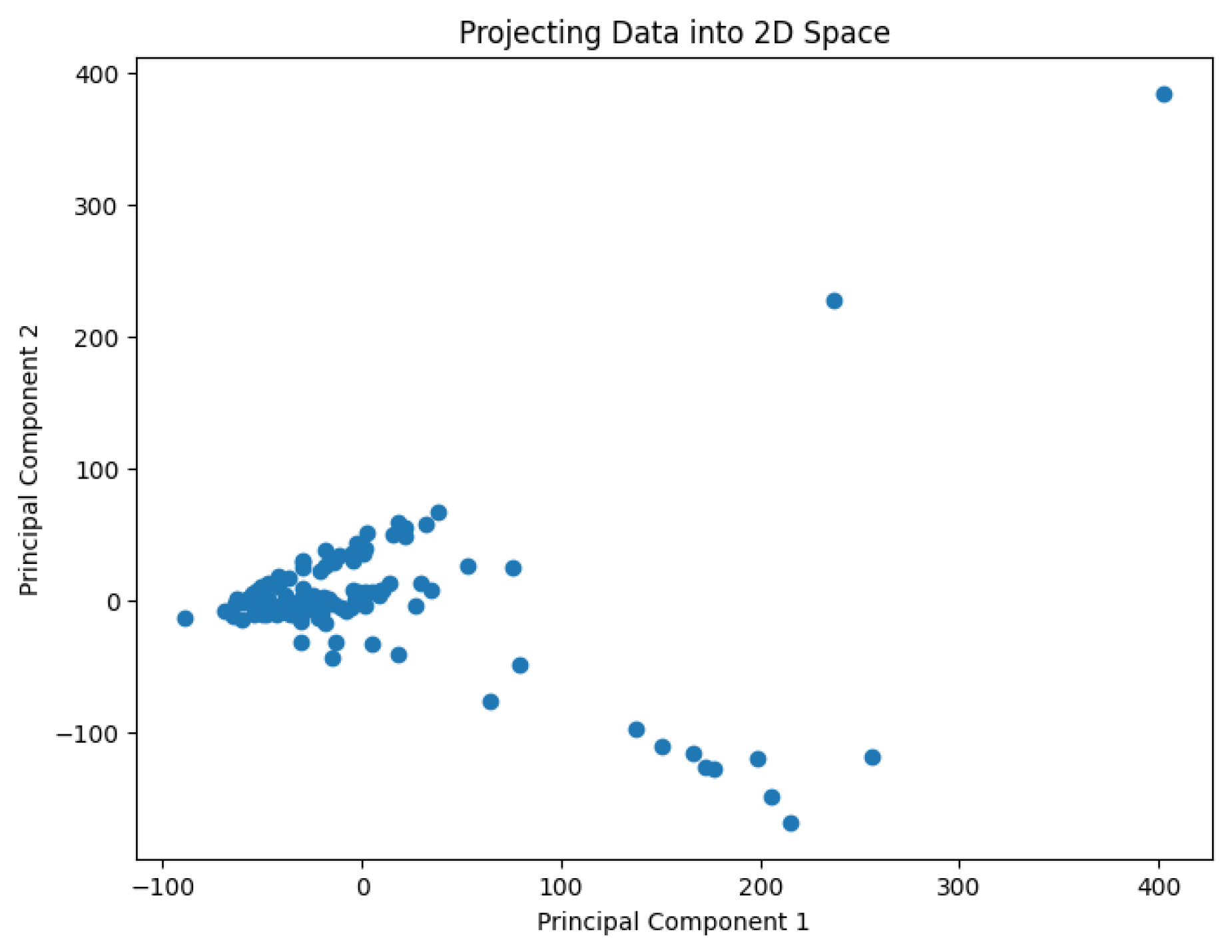
Figure 5.
The projected data in the 2D space for the dataset Ting
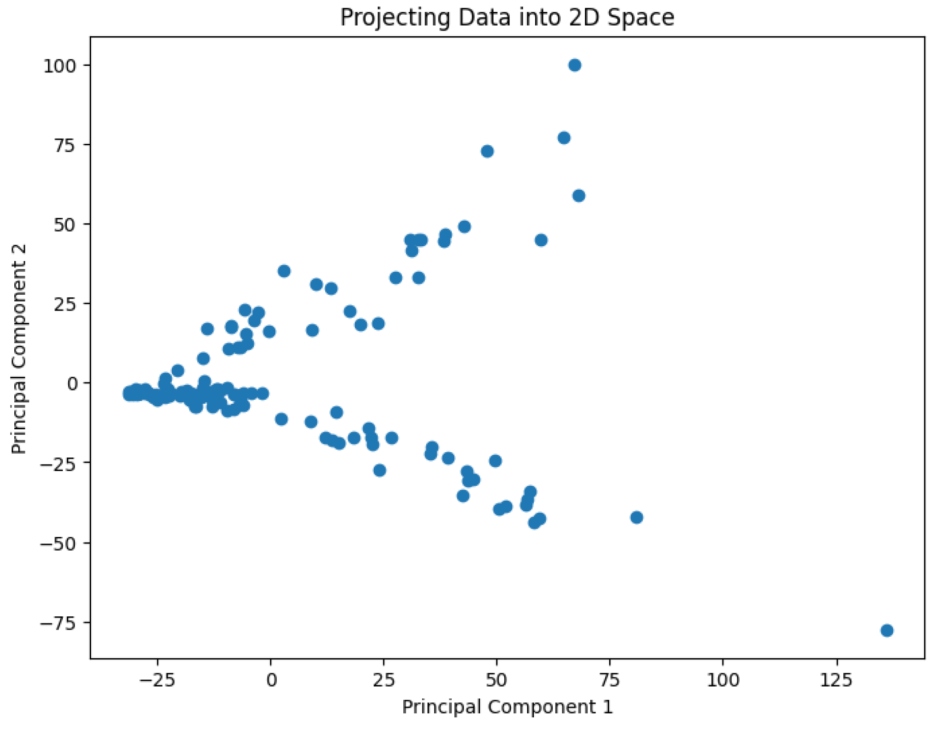
Figure 6.
The projected data in the 2D space for the dataset Yan
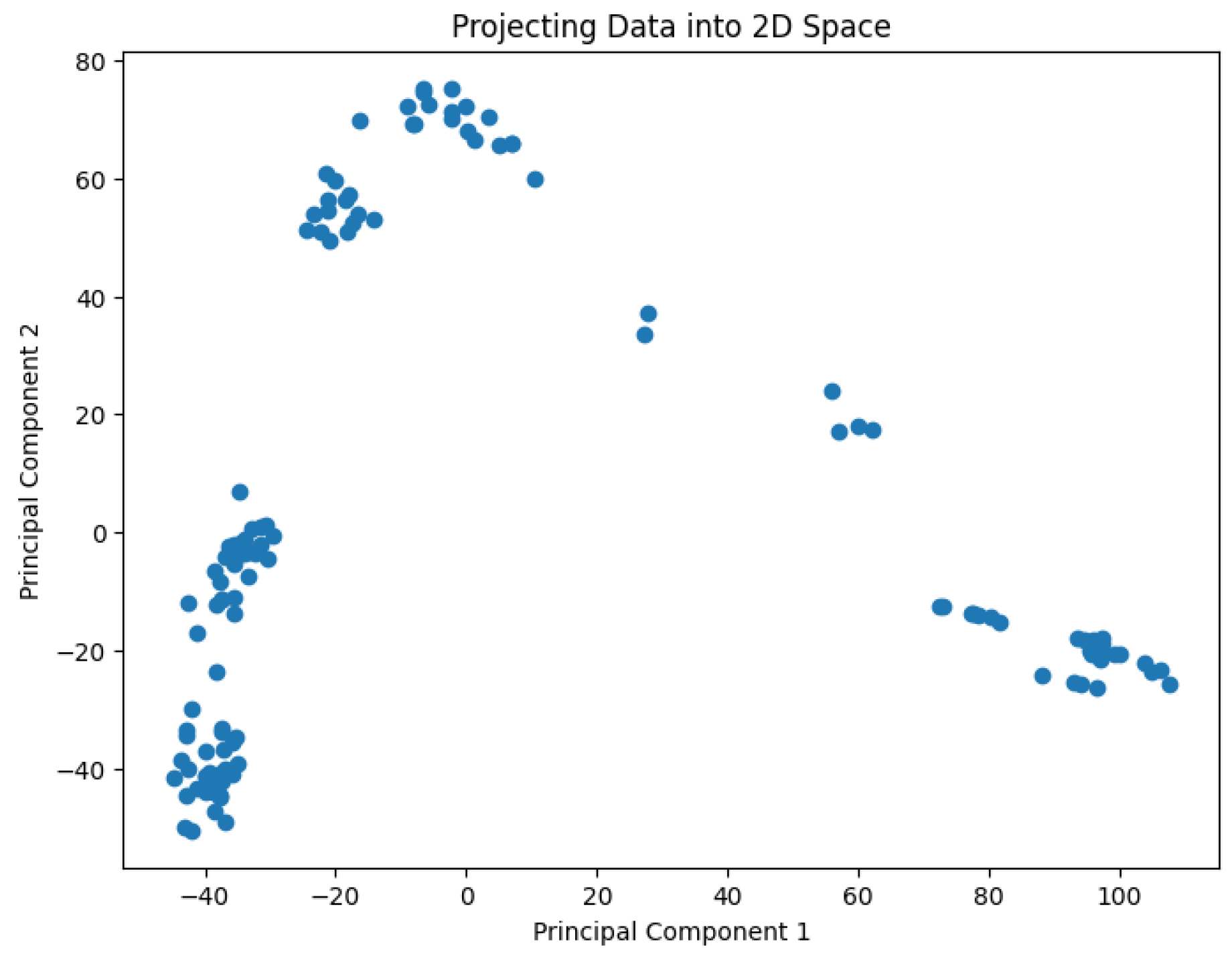
Figure 7.
The K-center clustering algorithm’s result with for the dataset Biase
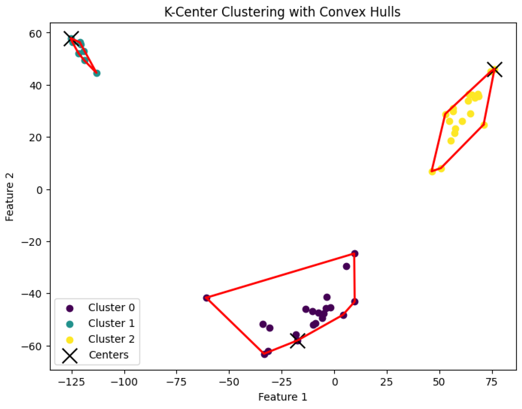
Figure 8.
The K-center clustering algorithm’s result with for the dataset Deng
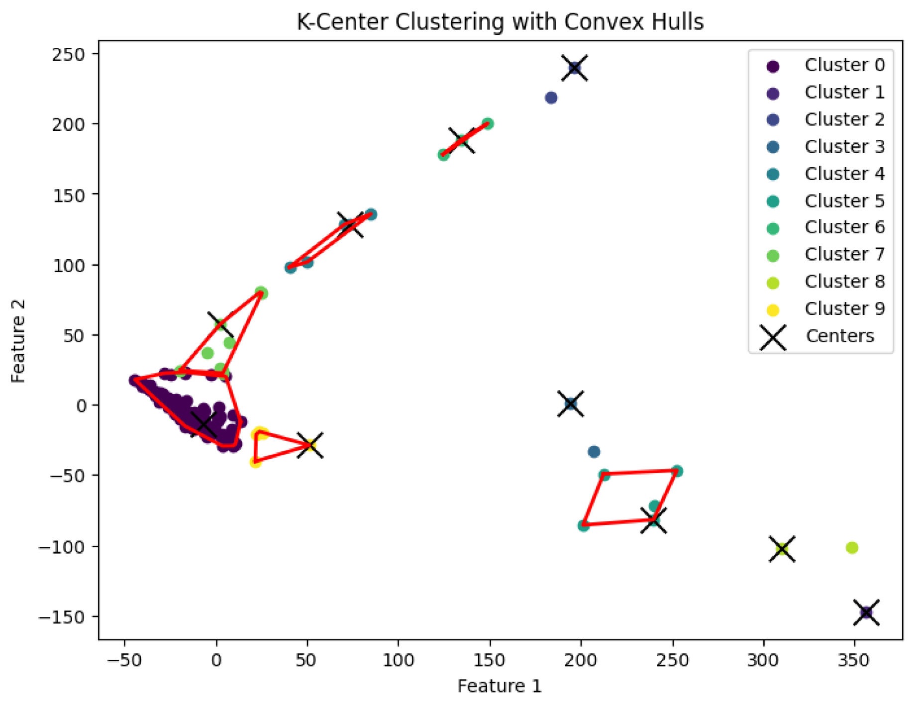
Figure 9.
The K-center clustering algorithm’s result with for the dataset Goolam
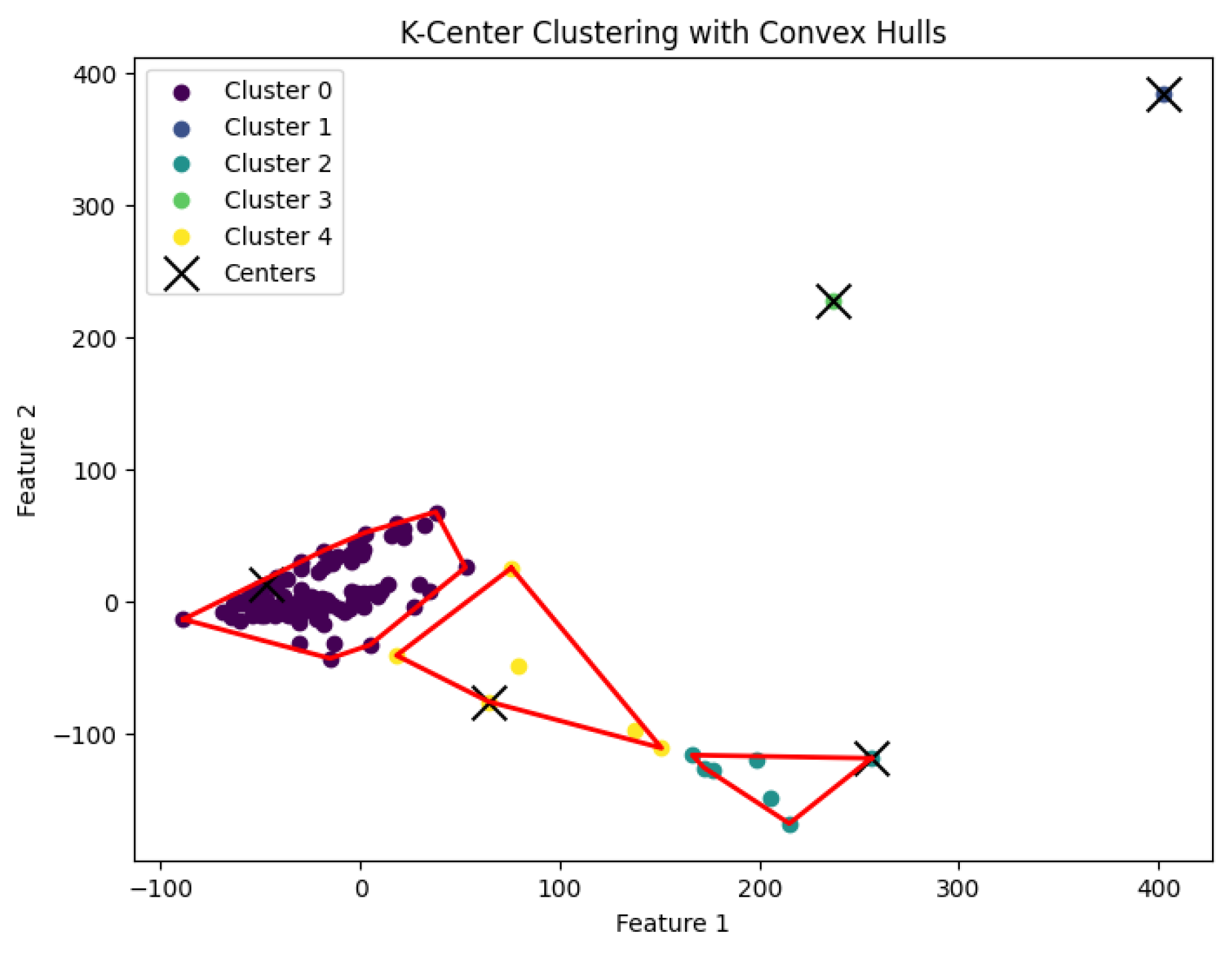
Figure 10.
The K-center clustering algorithm’s result with for the dataset Ting
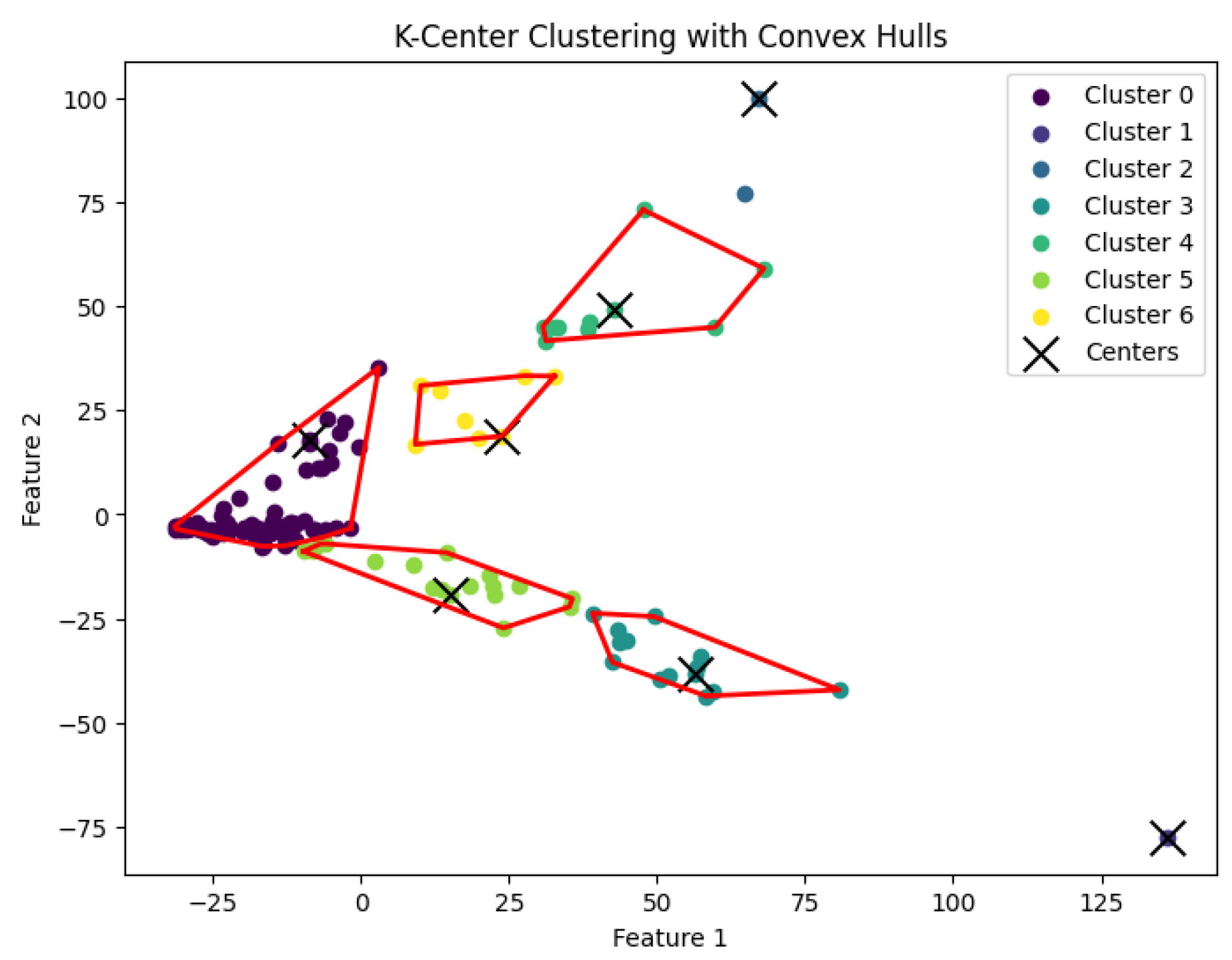
Figure 11.
The K-center clustering algorithm’s result with for the dataset Yan
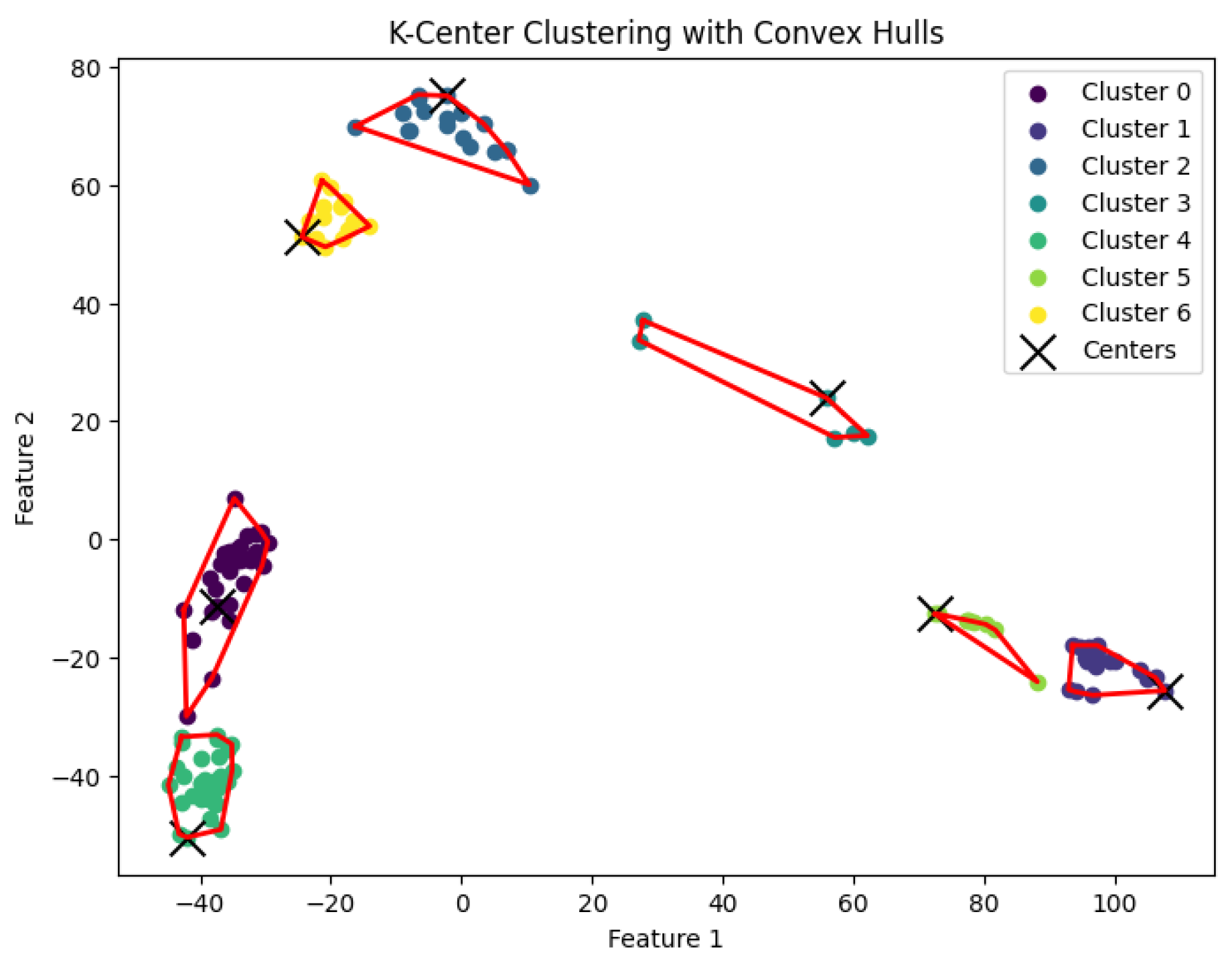
Figure 12.
The K-median clustering algorithm’s result with for the dataset Biase
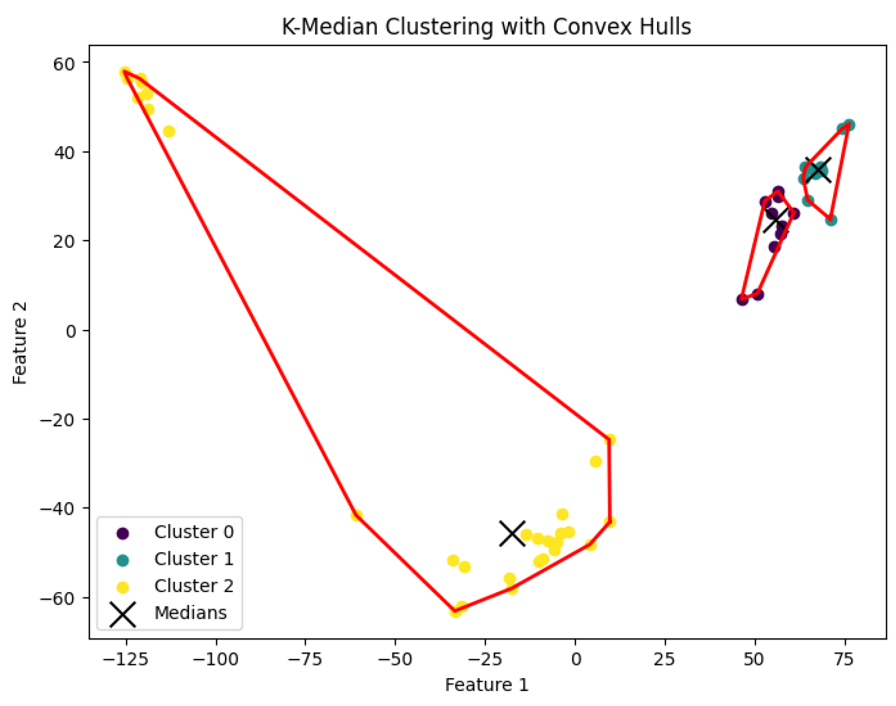
Figure 13.
The K-median clustering algorithm’s result with for the dataset Deng

Figure 14.
The K-median clustering algorithm’s result with for the dataset Goolam
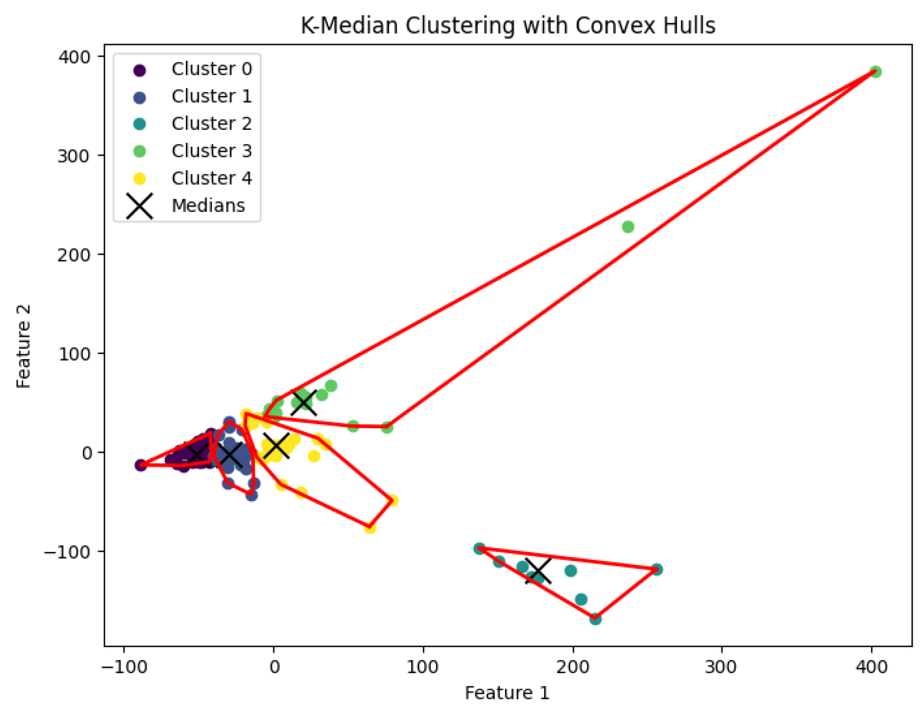
Figure 15.
The K-median clustering algorithm’s result with for the dataset Ting
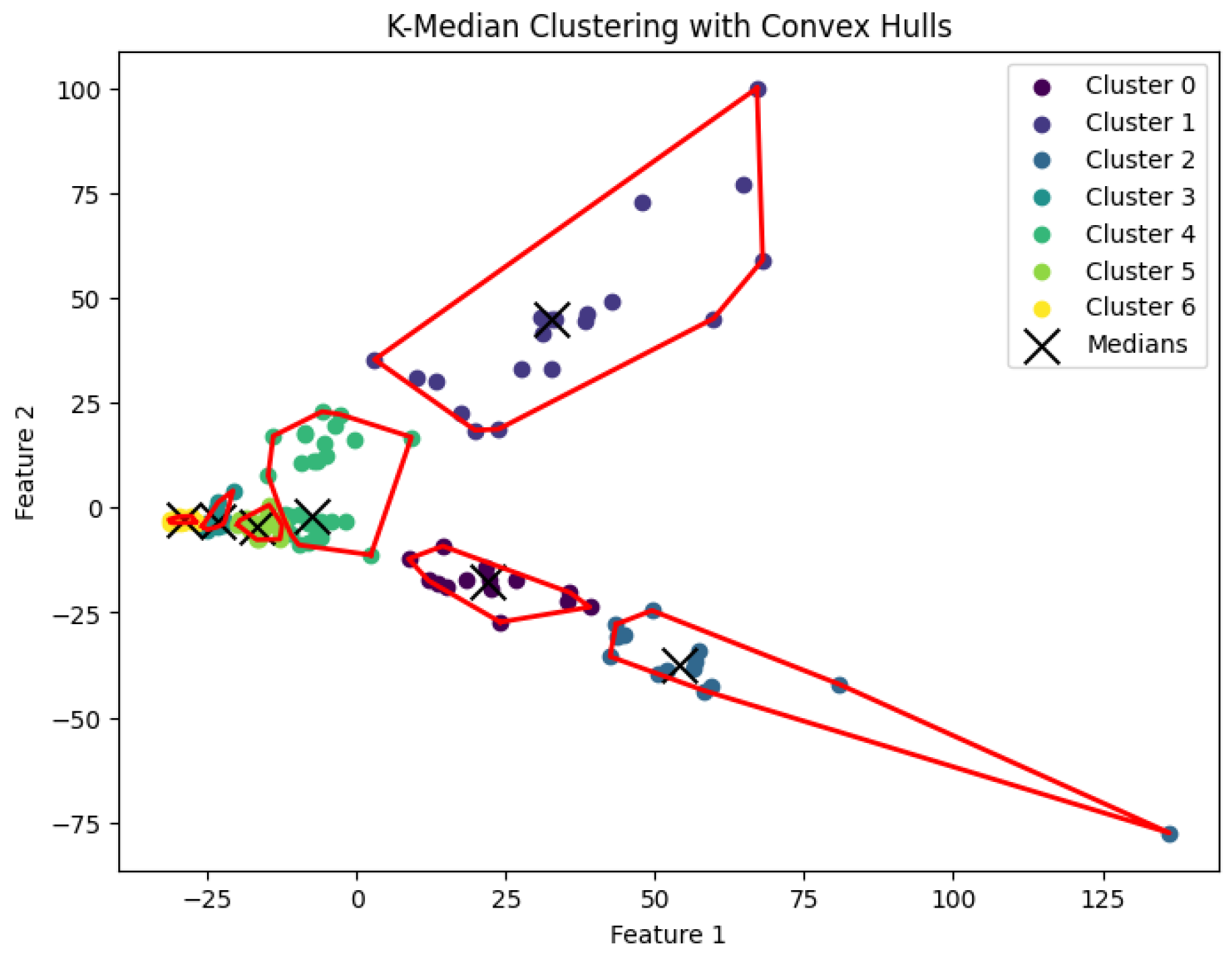
Figure 16.
The K-median clustering algorithm’s result with for the dataset Yan

Figure 17.
The K-means clustering algorithm’s result with for the dataset Biase
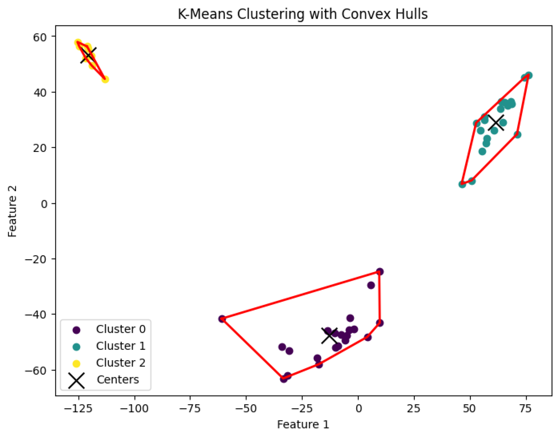
Figure 18.
The K-means clustering algorithm’s result with for the dataset Deng
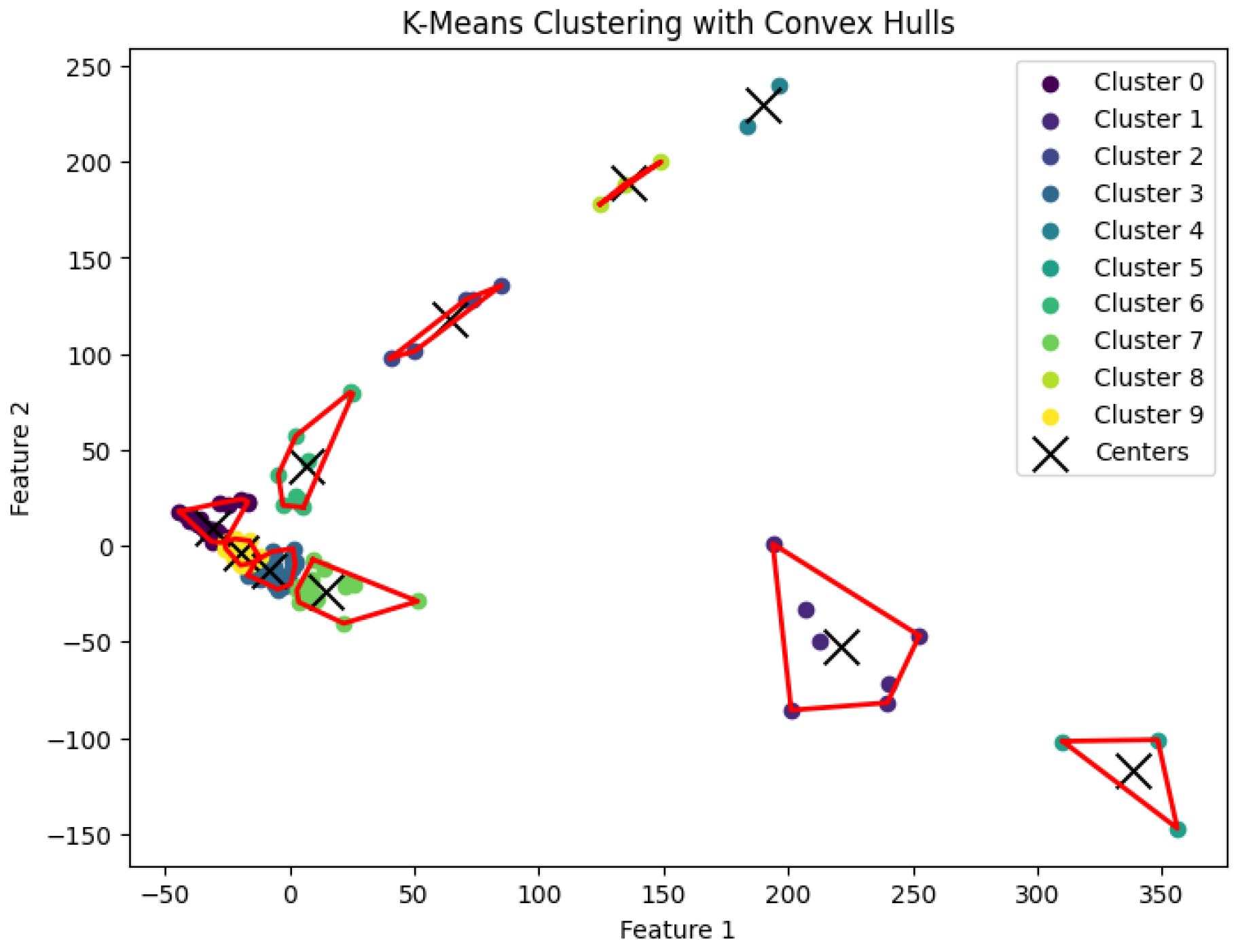
Figure 19.
The K-means clustering algorithm’s result with for the dataset Goolam
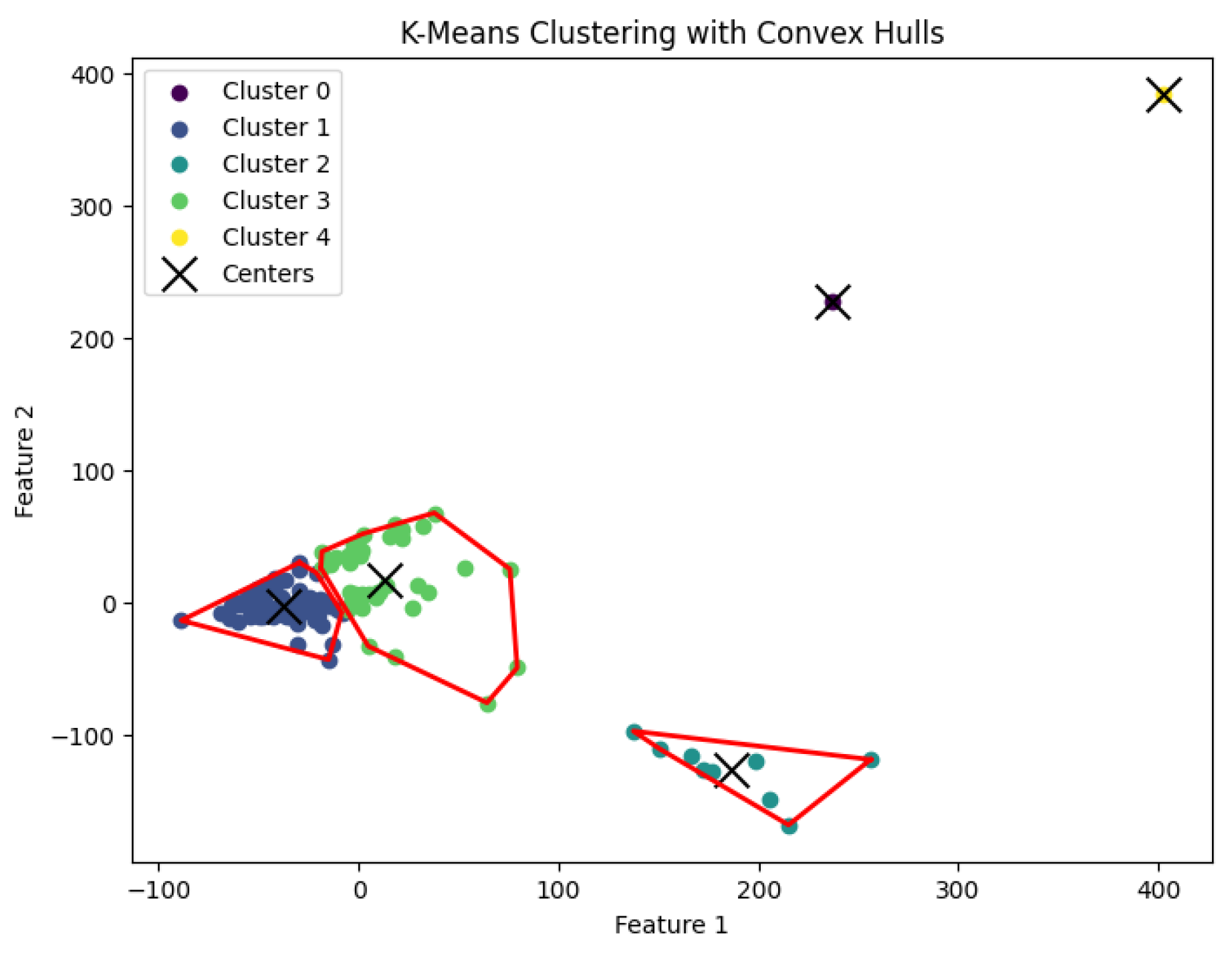
Figure 20.
The K-means clustering algorithm’s result with for the dataset Ting
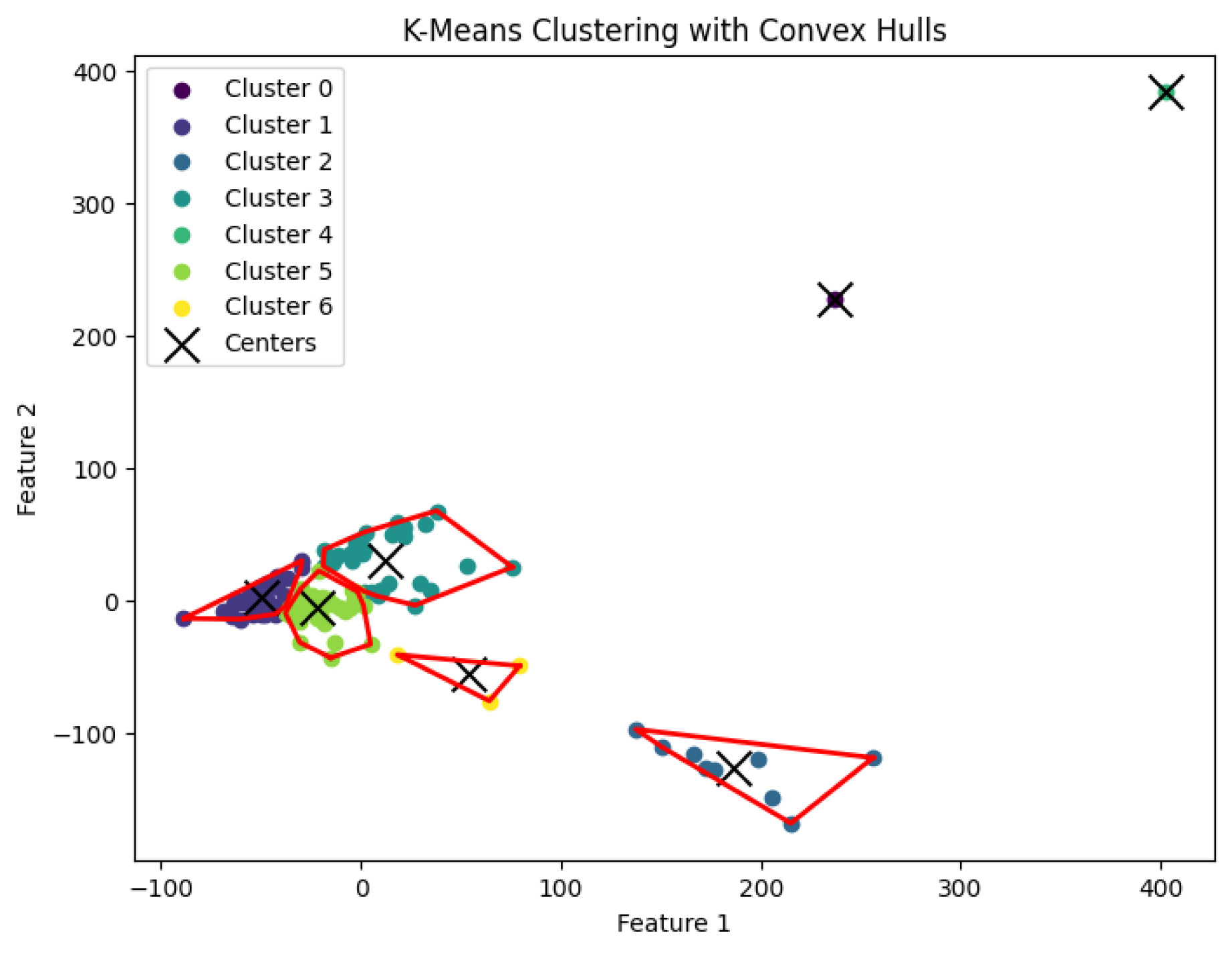
Figure 21.
The K-means clustering algorithm’s result with for the dataset Yan
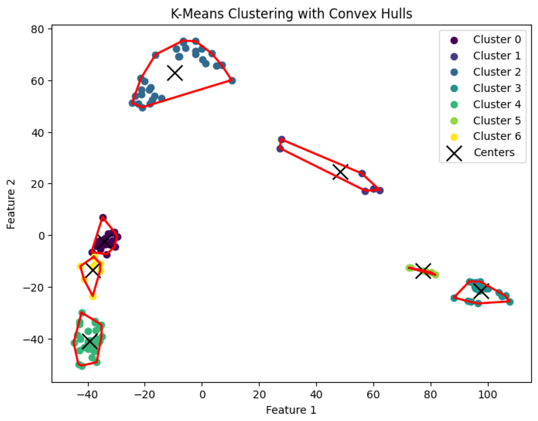
Figure 22.
The K-area clustering algorithm’s result with for the dataset Biase
Figure 23.
The K-area clustering algorithm’s result with for the dataset Deng
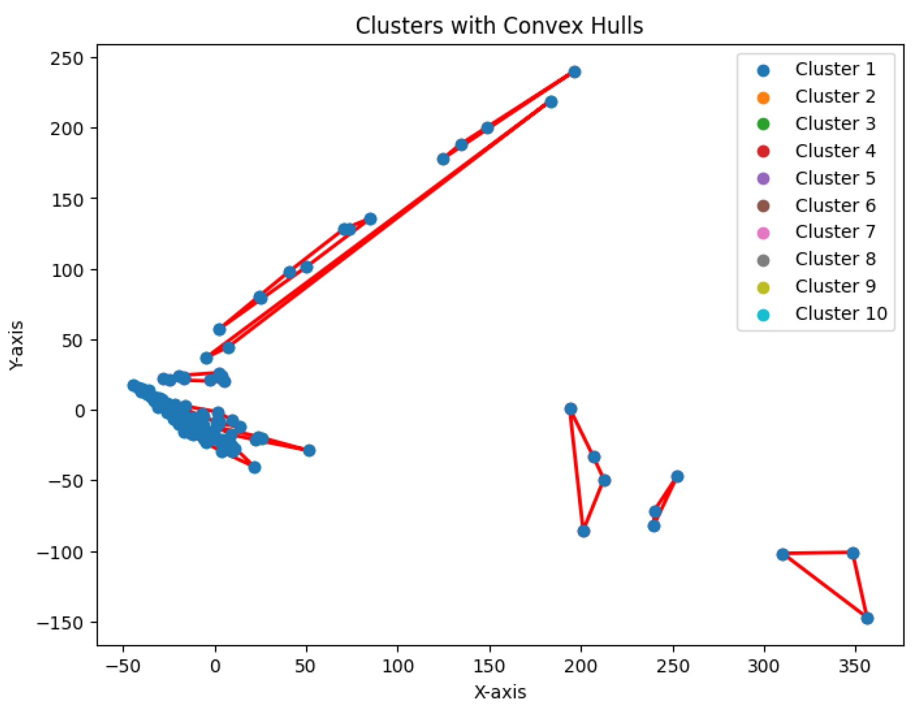
Figure 24.
The K-area clustering algorithm’s result with for the dataset Goolam
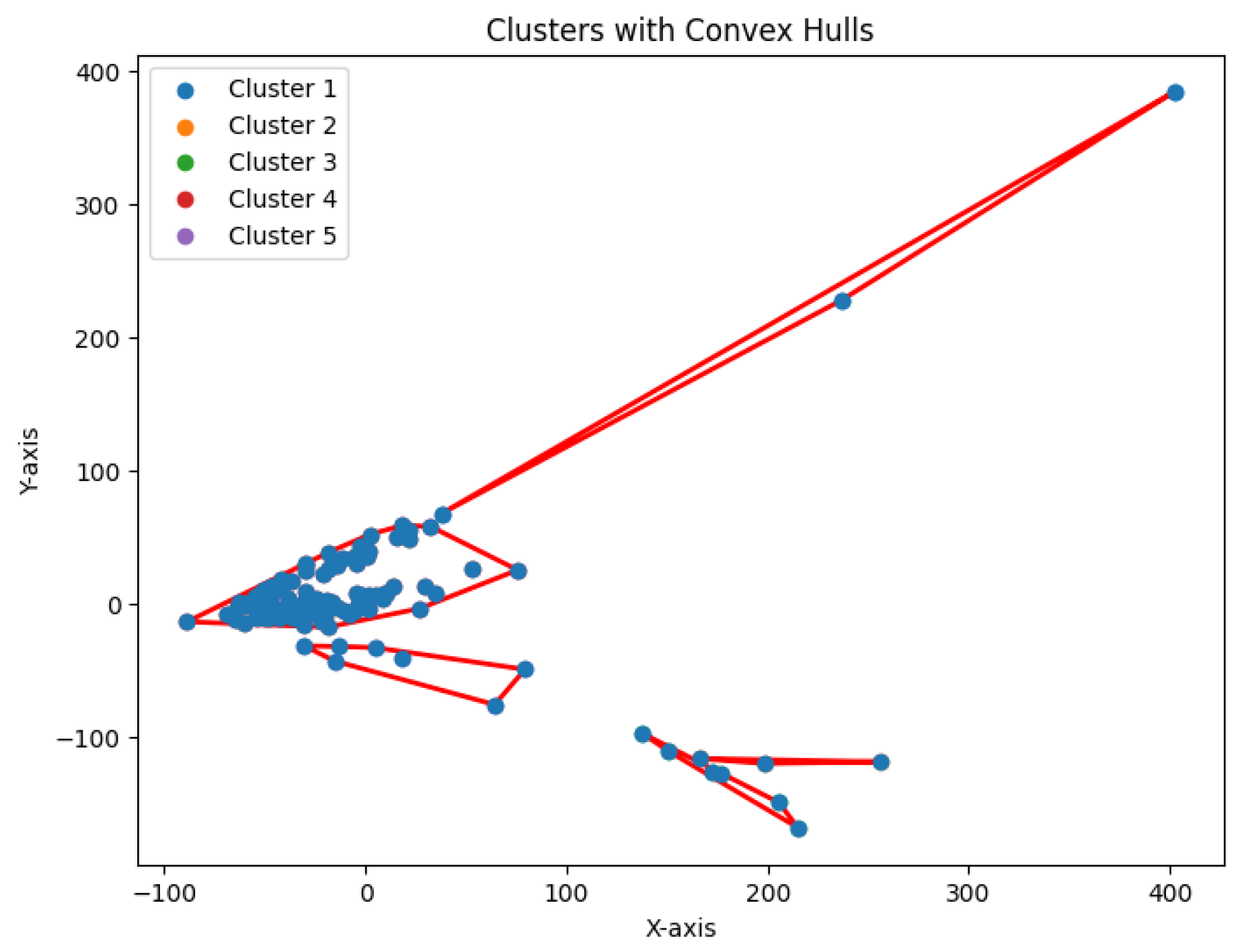
Figure 25.
The K-area clustering algorithm’s result with for the dataset Ting

Figure 26.
The K-area clustering algorithm’s result with for the dataset Yan
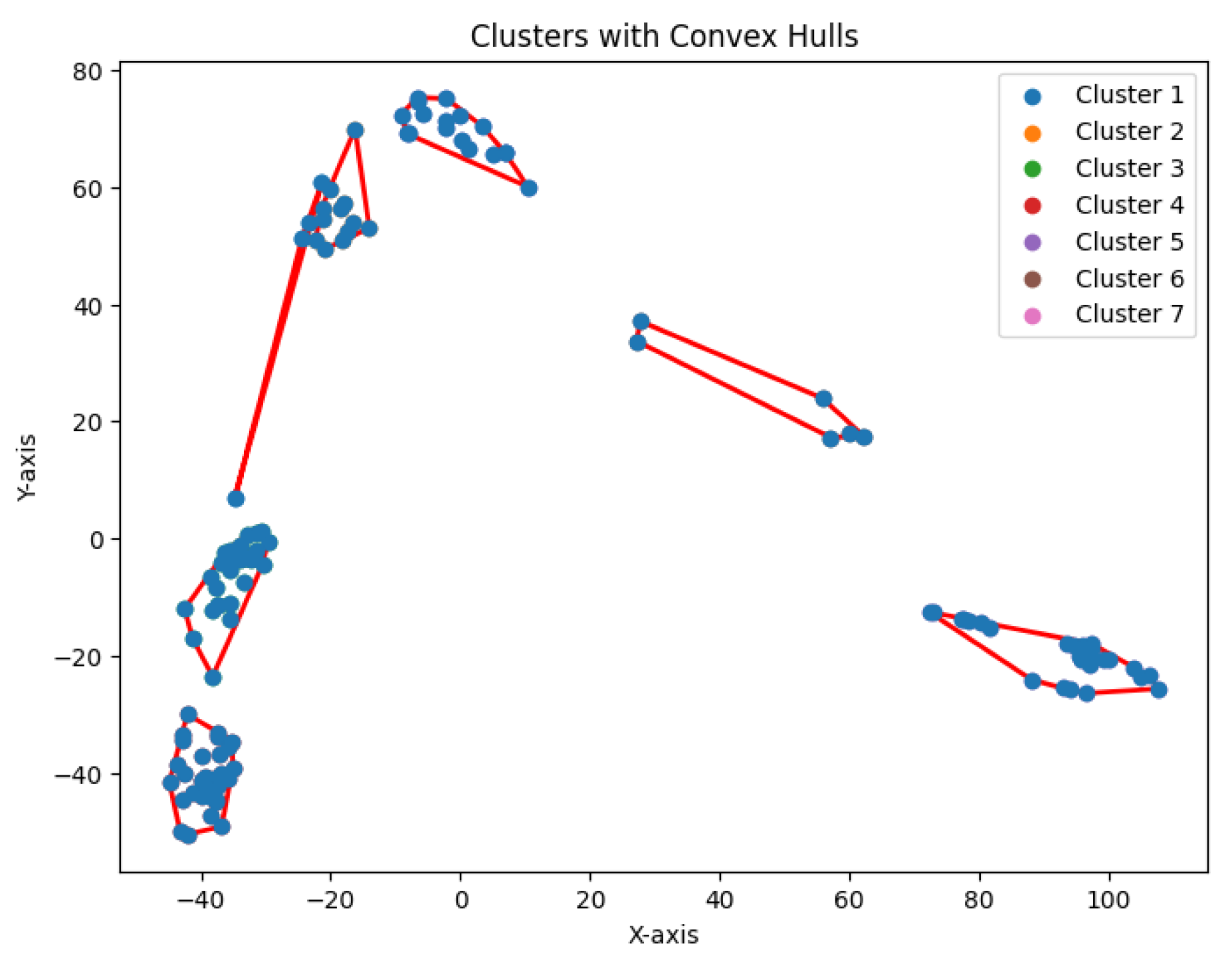
Figure 27.
Comparison of four clustering algorithms based on their performance, evaluated using NMI values.
Figure 27.
Comparison of four clustering algorithms based on their performance, evaluated using NMI values.
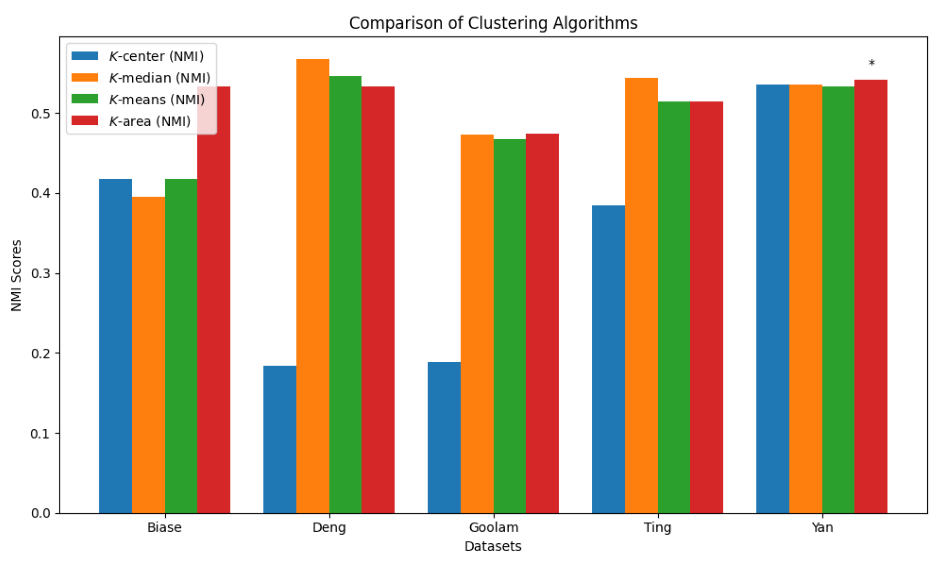
Figure 28.
Comparison of four clustering algorithms based on their performance, evaluated using convex area sizes
Figure 28.
Comparison of four clustering algorithms based on their performance, evaluated using convex area sizes
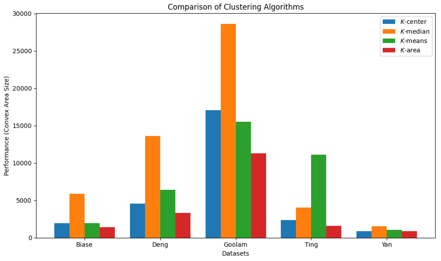
Figure 29.
The area ratios reveal the number of clusters needed
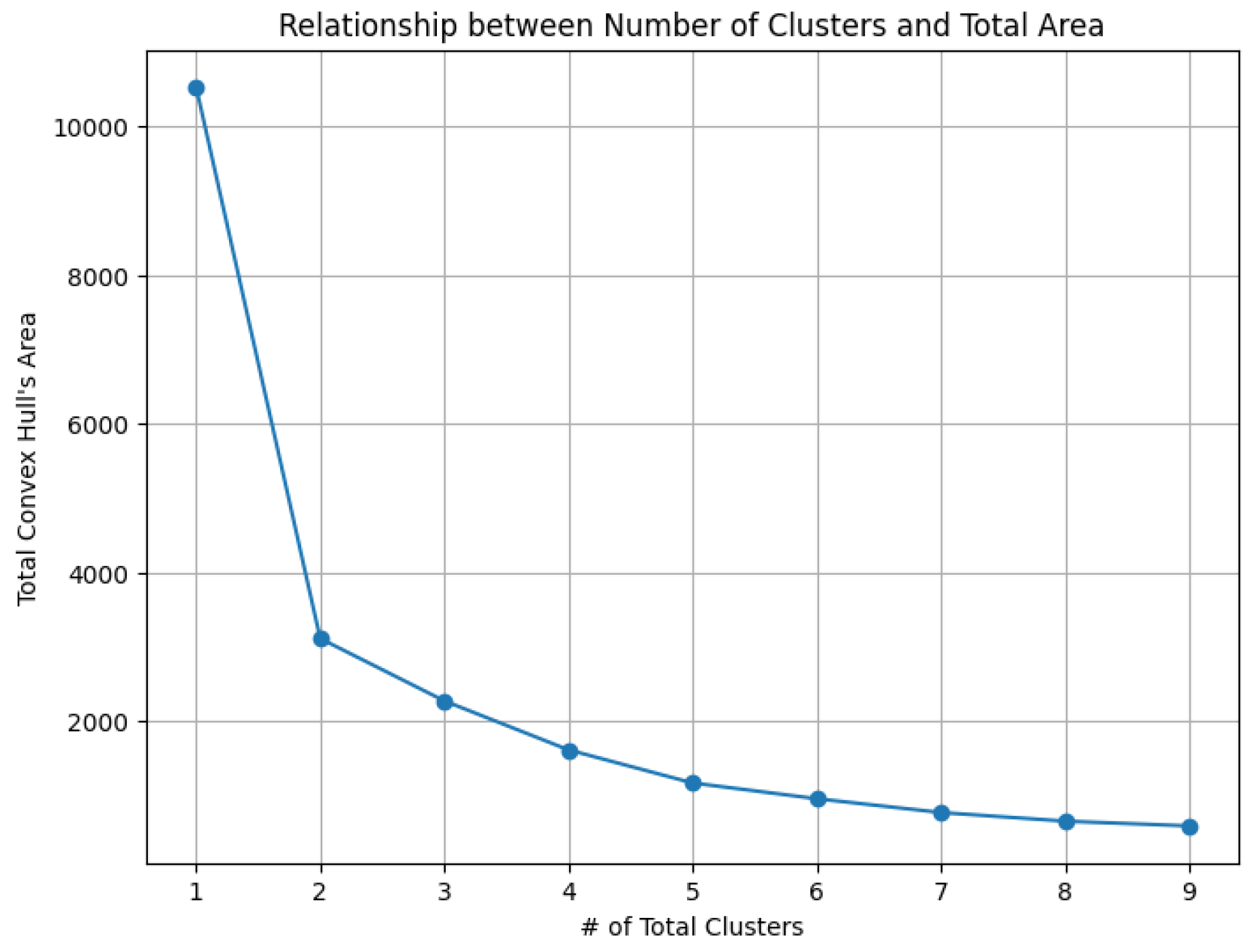
Figure 30.
One cluster for Yan
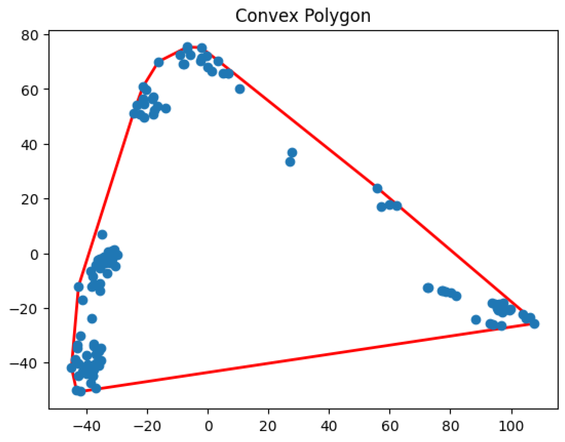
Figure 31.
Two clusters for Yan
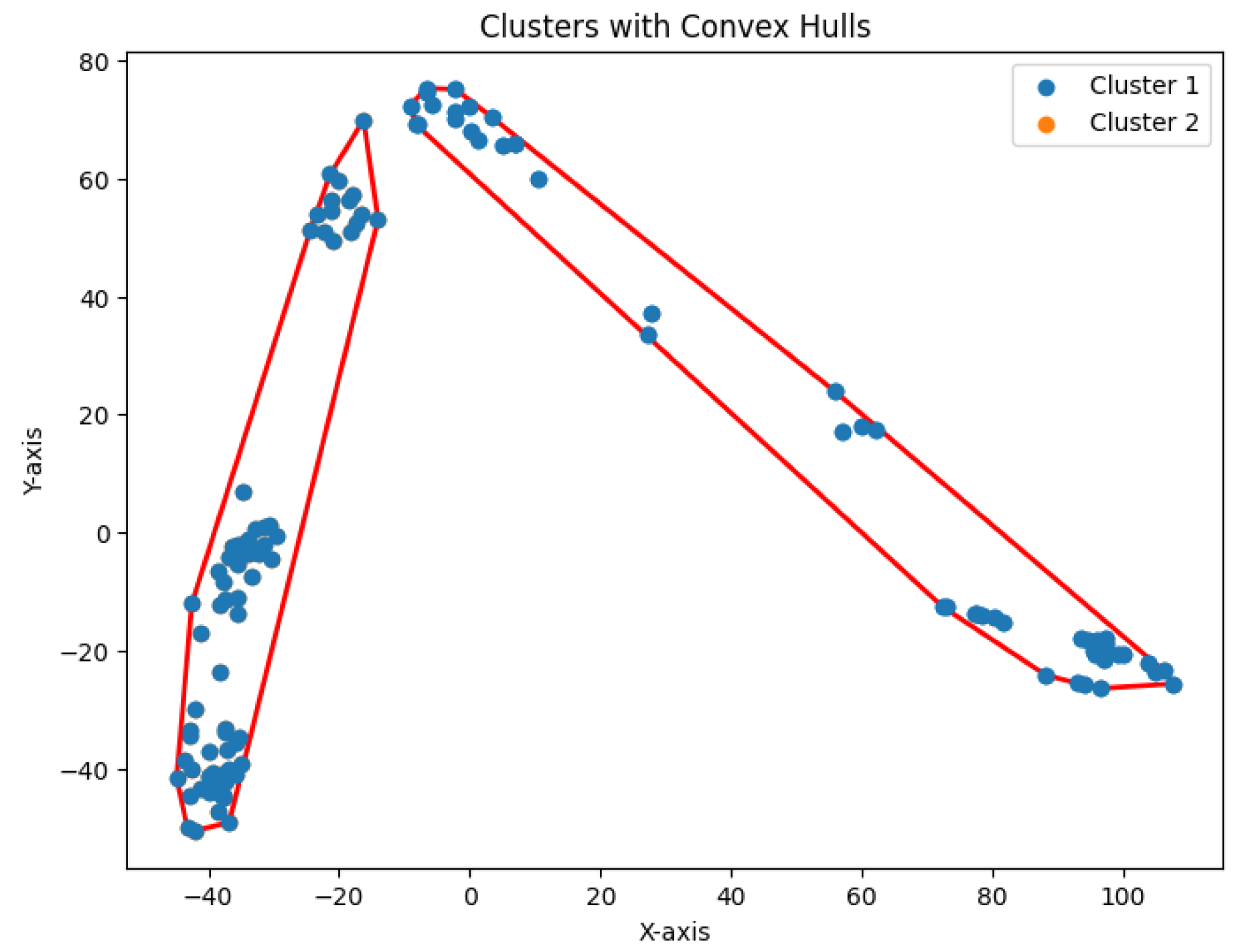
Figure 32.
Three clusters for Yan
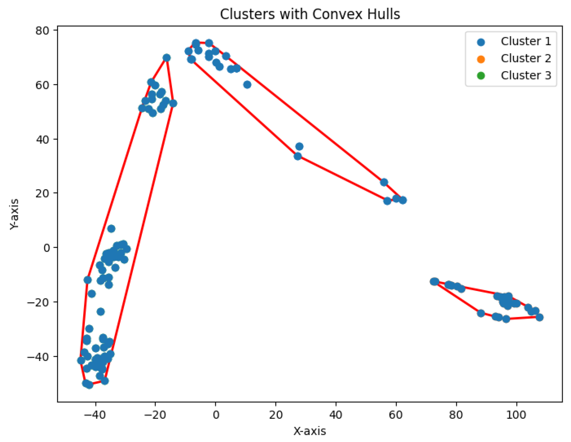
Figure 33.
Four clusters for Yan
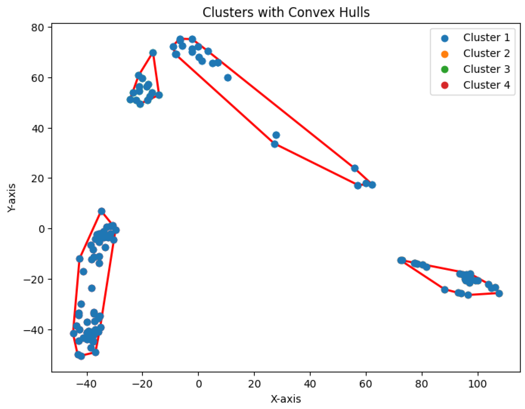
Figure 34.
Five clusters for Yan
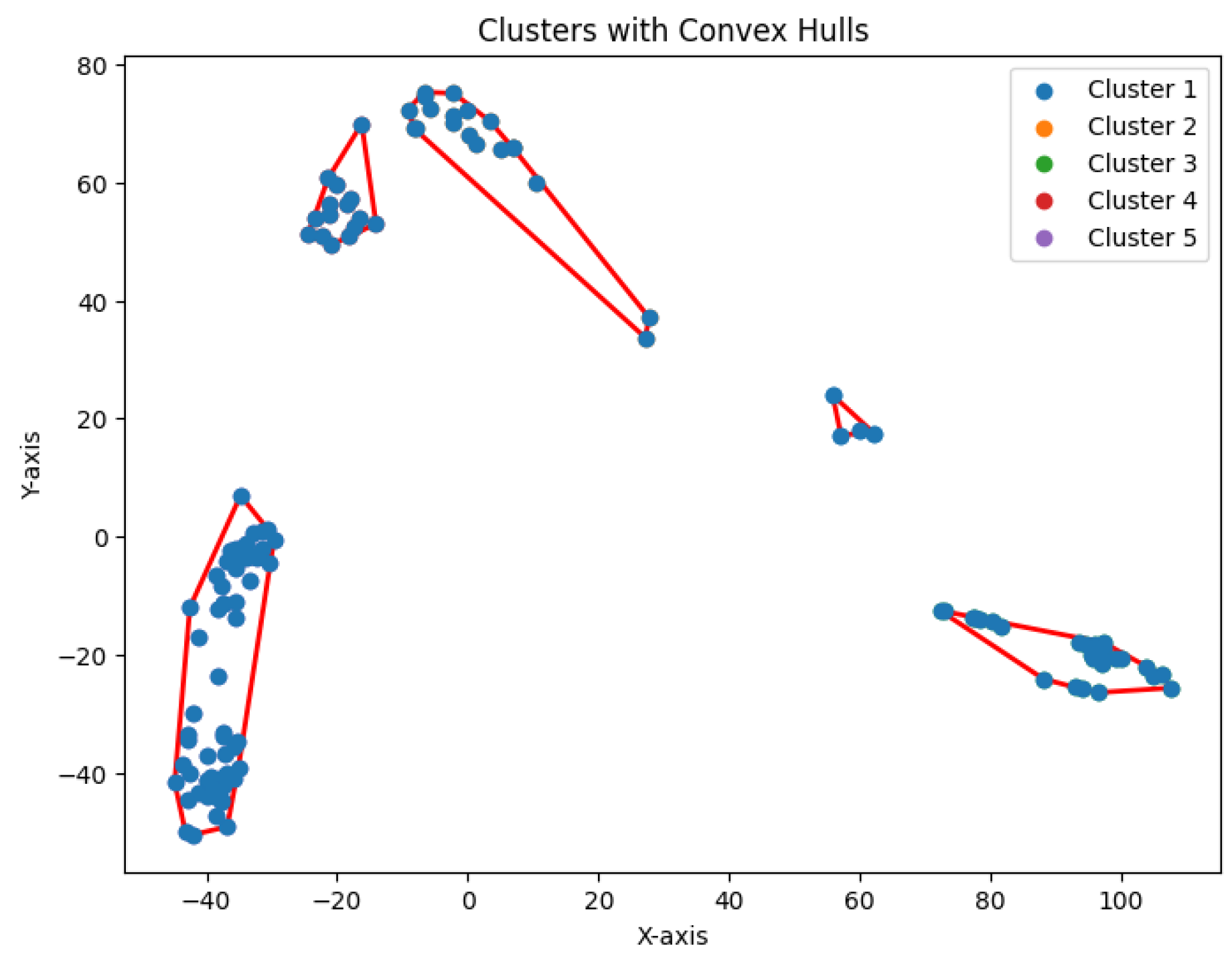
Figure 35.
Six clusters for Yan
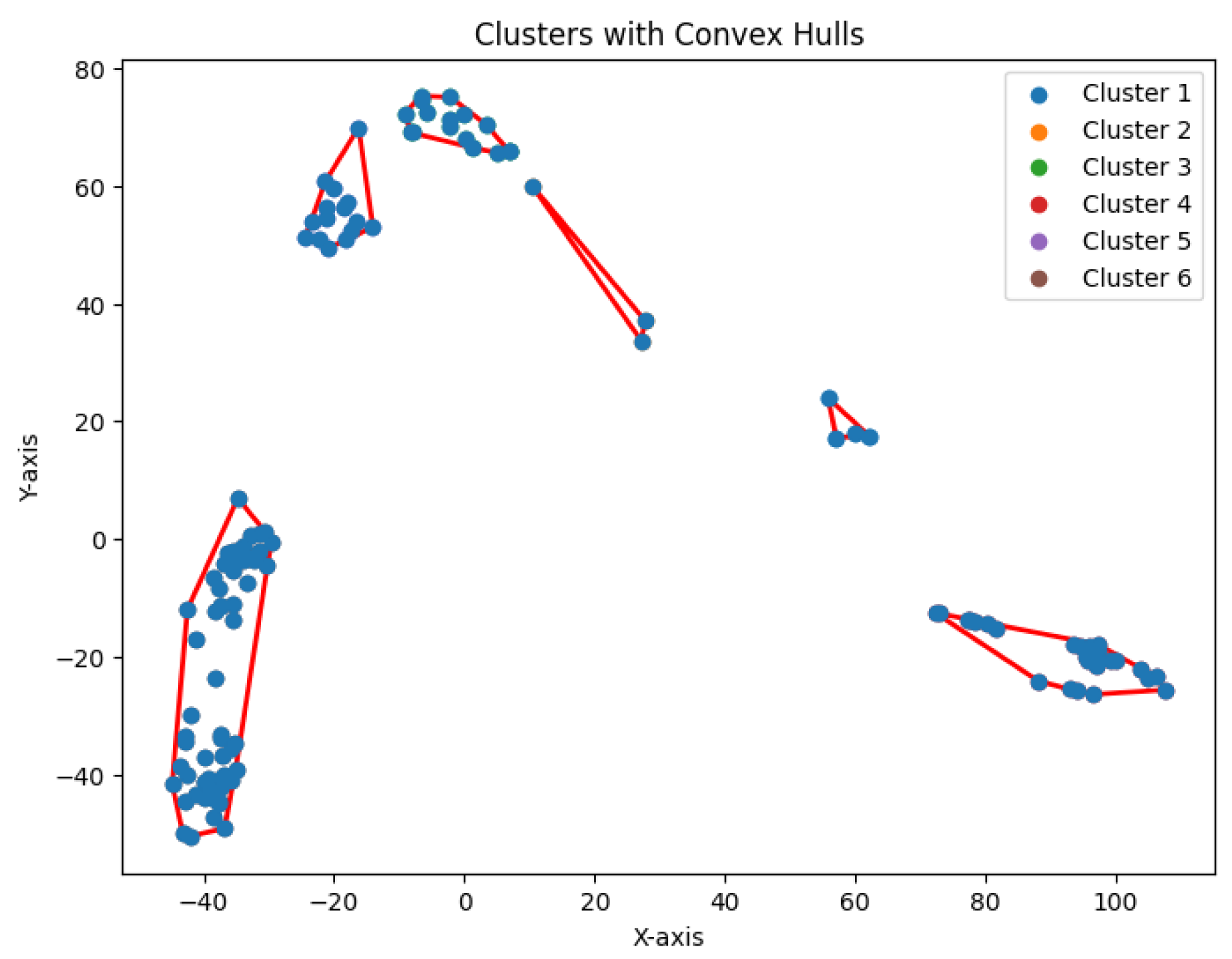
Figure 36.
Seven clusters for Yan
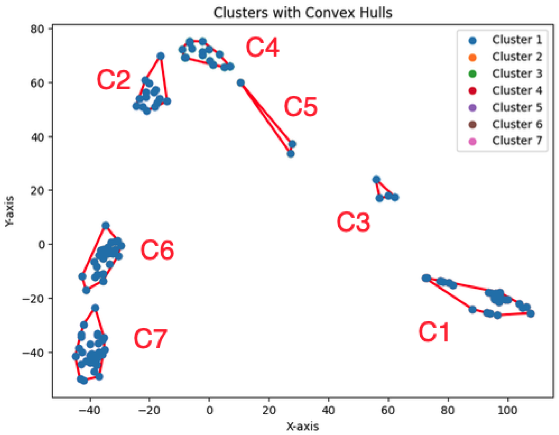
Figure 37.
The tree structure representing the partition made by the K-area algorithm
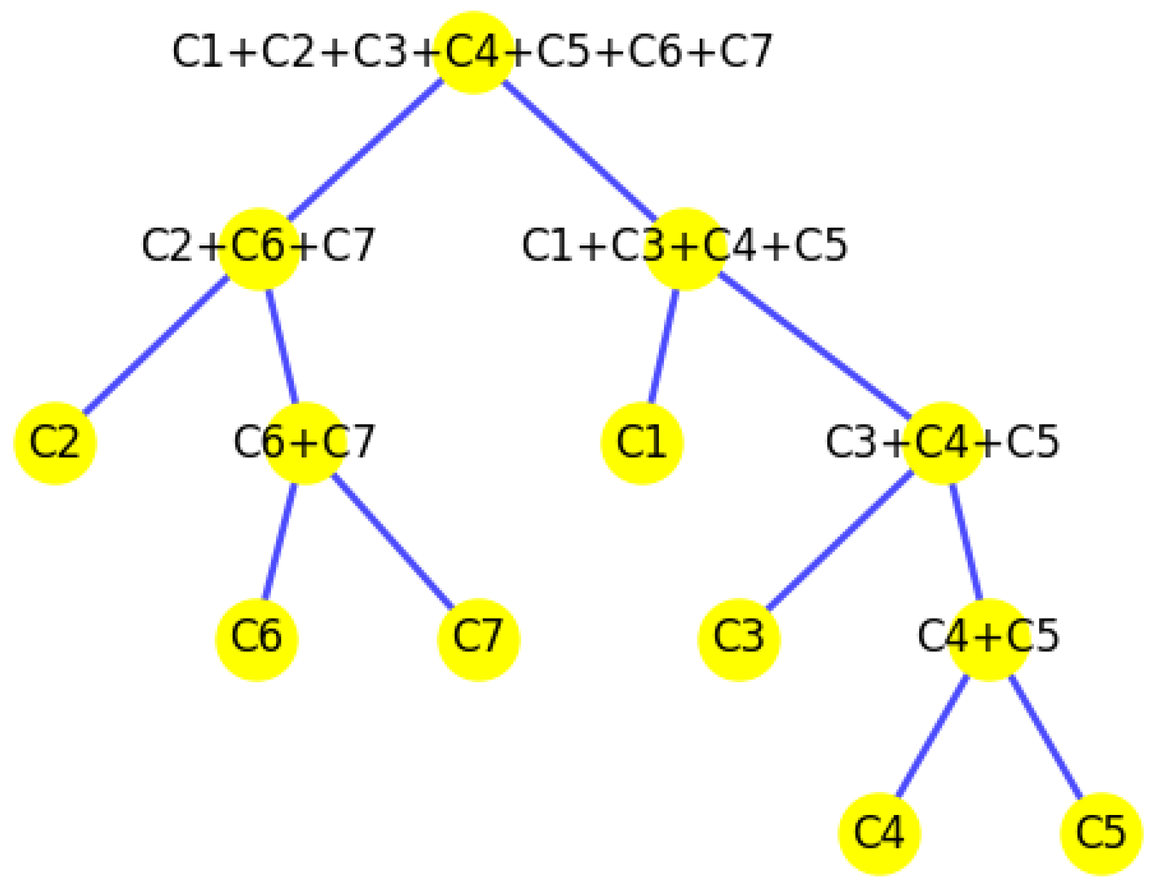
Table 1.
Types of clustering algorithms. *: denotes our approach in this paper.
| Center-based clusters | High-density clusters | Center-based density clusters* | ||
| K-center clustering | K-median clustering | K-means clustering | K-high-density regions | K-volume clustering* |
| NP-hard | NP-hard | NP-hard | NP-hard | - |
| An iterative greedy algorithm [4] | An iterative greedy algorithm [5] | An iterative greedy algorithm [23] | An iterative greedy algorithm [24] | An iterative greedy algorithm* |
Table 3.
Comparison of four clustering algorithms based on their performance, evaluated using NMI values. We use * to denote the best results.
Table 3.
Comparison of four clustering algorithms based on their performance, evaluated using NMI values. We use * to denote the best results.
| Dataset \ Algorithms | K-center | K-median | K-means | K-area |
| Biase | ||||
| Deng | ||||
| Goolam | ||||
| Ting | ||||
| Yan |
Table 4.
Comparison of four clustering algorithms based on their performance, evaluated using convex area sizes
Table 4.
Comparison of four clustering algorithms based on their performance, evaluated using convex area sizes
| Dataset Algorithms | K-center | K-median | K-means | K-area |
| Biase | ||||
| Deng | ||||
| Goolam | ||||
| Ting | ||||
| Yan |
Table 5.
The total clusters’ area and the ratios of the convex hull areas between two neighboring rounds help determine the value K
Table 5.
The total clusters’ area and the ratios of the convex hull areas between two neighboring rounds help determine the value K
| # of total cluster | Total convex hull’s area | Area ratios of two neighboring rounds |
| 1 | 10530.41 | 0 |
| 2 | 3110.62 | 0.30 |
| 3 | 2271.75 | 0.73 |
| 4 | 1613.22 | 0.71 |
| 5 | 1167.92 | 0.72 |
| 6 | 956.11 | 0.82 |
| 7 | 770.70 | 0.81 |
| 8 | 654.54 | 0.85 |
| 9 | 590.55 | 0.90 |
Disclaimer/Publisher’s Note: The statements, opinions and data contained in all publications are solely those of the individual author(s) and contributor(s) and not of MDPI and/or the editor(s). MDPI and/or the editor(s) disclaim responsibility for any injury to people or property resulting from any ideas, methods, instructions or products referred to in the content. |
© 2025 by the authors. Licensee MDPI, Basel, Switzerland. This article is an open access article distributed under the terms and conditions of the Creative Commons Attribution (CC BY) license (http://creativecommons.org/licenses/by/4.0/).
Copyright: This open access article is published under a Creative Commons CC BY 4.0 license, which permit the free download, distribution, and reuse, provided that the author and preprint are cited in any reuse.


