
Submitted:
05 February 2025
Posted:
05 February 2025
You are already at the latest version
Abstract
This paper presents efficient coupling methods that accurately reduce the computational cost for modelling solids dynamically with finite elements. A multi-time step integration algorithm is developed to leverage varying time steps throughout a domain. Interfaces between subdomains are resolved explicitly with the continuity of acceleration and tractions. A spatial coupling method is combined with multiple time steps, allowing for meshes that do not necessarily conform at their interfaces. The method avoids solving additional degrees of freedom at these interfaces, with parameter-free coupling operators defined between meshes. A speedup >12X is achieved in comparison to reference single time step methods.
Keywords:
Multi-Time Stepping
; Non-Matching Meshes
; Explicit Finite Elements
1. Introduction
The temporal and spatial discretisation of structural dynamic problems is directly related to the accuracy and computational cost of the explicit finite element method. Constrained by the Courant-Friedrichs-Lewy (CFL) condition, the critical time step, is proportional to the element size, and inversely to the dilatational wave speed [1]. This leads to simulations being restricted to of the element with the smallest size or highest wave speed. Initially referred to as subcycling, pioneering works allowed for the integration of multiple time steps in a single domain [2,3]. The coupling of various kinematic fields was explored, along with the stability of such algorithms [4,5]. Asynchronous variational integration is briefly mentioned as an alternative; that discretise the functional instead of the equations of motion, with varying time steps [6]. The main drawback being the high complexity of its implementation. The importance of varying, non-integer and large time step ratios was also extended to, with heterogeneous asynchronous time integration [7,8]. However, maintaining the continuity of kinematics at the interface remains a challenge, especially for all three fields [9]. In recent works, energy conserving methods have been developed, however they depart far from the CFL condition to resolve the interface conditions at consistent time steps [10]. Spatially, non-matching mesh algorithms facilitate more flexible geometric modelling [11]. Nitsche’s method has shown to weakly enforce conditions on the interfaces of non-matching meshes without additional unknowns, but commonly suffers from the sensitivity to parameters [12,13,14,15]. Following similar principles of weak continuity, Lagrange multipliers are called upon in the mortar-based methods [16,17,18,19,20]. These types of methods have proven to be very robust, however struggle to fulfil the inf-sup stability condition, and incur a large computational cost with mapping master and slave nodes [21]. In comparison, the use of localised Lagrange multipliers, introduces a frame that independently enforces compatibility constraints on each boundary [22,23,24,25,26,27]. However, as common with other methods that introduce an additional discretised interface, the construction of this interface is neither trivial or computationally cheap [28,29,30,31]. This brief review justifies the need for more efficient couplings; both temporally and spatially. Coupling algorithms that allow for varying time step ratios, whilst stepping close to the CFL condition, concertedly those that solve for non-matching meshes, without increasing the degrees of freedom, remain a hot topic of research.
2. Governing Equations of Dynamic Solids
The problem of a solid body subject to impact, is described through the partitioning of a domain as illustrated in Figure 1. The deformation is governed by the momentum balance equation acting on solid domain :
where , , and denote the density, acceleration field, stress tensor and body forces. Deformation is described at time for a specified constant . Updated Lagrangian formulations of a single body are found in the following [32,33,34], here we extend this to a partitioned formulation to solve multiple solid subdomains.
Defining multiple subdomains, we state is a solid body in an open region , with its boundary denoted . is partitioned into non-overlapping subdomains:
Starting from the simplest case, , for a two-subdomain partitioning, where and represent the large and small subdomains. The boundary between the two is defined , where for matching conditions we enforce:
to ensure the continuity of acceleration and tractions , as well as enforcing Dirichlet and Neumann boundary conditions. The variational formulation of the dynamic equilibrium in Equation 1 can be described for both and as the following:
where we denote a variational velocity , in a space where , and as rate of deformation. A discrete approximation of the variational form can be reduced to the ordinary differential equations:
where for subdomains and , we sum over a number of finite elements, and , in each subdomain:
The Lagrangian shape functions are represented by , with their derivatives denoted . As common within the explicit finite element method, is lumped for each subdomain, with and both computed with vectors too. We elect to use the leapfrog time integration scheme to step through time, staggering the solution of each kinematic quantity such that:
noting that a diagonal mass matrix allows for a direct computation of acceleration. Velocity is computed on the half time step, with displacement found each full time step. Next we summarise the temporal coupling, enabled by multi-time step (MTS) integration.
3. Multi-Time Step Integration
Multi-time stepping enables partitioned subdomains and to integrate with and , respectively. However, to allow for this difference in time steps, special attention must be given to the solution of the interface . Crucially, the conditional stability of explicit methods require an element’s time step to obey the CFL condition for a linear undamped system:
Here we represent as the critical time step, as the maximum eigenfrequency, as the characteristic length of an element, and the dilatational (longitudinal) wave speed.
3.1. Salient Multi-Time Stepping Features
The asynchronous integration is enabled with three important groups of computations. The first being the explicit computation of the acceleration on the interface :
We define indicator matrices (vectors in 1-D) for each subdomain to identify the degrees of freedom on the interface of subdomains. These summations provide the ingredients for computing the interface acceleration as:
where we compute at each large time step . The integration of the subdomains is controlled by the definition of the time step ratios. Suppose the two subdomains begin at a similar point in time where N and n are the small and large steps respectively. The time after the maximum stable integration step on each subdomain is referred to as the trial time , such that:
where for every , the number of small time steps k elapse since the last point in time where subdomains are equal in time. Now we can define the current time step ratio, , and next time step ratio, for the advancement of with:
Starting from each common time step with the integration of , the number of small time steps is determined by the evaluation of time step ratios and . If the condition of or ( and ) is satisfied, further steps on can proceed before integrating over . As a consequence of subdomains integrating over their own respective time step, we ensure that the proposed method still finds a common time between all subdomains. Following the small trial time exceeding the large trial time , the method proceeds to compute two additional ratios and . These denote the reduction factors required to maintain the subdomains in synchronisation where . We compute:
Through computing on both subdomains, we can compare reduction factors, such that:
where we look to reduce the time step of the subdomain closest to CFL condition. In the following section we summarise the multi-time stepping algorithm, with each of these key features, as well as its implementation.
3.2. Summary of Temporal Algorithm
We provide an overview of the method required to integrate and with and . It shows a single large step N, exemplifying each of the features mentioned above. A note that e-6 is used for when , and computation of in Equation 15 is only required at for a mass-conserving problem.
| Algorithm 1 Summary of Algorithm for Coupling in Time from N to |
|
The proposed method is implemented in an open-source python code, found in the following repository https://github.com/kinfungchan/multi-time-step-integration. It contains re-implementations of methods from literature for the two-subdomain case [9,10]. Whilst we depict the case of just two subdomains, the algorithm can be extended to multiple by processing subdomains as pairs as shown in [35].
3.3. Numerical Examples in Time
We present a numerical example in 1-D, with the elastic wave propagation through a heterogeneous bar. Suppose the domain is split into two subdomains and of similar discretisation, with isotropic elastic properties of GPa, GPa and . These material properties result in a non-integer , where the time step ratio is solely driven by the dissimilar material properties. Figure 2 depicts the bar configuration. The velocity boundary condition is applied to at with where we define a half sine wave with a frequency of . The difference in material impedance results in a portion of the incident wave being transmitted and the remainder reflected in the opposite direction.
In Figure 3, a comparison between the coupled solution ( with ) and the monolithic (single time step) solution is presented at four separate time stamps. The multi-time step solution solves and over and , whereas is limited by . Consequently, for , our method reduces the number of integration steps on by half. From prescription of the full wave at , through to the transmission and reflection of the wave at , the MTS solution aligns very well with the single time step solution, despite the halving the number of large time steps. This reduction in computational effort is even more prominent for highly heterogeneous configurations, as well as variance in spatial discretisation.
For the above simulation we also compute the energy components of each subdomain with the following:
where n can be interchanged with N when evaluating . The balance of energy can be evaluated in a similar way to the works of Neal and Belytschko [3], with the following:
In Figure 4 we show each of the components of energy and its overall balance. For both monolithic and multi-time step solutions a smooth transition of energy is observed as the wave interacts with . Remarkably, as the temporal coupling is enforced, the for both and is of the order kNmm, significantly below each of the components at kNmm. This numerical example captures the propagation of a smooth pulse, however severe loading cases, as well as a 3-D problems, remain ongoing work.
4. Solving Non-Matching Meshes
The problem of non-matching meshes is commonly found when simulating the dynamical behaviour of solids. We present an algorithm, combined with multi-time stepping, that relaxes the constraint of these conforming nodes, allowing for a coarser representation of a subdomain to be utilised; hence reducing the computational overhead.
4.1. Combined Spatial and Temporal Coupling
The following section follows on from governing equations defined in Section 2, however we now allow for the non-overlapping interface to consist of two separate spatial discretisations. Their compatibility is maintained such that:
where positions use incidence matrix, such that and for each subdomain, and externally assembled interface contains to describe the common boundary between the subdomains. The total virtual power can be summated for two subdomains to give , where a general form is obtained:
where variation in velocity coupling force on the interface and are accounted for. and are interpolation (or prolongation), and incidence operators ( to ), respectively. To map to the interface we describe this spatial coupling operator in more detail:
with dimensions determined by and ; as the number of nodes on the interface of the subdomain , and the number of nodes on the interface , respectively. Therefore, interpolates using Lagrangian shape functions for the two subdomains and as:
where is viewed as a dirac Delta function for coincident nodes. It is convenient to define a restriction operator as the transpose of , to map both forces and mass from subdomain interfaces and onto . The summation on the interfaces now become:
where we compute mass , internal force and external force to allow for the explicit computation of in Equation 17 to be recalled. These operators are analogous to concepts in multigrid methods and localised Lagrange multipliers (LLMs) [36,37]. Subsequently, we map from back to the subdomains:
We illustrate a non-matching mesh in Figure 5 and compute its operators through exemplifying a linear isoparametric mapping in 2-D, where is discretised with line elements to depict the simplicity of this coupling.
For the interpolation matrix, we elucidate that from to the mapping is simply one-to-one and will always take the form of an identity matrix , whereas requires computation of the shape functions:
where, for this simple case, it can also be shown that the restriction is the transpose of the interpolation. The interface is assumed to share the same geometrical description on both subdomain interfaces and , without overlap or separation. The spatial and temporal methods are combined to give the following algorithm:
| Algorithm 2 Summary of Non-Matching Mesh Algorithm with Multi-Time Stepping |
|
4.2. Numerical Examples in Space and Time
The following numerical study looks to represent the stress gradients prior to fracture in a compact-tension (CT) specimen test, utilising a similar geometry from literature [38,39]. Figure 6 (a) portrays the geometry modelled in the following example. As the specimen is loaded, stress concentrates about the specimen’s crack tip. We apply a ramped velocity boundary condition on nodes that create a semicircle for upper and lower pins, as shown in Figure 6 (b), with a maximum magnitude of 0.2 . Whilst equivalent velocities are applied to each of the nodes in the pins, to replicate the contact pressure on the pins, methods such as those applied by Triclot et al. should be considered [40]. Material properties are similar to alumina with GPa, and Poisson’s ratio . We model the CT specimen with three simulations; one using a fine mesh throughout the entire domain, one coupling a coarse and fine mesh with a single , and another with and integrating with multiple time steps and , respectively. Structured meshes are used in all cases where an element size of mm for fine and 1 mm for coarse. All simulations use , running for a maximum ms.
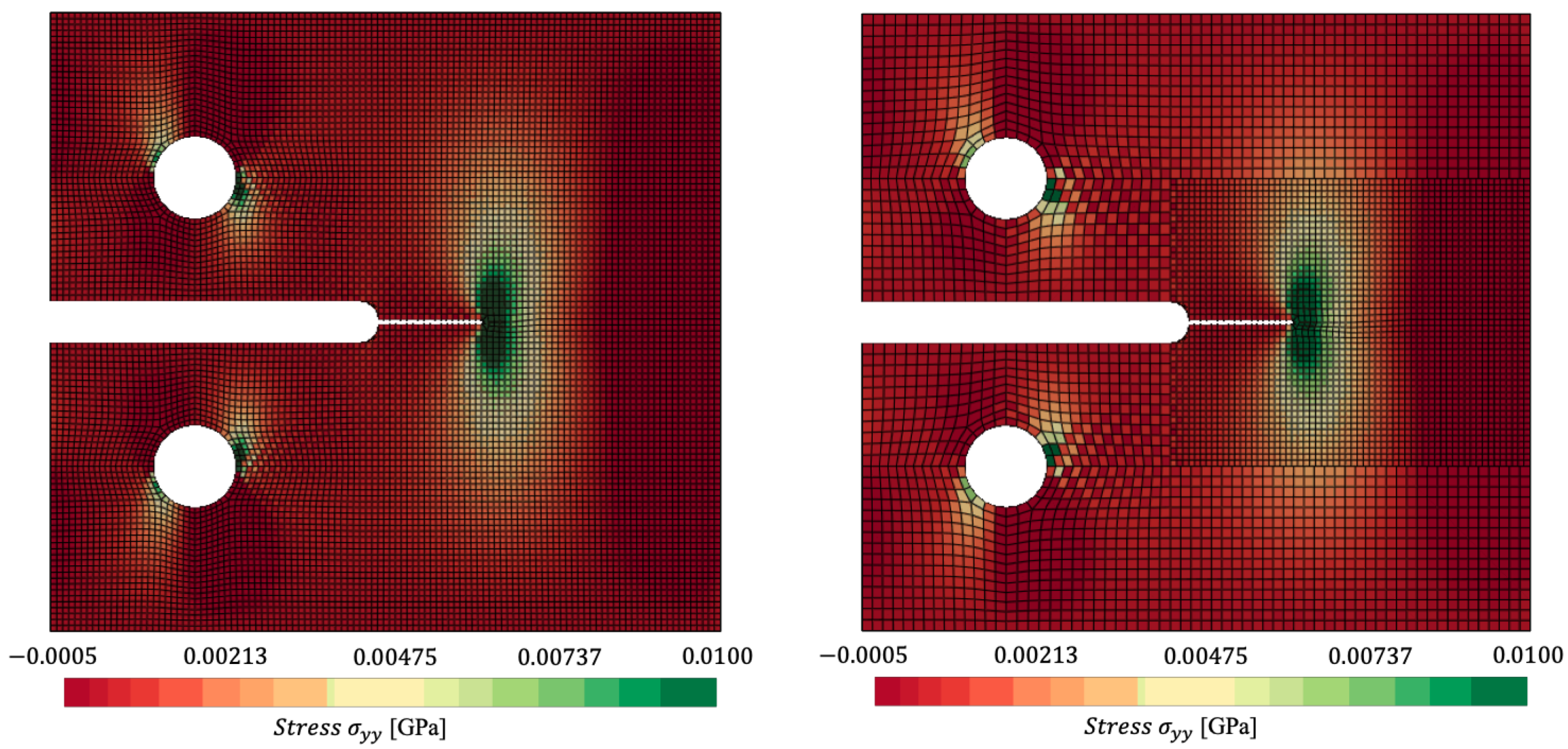
In Figure 7 and Figure 8 we plot the stress contours at ms and ms, respectively where the stress concentration can be visualised at the crack tip of the specimen. Figure 7 (a) and Figure 8 (a) capture the reference mesh, whilst Figure 7 (b) and Figure 8 (b) capture the spatially coupled mesh on a single time step . Figure 8 accurately predicts maximum stresses of 0.0396 GPa vs 0.0410 GPa for reference against non-matching mesh.
Through combining spatial and temporal coupling, we observe similar ( GPa) results in distribution, as seen in (a) of Figure 9. The difference in the coupled simulations is captured via the (b) of Figure 9, where the root mean square error (RMSE) is plotted. The stress is linear interpolated for the non-matching mesh, to allow for comparison of stress on the coarse mesh’s Gauss points. The couplings capture nearly the entire specimen within a % error. Considerable error is located around the circumference of the pins, and the far right of the specimen, however these Gauss points reside far from the area of interest at the crack tip. To avoid such errors, a smaller element size would be required in , however this raises the trade-off between accuracy and computational efficiency. Considerable speedup is achieved, with both couplings, as presented in Table 9.
Figure 9.
Comparison of for: (a) - combined spatial and temporal coupling (multi-time stepping); (b) - RMSE Error of for dynamically loaded compact-tension specimen at ms.
Figure 9.
Comparison of for: (a) - combined spatial and temporal coupling (multi-time stepping); (b) - RMSE Error of for dynamically loaded compact-tension specimen at ms.
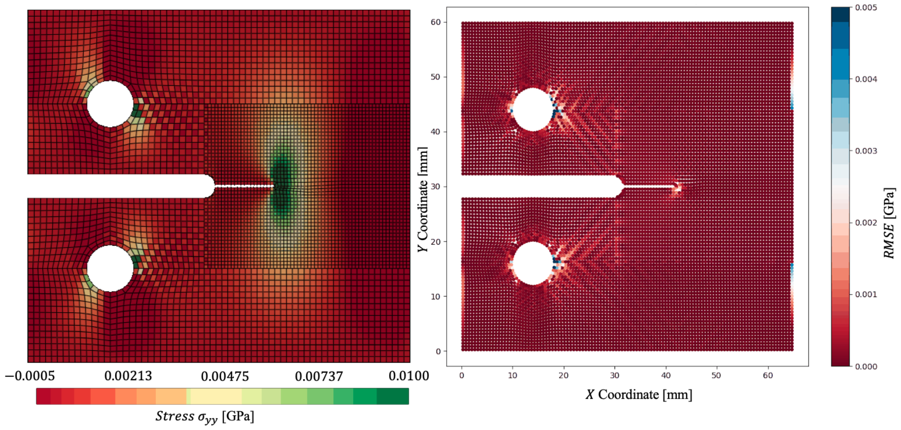

Table 1.
Computational runtime in seconds and speedup vs reference, of the dynamically loaded compact-tension specimen.
Table 1.
Computational runtime in seconds and speedup vs reference, of the dynamically loaded compact-tension specimen.
| Simulation | Runtime [s] | Speedup |
|---|---|---|
| Reference (monolithic) | 7428 | - |
| Spatially Coupled | 2267 | 3.27× |
| Spatially and Temporally Coupled | 572 | 12.98× |
5. Conclusions
We present coupling methods for the dynamic modelling of solids with explicit finite elements; temporally and spatially. When modelling composites, constituents have varying dilatational wave speeds, hence different time steps. Integrating over the smallest time step can prove highly inefficient, hence the need for multi-time stepping. Our method allows partitions of a domain to solve with their own respective time step, hence reducing computational overhead. Stability of the method is assessed through evaluation of the subdomains’ energies. The addition of the coupling in space solves the issue of non-matching meshes, so that small element sizes are only required in regions of interest. Coupling operators are easily implemented, without increasing the degrees of freedom on the interface. Ongoing work addresses the spatial coupling with a quadrilateral non-matching interfaces in 3-D domains [41]. Numerical examples capture an increase in efficiency with stress wave propagation in a heterogeneous bar, and the modelling of a compact-tension specimen. Both couplings in time and space reduce computational runtimes, when compared to their monolithic simulation, especially when combined. Future work looks at the coupling between macro and meso- scale meshes [42,43,44], with adaptivity a clear necessity for these multi-scale couplings [45]. Other coupling opportunities are plentiful when considering dynamic applications; the modelling of contact [14,16], composite fracture [38,39], fluid-structure interaction [13,27], and other impact engineering scenarios are just a few to mention.
Funding
This research was funded the Engineering and Physical Sciences Research Council (EPSRC) and Rolls-Royce’s ASiMoV Prosperity Partnership with Reference EP/S005072/1.
Data Availability Statement
The data that support the findings of this study are openly available upon request. The algorithm is described for two time-domains at https://github.com/kinfungchan/multi-time-step-integration.
Conflicts of Interest
The authors declare no conflicts of interest.
References
- Courant, R., Friedrichs, K. and Lewy, H., On the partial difference equations of mathematical physics. IBM journal of Research and Development 1967, 11(2), 215–234. [CrossRef]
- Hughes, T.J. and Liu, W.K., Implicit-explicit finite elements in transient analysis: Implementation and numerical examples. Journal of Applied Mechanics, Transactions ASME 1978, 45(2), 375–378. [CrossRef]
- Neal, M.O. and Belytschko, T., Explicit-explicit subcycling with non-integer time step ratios for structural dynamic systems. Computers & Structures 1989, 31(6), 871–880. [CrossRef]
- Daniel, W.J.T., Analysis and implementation of a new constant acceleration subcycling algorithm. International Journal for Numerical Methods in Engineering 1997, 40(15), 2841–2855.
- Daniel, W.J.T., A partial velocity approach to subcycling structural dynamics. Computer methods in applied mechanics and engineering 2003, 192(3-4), 375–394. [CrossRef]
- Lew, A., Marsden, J.E., Ortiz, M. and West, M., Variational time integrators. International Journal for Numerical Methods in Engineering 2004, 60(1), 153–212. [CrossRef]
- Combescure, A. and Gravouil, A., A numerical scheme to couple subdomains with different time-steps for predominantly linear transient analysis. Computer methods in applied mechanics and engineering 2002, 191(11-12), 1129–1157. [CrossRef]
- Gravouil, A., Combescure, A. and Brun, M., Heterogeneous asynchronous time integrators for computational structural dynamics. International Journal for Numerical Methods in Engineering 2015, 102(3-4), 202–232. [CrossRef]
- Cho, S.S., Kolman, R., González, J.A. and Park, K.C., Explicit multistep time integration for discontinuous elastic stress wave propagation in heterogeneous solids. International Journal for Numerical Methods in Engineering 2019, 118(5), 276–302. [CrossRef]
- Dvořák, R., Kolman, R., Mračko, M., Kopačka, J., Fíla, T., Jiroušek, O., Falta, J., Neuhäuserová, M., Rada, V., Adámek, V. and González, J.A., Energy-conserving interface dynamics with asynchronous direct time integration employing arbitrary time steps. Computer Methods in Applied Mechanics and Engineering 2023, 413, 116110. [CrossRef]
- de Boer, A., van Zuijlen, A.H. and Bijl, H., Review of coupling methods for non-matching meshes. Computer methods in applied mechanics and engineering 2007, 196(8), 1515–1525. [CrossRef]
- Hansbo, A. and Hansbo, P., An unfitted finite element method, based on Nitsche’s method, for elliptic interface problems. Computer methods in applied mechanics and engineering 2002, 191(47-48), 5537–5552. [CrossRef]
- Hansbo, A. and Hansbo, P., Nitsche’s method for coupling non-matching meshes in fluid-structure vibration problems. Computational Mechanics 2002, 32, 134–139. [CrossRef]
- Wriggers, P. and Zavarise, G., A formulation for frictionless contact problems using a weak form introduced by Nitsche. Computational Mechanics 2017, 41, 407–420. [CrossRef]
- Sanders, J.D., Laursen, T.A. and Puso, M.A., A Nitsche embedded mesh method. Computational Mechanics 2010, 49, 243–257. [CrossRef]
- Puso, M.A. and Laursen, T.A., A mortar segment-to-segment contact method for large deformation solid mechanics. Computer methods in applied mechanics and engineering 2004, 193(6-8), 601–629. [CrossRef]
- Faucher, V. and Combescure, A., A time and space mortar method for coupling linear modal subdomains and non-linear subdomains in explicit structural dynamics. Computer methods in applied mechanics and engineering 2003, 192(5-6), 509–533. [CrossRef]
- Steinbrecher, I., Mayr, M., Grill, M.J., Kremheller, J., Meier, C. and Popp, A., A mortar-type finite element approach for embedding 1D beams into 3D solid volumes. Computational Mechanics 2020, 66, 1377–1398. [CrossRef]
- Zhou, M., Zhang, B., Chen, T., Peng, C. and Fang, H., A three-field dual mortar method for elastic problems with nonconforming mesh. Computer Methods in Applied Mechanics and Engineering 2020, 362, 112870. [CrossRef]
- Wilson, P., Teschemacher, T., Bucher, P. and Wüchner, R., Non-conforming FEM-FEM coupling approaches and their application to dynamic structural analysis. Engineering Structures 2021, 241, 112342. [CrossRef]
- Singer, V., Teschemacher, T., Larese, A., Wüchner, R. and Bletzinger, K.U., Lagrange multiplier imposition of non-conforming essential boundary conditions in implicit material point method. Computational Mechanics 2024, 73(6), 1311–1333. [CrossRef]
- Puso, M.A. and Laursen, T.A., A simple algorithm for localized construction of non-matching structural interfaces. International Journal for Numerical Methods in Engineering 2002, 53(9), 2117–2142. [CrossRef]
- Herry, B., Di Valentin, L. and Combescure, A., An approach to the connection between subdomains with non-matching meshes for transient mechanical analysis. International Journal for Numerical Methods in Engineering 2002, 55(8), 973–1003. [CrossRef]
- Subber, W. and Matouš, K., Asynchronous space–time algorithm based on a domain decomposition method for structural dynamics problems on non-matching meshes Computational Mechanics 2016, 57, 211–235. [CrossRef]
- González, J.A., Kolman, R., Cho, S.S., Felippa, C.A. and Park, K.C., Inverse mass matrix via the method of localized Lagrange multipliers. International Journal for Numerical Methods in Engineering 2018, 113(2), 277–295. [CrossRef]
- Jeong, G.E., Song, Y.U., Youn, S.K. and Park, K.C., A new approach for nonmatching interface construction by the method of localized Lagrange multipliers. Computer Methods in Applied Mechanics and Engineering 2020, 361, 112728. [CrossRef]
- González, J.A. and Park, K.C., Three-field partitioned analysis of fluid–structure interaction problems with a consistent interface model. Computer Methods in Applied Mechanics and Engineering 2023, 414, 116134. [CrossRef]
- Cho, Y.S., Jun, S., Im, S. and Kim, H.G., An improved interface element with variable nodes for non-matching finite element meshes. Computer methods in applied mechanics and engineering 2005, 194(27-29), 3022–3046. [CrossRef]
- Kim, H.G., Development of three-dimensional interface elements for coupling of non-matching hexahedral meshes. Computer methods in applied mechanics and engineering 2005, 197(45-48), 3870–3882. [CrossRef]
- Bitencourt Jr, L.A., Manzoli, O.L., Prazeres, P.G., Rodrigues, E.A. and Bittencourt, T.N., A coupling technique for non-matching finite element meshes. Computer Methods in Applied Mechanics and Engineering 2015, 290, 19–44. [CrossRef]
- Rodrigues, E.A., Manzoli, O.L., Bitencourt Jr, L.A., Bittencourt, T.N. and Sánchez, M., An adaptive concurrent multiscale model for concrete based on coupling finite elements. Computer methods in applied mechanics and engineering 2018, 328, 26–46. [CrossRef]
- Dunne, F., and Petrinic, N., Introduction to computational plasticity, OUP Oxford, 2005.
- de Souza Neto, E.A., Peric, D. and Owen, D.R., Computational methods for plasticity: theory and applications, John Wiley & Sons, 2011.
- Belytschko, T., Liu, W.K., Moran, B. and Elkhodary, K., Nonlinear finite elements for continua and structures, John Wiley & Sons, 2014.
- Chan, K.F., Bombace, N., Sap, D., Wason, D., Falco, S. and Petrinic, N., A Multi-Time Stepping Algorithm for the Modelling of Heterogeneous Structures With Explicit Time Integration. International Journal for Numerical Methods in Engineering 2025, 126(1), e7638. [CrossRef]
- Biotteau, E., Gravouil, A., Lubrecht, A.A. and Combescure, A., Multigrid solver with automatic mesh refinement for transient elastoplastic dynamic problems. International Journal for Numerical Methods in Engineering 2010, 84(8), 947–971. [CrossRef]
- Dvořák, R., Kolman, R. and González, J.A., On the automatic construction of interface coupling operators for non-matching meshes by optimization methods. Computer Methods in Applied Mechanics and Engineering 2024, 432, 117336. [CrossRef]
- Pinho, S.T., Robinson, P. and Iannucci, L., Fracture toughness of the tensile and compressive fibre failure modes in laminated composites Composites Science and Technology 2006, 66(13), 2069–2079. [CrossRef]
- Sommer, D.E., Thomson, D., Hoffmann, J. and Petrinic, N., Numerical modelling of quasi-static and dynamic compact tension tests for obtaining the translaminar fracture toughness of CFRP. Composites Science and Technology 2023, 237, 109997. [CrossRef]
- Triclot, J., Corre, T., Gravouil, A. and Lazarus, V., Key role of boundary conditions for the 2D modeling of crack propagation in linear elastic Compact Tension tests. Engineering Fracture Mechanics 2023, 277, 109012. [CrossRef]
- Sahu, I., Bilinear-Inverse-Mapper: Analytical Solution and Algorithm for Inverse Mapping of Bilinear Interpolation of Quadrilaterals. 2024, Available at SSRN 4790071.
- Falco, S., Fogell, N., Iannucci, L., Petrinic, N. and Eakins, D., A method for the generation of 3D representative models of granular based materials. International Journal for Numerical Methods in Engineering 2017, 112(4), 338–359. [CrossRef]
- Wason, D., A multi-scale approach to the development of high-rate-based microstructure-aware constitutive models for magnesium alloys. Doctoral dissertation, University of Oxford.
- Falco, S., Fogell, N., Iannucci, L., Petrinic, N. and Eakins, D., Raster approach to modelling the failure of arbitrarily inclined interfaces with structured meshes. Computational Mechanics 2024, 74, 805-–818. [CrossRef]
- Bombace, N., Dynamic adaptive concurrent multi-scale simulation of wave propagation in 3D media. Doctoral dissertation, University of Oxford.
Figure 1.
A 3-D domain decomposed into and where and are non-matching interfaces to be externally resolved on . Normal vector and tractions are visualised on and respectively.
Figure 1.
A 3-D domain decomposed into and where and are non-matching interfaces to be externally resolved on . Normal vector and tractions are visualised on and respectively.
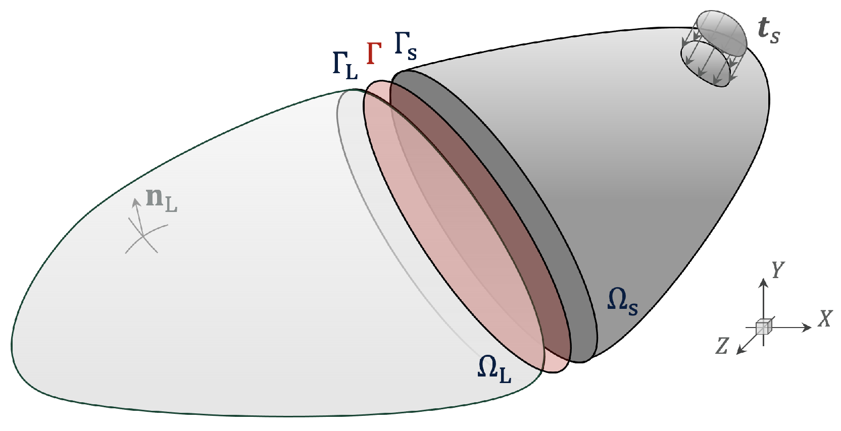
Figure 2.
A one-dimensional heterogeneous domain split into large subdomain and small subdomain , solved with and respectively, of length mm and mm The problem assuming uni-axial motion with . A compressive half sine velocity boundary condition is applied from .
Figure 2.
A one-dimensional heterogeneous domain split into large subdomain and small subdomain , solved with and respectively, of length mm and mm The problem assuming uni-axial motion with . A compressive half sine velocity boundary condition is applied from .
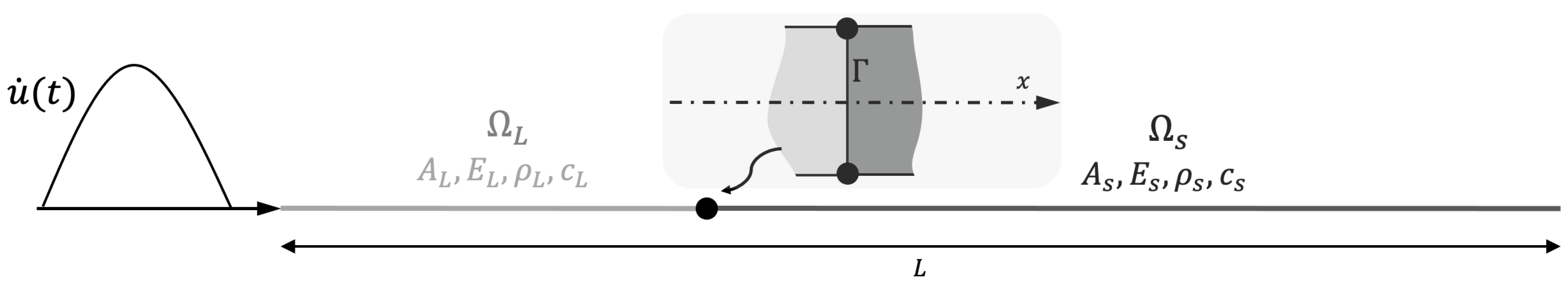
Figure 3.
Axial wave propagation in a heterogeneous bar: (a) - boundary condition at ms and initial transmission at ms of the stress wave; (b) - transmission and reflection of the stress wave at ms and ms.
Figure 3.
Axial wave propagation in a heterogeneous bar: (a) - boundary condition at ms and initial transmission at ms of the stress wave; (b) - transmission and reflection of the stress wave at ms and ms.
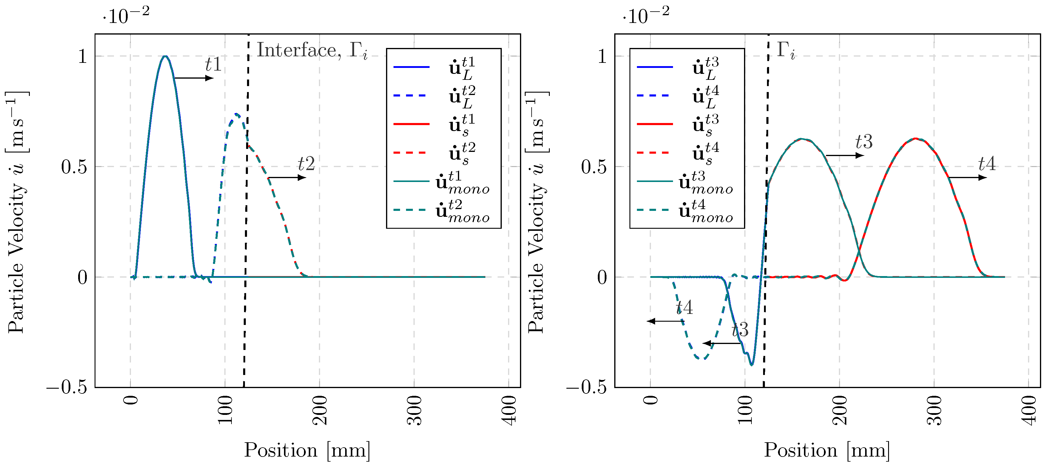
Figure 4.
Energy balance for axial wave propagation problem: (a) - Monolithic (single ) simulation system energy component history and balance with Equations 22 - 25, (b) - Multi-time stepping ( and ) simulation energy balance.
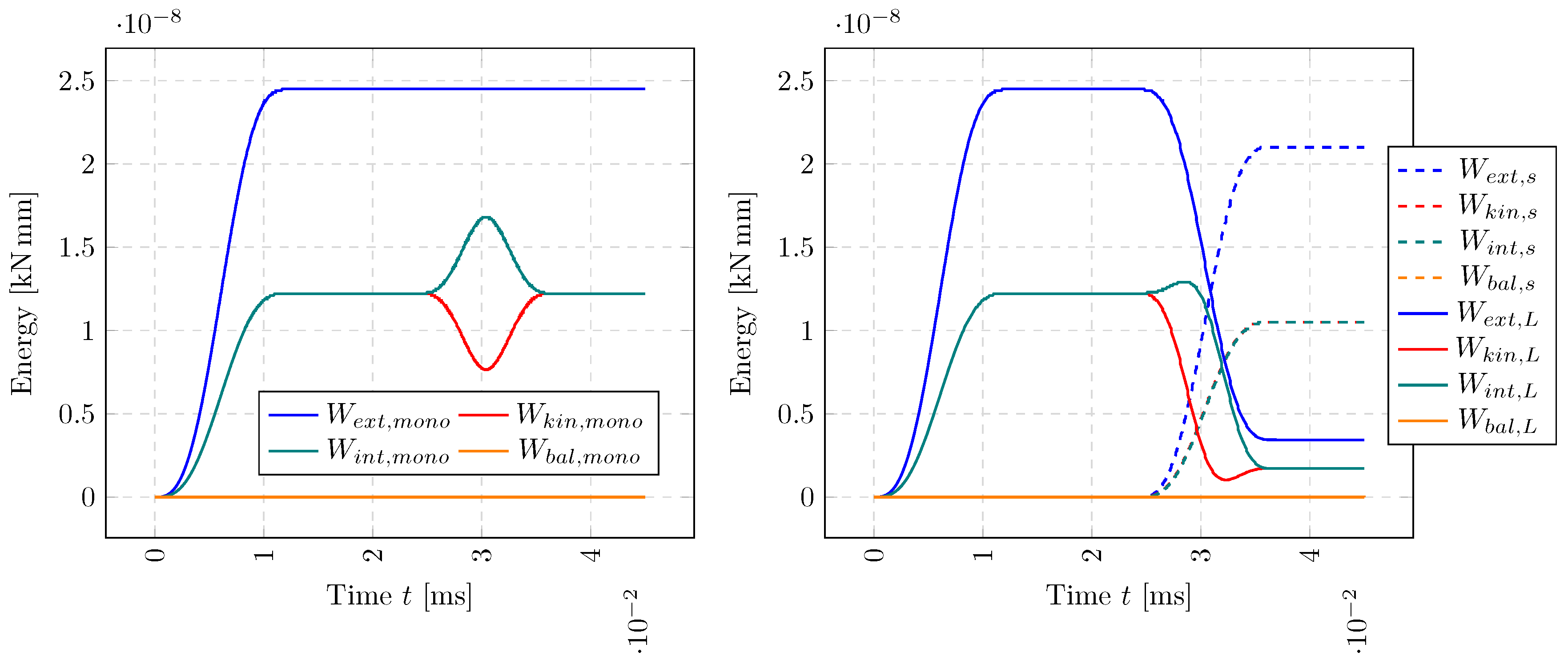
Figure 5.
A non-matching benchmark highlighting the interface with differently discretised subdomains partitioned with the Large , small and externally meshed interface .
Figure 5.
A non-matching benchmark highlighting the interface with differently discretised subdomains partitioned with the Large , small and externally meshed interface .
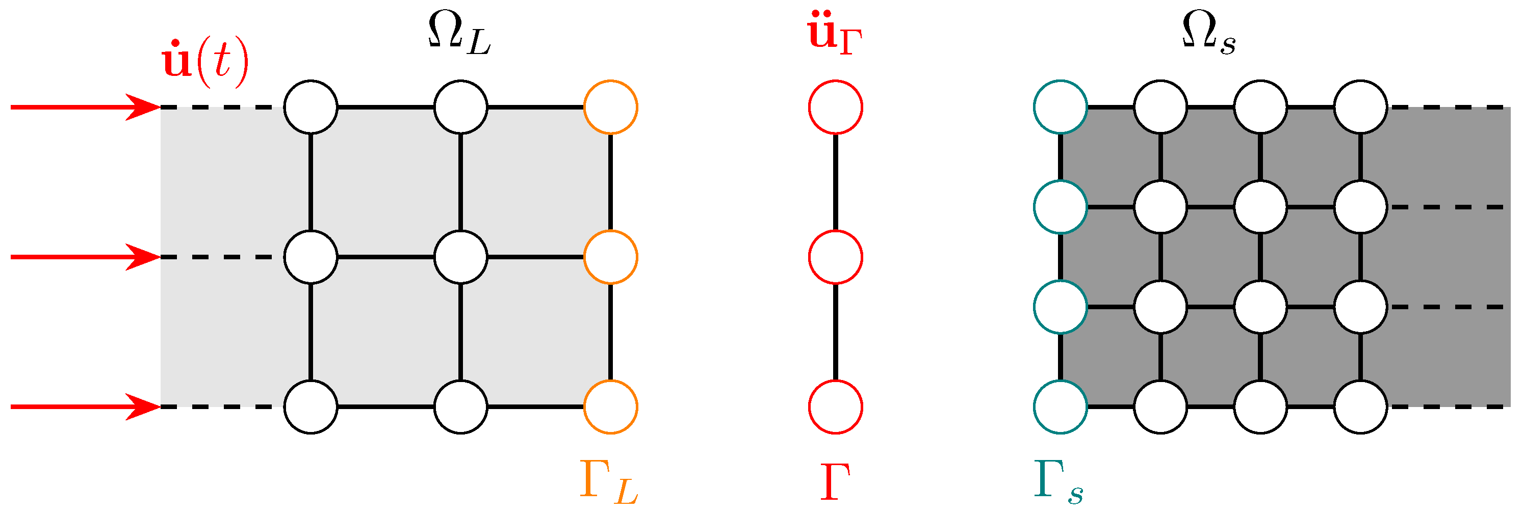
Figure 6.
(a) - Diagram of compact-tension specimen with dimensions in [mm], as seen in Sommer et al. [39]; (b) - Nodal sets on the meshed subdomain for prescribed velocity boundary conditions on top (+ve loading) and bottom (-ve loading) pins.
Figure 6.
(a) - Diagram of compact-tension specimen with dimensions in [mm], as seen in Sommer et al. [39]; (b) - Nodal sets on the meshed subdomain for prescribed velocity boundary conditions on top (+ve loading) and bottom (-ve loading) pins.
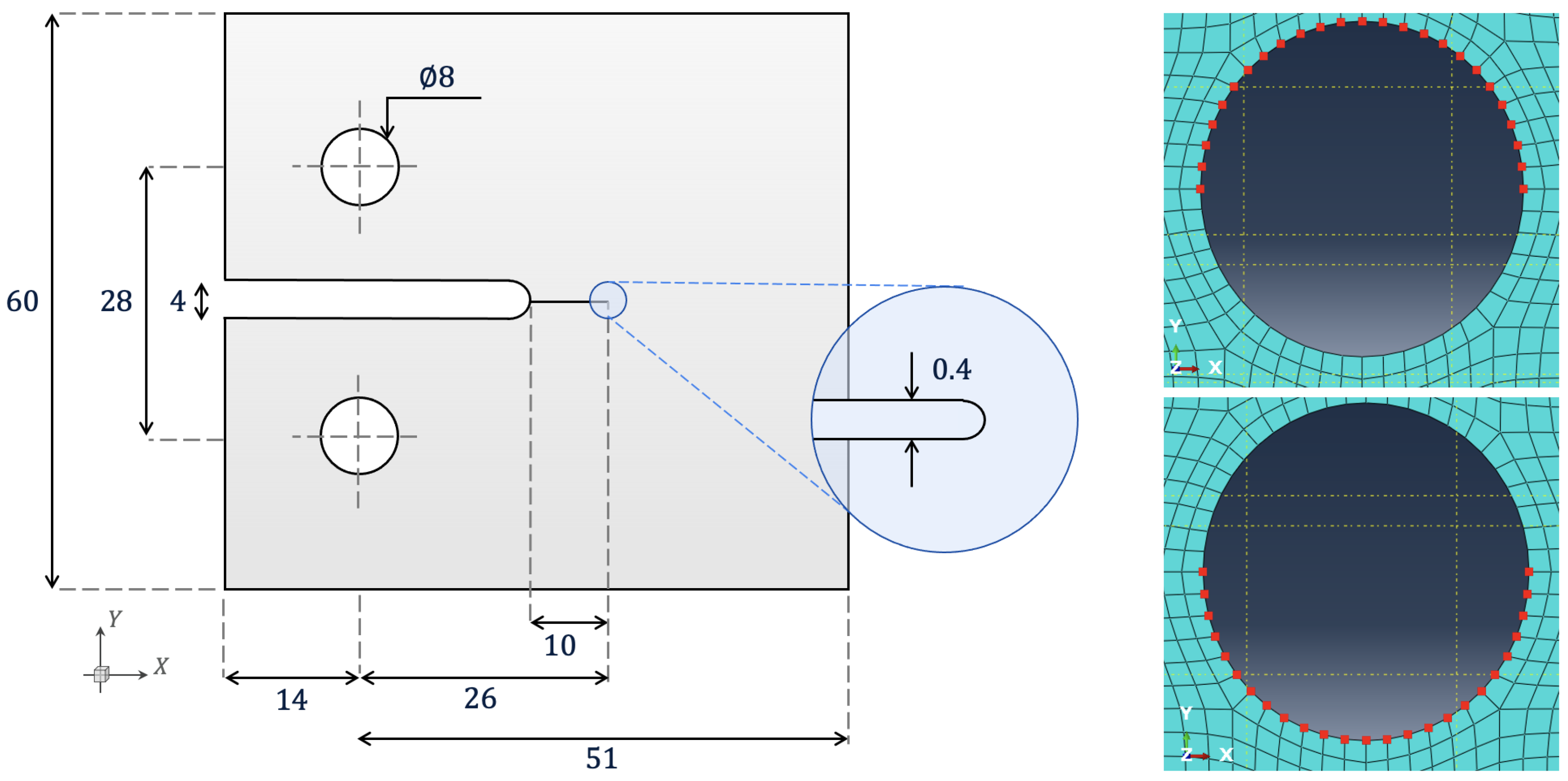
Figure 7.
Comparison of for: (a) - reference (monolithic) versus (b) - spatially coupled dynamically loaded compact-tension specimen, clipping from -0.0005 to 0.01 GPa at ms.
Figure 7.
Comparison of for: (a) - reference (monolithic) versus (b) - spatially coupled dynamically loaded compact-tension specimen, clipping from -0.0005 to 0.01 GPa at ms.
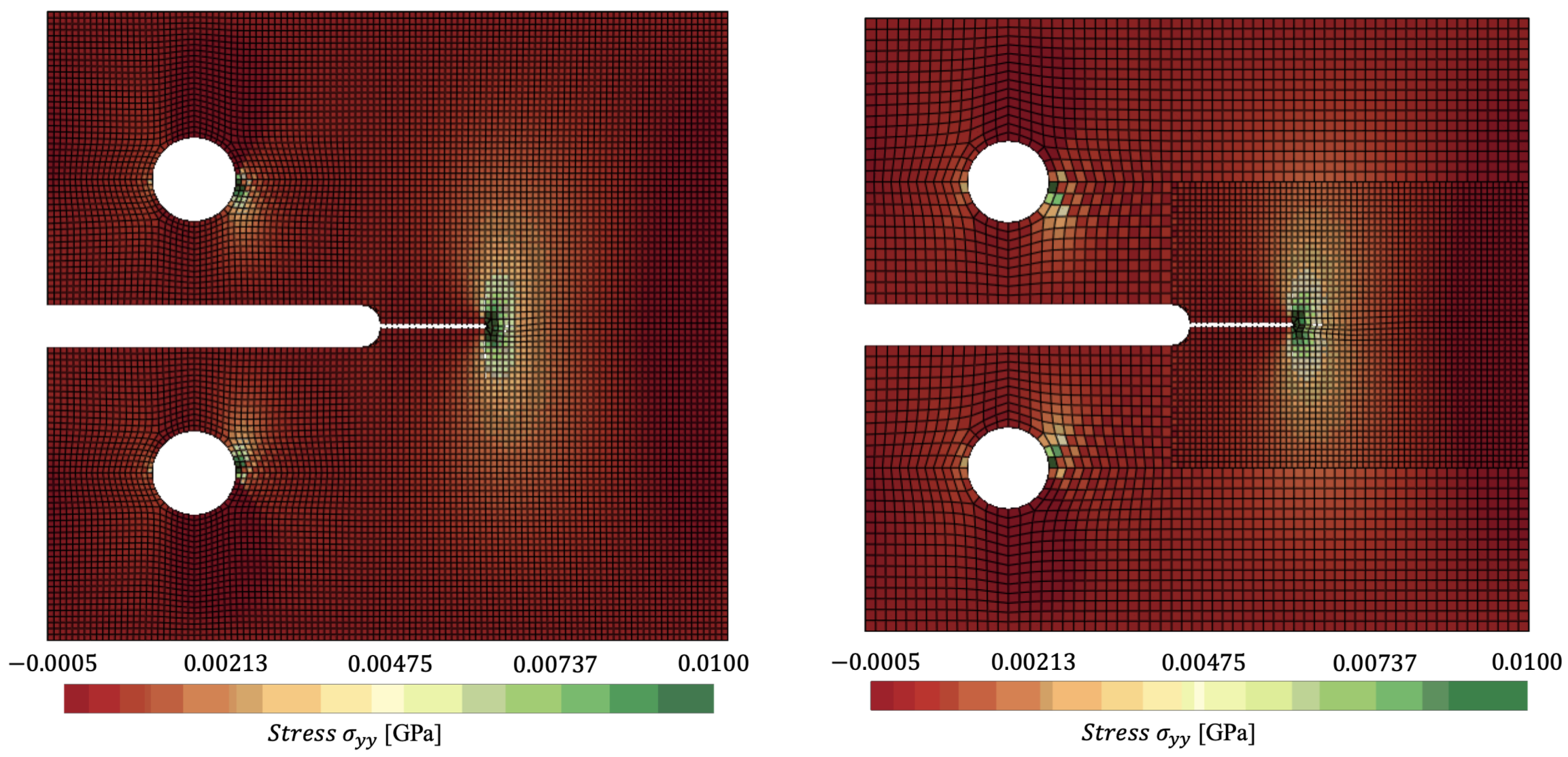
Figure 8.
Comparison of for: (a) - reference (monolithic) versus (b) - spatially coupled dynamically loaded compact-tension specimen, clipping from -0.0005 to 0.01 GPa at ms.
Figure 8.
Comparison of for: (a) - reference (monolithic) versus (b) - spatially coupled dynamically loaded compact-tension specimen, clipping from -0.0005 to 0.01 GPa at ms.
Disclaimer/Publisher’s Note: The statements, opinions and data contained in all publications are solely those of the individual author(s) and contributor(s) and not of MDPI and/or the editor(s). MDPI and/or the editor(s) disclaim responsibility for any injury to people or property resulting from any ideas, methods, instructions or products referred to in the content. |
© 2025 by the authors. Licensee MDPI, Basel, Switzerland. This article is an open access article distributed under the terms and conditions of the Creative Commons Attribution (CC BY) license (http://creativecommons.org/licenses/by/4.0/).
Copyright: This open access article is published under a Creative Commons CC BY 4.0 license, which permit the free download, distribution, and reuse, provided that the author and preprint are cited in any reuse.


