
Submitted:
05 February 2025
Posted:
05 February 2025
You are already at the latest version
Abstract
Background Prostate cancer management optimally requires non-invasive, objective, quantitative, accurate evalua-tion of prostate tumors. Current research applies visual inspection and quantitative approaches, such as artificial intelligence (AI) focused in deep learning (DL) to evaluate MRI. Recently, a different spectral/statistical approach successfully evaluated spatially registered bi-parametric MRIs for prostate cancer. This study aimed to further as-sess and improve the spectral/statistics approach through benchmarking and combining with AI.
Methods A zonal-aware self-supervised mesh network (Z-SSMNet) was applied to the same 42-patient cohort from previous spectral/statistical studies. The probability of clinical significance of prostate cancer (PCsPCa) and detec-tion map with affiliated tumor volume, eccentricity were computed for each patient. Linear and logistic regression were applied to International Society of Urological Pathology (ISUP) grade and PCsPCa, respectively. The R, p-value, Area Under the Curve (AUROC) from Z-SSMNet output was computed The Z-SSMNet output was combined with spectral/statistics output for multiple-variate regression.
Results The R (p-value), AUROC [95% Confidence Interval] from Z-SSMNet algorithm relating ISUP to PCsPCa is 0.298 (0.06), 0.50 [0.08-1.0], to average blob volume is 0.51 (0.0005), 0.37 [0.0-0.91], to total tumor volume is 0.36 (0.02), 0.50 [0.0-1.0]. R (p-value), AUROC computations showed much poorer correlation for eccentricity derived from Z-SSMNet detection map with ISUP. Overall DL/AI performed less well relative to spectral/statistical approaches from previous studies. Multi-variable regression fitted AI average blob size and SCR results in R=0.70 (0.000003) significantly higher than univariate regression fits of AI, spectral/statistics alone.
Conclusions. Spectral/statistical approaches performed well relative to Z-SSMNet. Combining Z-SSMNet with spectral/statistics approaches significantly enhanced tumor grade prediction, possibly providing an alternative to current prostate tumor assessment.
Keywords:
Prostate Cancer
; Bi-parametric MRI
; Spectral/statistics Approaches
; Deep Learning
; Artificial Intelligence
1. Introduction
Determining the prostate tumor’s potential for growth and metastases is essential for choosing whether a patient should undergo therapy or active surveillance [1,2,3,4,5,6]. Surgery, radiation therapy, and systemic therapy can control the disease but can also be physically, emotionally, and financially debilitating for the patient. Proper treatment choice may prolong life while preventing unnecessary side effects. MRI and ultrasound have been used to non-invasively evaluate the prostate with minimal side effects [11,12,13,14]. MRI is particularly sensitive for detecting prostate cancers. MRI scanning generates structural (T2) and functional (diffusion, dynamic contrast enhancement) images that can offer additional insight into the aggressiveness of the tumor [15,16,17,18,19]. Trained radiologists visually inspect the prostate tumor and assess the patient based on specific scoring systems such as PI-RADS [20,21]. In practice, visual inspection of MRI can be inconsistent, and accurate assessment depends on the experience and training of a given radiologist [21,22]. Although injecting contrast reveals the tumor vasculature and provides valuable information, reducing patient inconvenience and simplifying and expediting clinical flow motivate foregoing the contrast scan by scanning with only two parameters (Apparent Diffusion Coefficient, DWI (High-B Value), T2), also known as bi-parametric (BP) MRI [24,25,26,27,28,29,30,31].
Instead of relying on the radiologist’s subjective judgement, quantitative approaches, such as deep learning (DL) and artificial intelligence (AI) algorithms [32,33,34], are applied to BP-MRI to expedite the analysis and aid the radiologist. The DL and AI models were trained on large-scale datasets of the patients to capture spatial features such as textures for predicting tumor aggressiveness. There has been great interest in DL and AI throughout technology and science, especially in examining MRI for prostate cancer assessment [32,33,34]. To help sort through the plethora of DL and AI algorithms, a PI-CAI Grand Challenge [35,36,37,38] evaluated 293 DL and AI algorithms trained on a common BP-MRI dataset of publicly available 1,500 cases from 1476 patients that had tissue confirmation of the diagnosis . Each of the candidate algorithms produced tumor detection maps and the probability of clinical significance for prostate cancer for each patient. The competing algorithms were evaluated based on an additional, common test set of independent patient data. In particular, a Z-SSMNet algorithm composed of Yuan et al. from Australia [38] achieved a top performing algorithm status in the PI-CAI Grand Challenge for accurate prostate tumor evaluation and detection.
Recently, spectral/statistical techniques have been applied to spatially registered multi- and bi- parametric MRI [39,40,41,42,43,44] to assess prostate cancer. The techniques were adapted from processing hyperspectral imagers mounted on airborne platforms. Instead of extracting and employing spatial features such as used in DL and AI, the spectral/statistics identify tumors through spectral signatures, analogous to spectroscopic studies and human color vision, require minimal training and can be adapted to different clinical conditions. The pilot studies demonstrated that features such as Signal to Clutter Ratio [39,42,43], tumor volume [42,44], and tumor eccentricity [42,44] correlated with tumor grade and showed promise in terms of their ability to assess prostate cancer. Although the Area Under the Curve (AUROC) derived from Receiver Operator Characteristic (ROC) curve from the spectral/statistical approaches in previous pilot studies have generally not inferior to AI, those studies did not directly compare AI and spectral/statistical approaches at the patient-to-patient level [39,40,41,42,43,44].
DL and AI that primarily exploit spatial features such as textures differ substantially from spectral/statistics approaches. These differences may mean that the DL/AI and spectral/statistics approaches are uncorrelated with each other. Combining spatial and spectra approaches may potentially boost tumor grade prediction, analogous to human vision and its ability to detect and evaluate a given scene.
2. Materials and Methods
This is a retrospective study to compare two approaches for assessing prostate cancer from bi-parametric MRI. The novel techniques employed are summarized below with greater detail in prior reports and small-cohort pilot studies [38,39,40,41,42,43,44]. Some details are also summarized in later sections of this approach.
2.1. Overall Approach
Figure 1 shows the overall scheme to compare a metric related to the Gleason score, namely the International Society of Urological Pathology (ISUP) grade [45] and Clinically Significant (Insignificant) Prostate Cancer or CsPCa (CiPCa) with metrics generated from spatially registered MRI, namely z-score and processed Signal to Clutter Ratio (SCR) [39,42,43] (green highlighted panel), eccentricity (red highlighted panel), and tumor volume (blue highlighted panel). In addition, an AI approach was applied to the same data(yellow panel). ISUP grade is determined from PI-CAI pathology analysis [45] of the histopathology slides from MRI-directed biopsy (MRBx), Systematic Biopsy (SysBx), the combination of MRBx and SysBx, and radical prostatectomy (RP) (Figure 1. label A). For this study, patient MRI data and their assessments were gathered as part of the PI-CAI Grand Challenge [35,36,37,38] (Figure 1. label A, B). In the BP-MRI arm [39,40,41,42,43,44] of the study, spatially registered vectorial 3D image to the voxel level are assembled from the individual MRI sequences, specifically the Apparent Diffusion Coefficient (ADC), High B-Value (HBV) from the Diffusion Weighted Images (DWI), and T2 by translating, resizing the images (Figure 1. label C). Using the spatially registered MRI, the prostate is manually outlined to generate a normal prostate mask (Figure 1. label D), input for covariance matrix computation (Figure 1. label E). In-scene signatures (Figure 1. label F) are derived from the spatially registered vectorial 3D image to provide input for the z-score and SCR computation [39,42]. Noise in the SCR [39,42] is reduced through principal component filtering, regularizing the covariance matrix (Figure 1. label G). The processed SCR and z-score are linearly (logistical probability) fitted to the ISUP grade (CsPCa/CiPCa), respectively (Figure 1. label H, green hashed arrows). Metrics describing the linear and logistic fits are given by the correlation coefficients (R) and the AUROC from Receiver Operator Characteristic (ROC) [39,40,41,42,43,44].
Figure 1 also summarizes the procedures for generating the eccentricity and tumor volume measurements. Adaptive Cosine Estimator (ACE) detection calculations (Figure 1, label ‘I’), thresholding (Figure I, label ‘J’’ and ‘N’) and prostate volume calculations (Figure 1, label “K”,”L”) and prostate tumor eccentricity (Figure 1, label “O”,”P”) and linear regression and logistic probability fits (Figure 1, label ‘M’) to the ISUP, CsPCa from biopsy (Figure 1 label ‘P’). Direction of output data to be used as input denoted by arrows. Red arrows and box indicate eccentricity calculations from BP- MRI-based data; blue arrows and box denote tumor volume estimated from bi-parametric MRI.
The spatial registration of the bi-parametric data, processing, and calculations of SCR, ROC curve, and AUROC were executed using the Python 3 programming language, scikit-learn, numpy, panda libraries.
In addition, a Deep Learning approach entitled Z-SSMNet (Zonal-aware Self-supervised Mesh Network) by Yuan et al. [38] was applied to the same 42 patient cohort. The 42 patients resided in the validation set of fold0 designated by the PI-CAI [36]. The Z-SSMNet algorithm was trained on the rest data composed of the validation set of fold1, fold2, fold3, fold4 to generate weights (Figure 1, label “R”) in order to infer likelihood and detection maps for the 42 patients (Figure 1, label “S”). These inferred values were used in the regression fits (Figure 1, label “T”).
Figure 2 shows a specific example taken from patient 10085 in the PI-CAI data collect. The figures show spatially registered slices that have been stitched together. Selected stitched sections of ADC, High-B-Value, and T2 files were assigned red, green, blue colors, respectively, in the color composite. A threshold (set to 0.9) stitched selection from Adaptive Cosine Estimator (ranges from 0.0 to 1.0) and labeled blobs and their volume and eccentricity. In addition, Figure 2 shows the volumes and eccentricity for the blobs from Z-SSMNet (Yuan) detection map.
2.2. Study Design and Population
MRI and assessments were collected and stored through PI-CAI [35,36,37]. The PI-CAI challenge stores an annotated multi-center, multi-vendor publicly available dataset of 1500 BP-MRI exams that includes clinical and acquisition variables. Various histopathology techniques were used [35,36], but only a subset of the 1500-patient study underwent or had available biopsy results. Patients were scanned at a variety of centers and assorted Siemens and Philips scanners. The PI-CAI data collection [35,36] only includes bi-parametric MRI, namely ADC, HBV, and T2 sequences.
Previously, 42 consecutive patients who had been biopsied in the PI-CAI database were assessed. All patients had biopsy-proven adenocarcinoma of the prostate, with a mean patient age of 65.1 years (range, 50 to 78 years), a mean PSA of 13.49 ng/mL (range, 1.5 to 81.95 ng/mL), mean prostate volume of 60.6 cm3 (range 19 to 192 cm3), and mean ISUP grade of 1.12 (range, 0 to 5), 31(11) cases were confirmed as clinically insignificant (significant) prostate cancer. This study placed no restrictions on tumor location within the prostate. Informed consent was exempted due to the retrospective nature of this study. All cases were anonymized for subsequent analysis.
2.3. Spatial Registered Vectorial 3D Image Assembly: Magnetic Resonance Imaging
2.4. Spatial Registered Vectorial 3D Image Assembly: Image Processing, Pre-Analysis
Before applying spatial registration, the spatial resolution and spatial offsets for the scanning setup of a given patient were read from image header files for each of the MRI sequences (ADC, HBV, and T2). The MRI images were digitally resized [39,40,41,42,43,44] to the sequence with the lowest spatial resolution in the transverse direction. Using the offsets listed in the image header files, the images were translated a few pixels (or no pixels) to the reference image (ADC and HBV)). Based on the known location of the axial offsets, the slices were selected and resampled to match the offsets. Also, small transverse translation adjustments, based on visual inspection, were applied to the T2 image to match the appropriate ADC and HBV slices.
A “cube” is composed of stacked individual slices that had been appropriately scaled, translated, cropped, and spatially registered at the voxel level. Following cropping, all images shared the common field of view (FOV). These “three dimensional” (two transverse directions plus spectral dimension composed of ADC, HBV, and T2 images) cubes were “stitched” together into a narrow three-dimensional vectorial image cube to depict the entire body within the common field of view of the MRI scan. This stitching of MRI slices (or mosaicking) emulates configurations used in remote sensing, in which small patches are stitched together into large swaths of areas, thereby increasing the processing speed to handle large, high dimensional data. Spatial registration for each patient took a few seconds to process on a Windows 10, Base Speed 2 Ghz, Cache memory 8 Gbyte machine. The registration was visually inspected. Sometimes small translations (1 voxel) corrections were applied to for individual slices correctly spatially register the BP-MRI and cropping to ensure common size for all slices within the stack.
2.5. Overall Quantitative Metrics Description: SCR, Z-Score
In medical practice, trained radiologists visually inspect multiple MRI images to qualitatively determine a tumor aggressiveness [22,23]. In contrast, the SCR and z-score are quantitative metrics denoting a tumors’ departure from normal prostate tissue. The z-score and SCR formulation combine information from all BP-MRI sequences. SCR and z-score compute the difference between the mean tumor signature value and the mean normal prostate value, scaled by the normal prostate standard deviation for each MRI sequence (ADC, HBV, and T2). However, z-score does not account for correlation among the BP-MRI sequences (ADC, HBV, and T2). Instead, the SCR decorrelates the sequences by whitening the spatially registered BP-MRI. In the whitening process, noise is added. The SCR computation requires computing the covariance matrix that ultimately corrects for correlations among the different sequences (i.e., the correlation between ADC and DWI) and thereby determines the true contribution of each sequence. References [39,40,41,42,43,44] summarizes the mathematics behind the SCR algorithm. For each patient, SCR calculations took a few seconds to process on a Windows 10, base speed 2 Ghz, cache memory 8 Gbyte machine.
2.6. SCR: Filtering Noise
The covariance matrix for the SCR can be decomposed into principal components (PC) [47]. Principal components are linear combinations of all MRI components. The principal components are orthogonal to each other and, therefore, decorrelated. Conventionally, the principal components ordering is based on their eigenvalue or statistical variation. The high eigenvalue (low PC number) PC image displays high variation within the image. In contrast, noisy images (high PC number) are associated with principal components having small eigenvalues and low variation within the image. Filtering and eliminating the noisy (low eigenvalue, high PC number) principal components reduces noise from inverting the covariance matrix and increases the SCR calculation accuracy. References [39,40,41,42,43,44,48] summarizes the mathematics for filtering principal components.
2.7. Regularization and Shrinkage
Regularization [40,43,49] results from the constraints on the coefficients in the Langrangian optimization process. In this application, regularization also ensures that the covariance matrix follows a normal distribution. The analytic formula only approximates the covariance matrix. Shrinkage regularization [40,43,49] perturbs the original covariance matrix CM(γ) by mixing a diagonal matrix with an adjustable parameter γ to generate a regularized or modified regularized covariance matrix. The appropriate γ minimizes the discriminant function and thereby more appropriately mimic the normal distribution. Regularized and modified regularized covariance matrix calculations follow the same procedure but differ in their choice of the mixing diagonal matrix. References [40,43,49] summarizes the mathematics behind regularization procedures.
2.8. Logistic Regression
A logistic regression fit [50] results from fitting processed SCR, z-score, patient data, Z-SSMNet likelihood scores to the dependent categorical variable CsPCa. The ISUP grade is taken from biopsy. The clinically significant PCa (CsPCa) was assigned to ISUP grade ≥ 2. The clinically insignificant PCa (CiPCa) was assigned to <2. New randomized sets were generated 1000 times forming configurations of patients within the training/test sets, generating 1000 ROC [51] curves and resulting in a distribution of AUROC. The distribution of AUROC scores was recorded, along with the 2.5% and 97.5% largest AUROC delineated the 95% confidence interval. The fit quality was assessed through the AUROC and the 95% confidence interval from the ROC curves.
2.9. Adaptive Cosine Estimator (ACE) Algorithm
The Adaptive Cosine Estimator (ACE) algorithm is a supervised target detection algorithm [38,39,40,41,42,43,51]. Supervised target detection algorithms [39,40,41,42,43,44,52] peruse and classify a voxel into either a target (prostate tumor) or background (normal prostate) based on information about the target (tumor), specifically the tumor signature. The tumor signature S is a three-dimensional vector whose components are intensity values within the manifold (ADC, High B Value, T2) that characterize the target. The background is characterized by a mean three-dimensional vector m and covariance matrix CM (3 dimensions X 3 dimensions) that includes the variance and accounts for correlations among the different dimensions. A multi-dimensional (3-D for BP-MRI) cone is centered around the target signature S. The ACE decision surface follows this cone. Voxels whose ACE scores residing within the decision cone are assigned to the target. Voxels residing outside the cone are assigned to the background. References [39,40,41,42,43,44,52] offers a more detailed summary of the ACE algorithm and clarifying equations.
2.10. Tumor Volume Measurements, Supervised Target Detection
To compute a metric associated with the tumor volume, the ACE algorithm was applied to the spatially registered BP-MRI [41,42,44]. Voxels that lie inside the decision cone or exceed a threshold for ACE scores were assigned to the tumor. Normal tissue was assigned to voxels that resided outside the decision cone or had ACE scores residing below the threshold. The number of voxels exceeding a given threshold were counted and assigned to be tumor. This sum is converted to volume based on the MRI spatial resolution. References [41,42,44] summarizes the mathematics behind the tumor volume computation.
2.11. Labeling and Blob Generation
Within computer vision, connected component labeling or blobbing and labeling [41,42,44] refer to the process of objectively aggregating neighboring voxels. The blobbing is applied to a mask image or binary image following the application of a threshold to the ACE detection image. The values of 1 or 0, or “True” or “False,” are associated with the tumor (background) in each masked image. Each “True” voxel peruses voxels within a given neighborhood (1 voxel away) to see if they are also “True.” Blobbing is associated with an 8-pixel connected neighborhood involving the “True,” “1,” or “Tumor” voxels in the masked image. If the “True” are connected, the particular voxels are collected and labeled as a member of a blob. Blobs smaller than 5 voxels (~10−2 mL) were filtered out.
2.12. Eccentricity Calculation
Custom software coded in Python 3 calculated the eccentricity [41,42,44] for every labeled blob. Following the identification of a blob, the moment of inertia matrix I for the kth blob was computed. The eigen equation (using the moment of inertia I) was solved, resulting in computing the eigenvalues for each blob.. The largest eigenvalue was assigned to the large axis lk,, and the second eigenvalue was assigned to the transverse moment sk. The eccentricity Ek for the kth blob is a normalized difference of the major axis lk and minor axis sk. Eccentricity values Ek range from 0 (spherical shape) to 1 (line). Reference [40,41,43] offers a more detailed summary of the eccentricity computation and clarifying equations.
2.13. Machine Learning Application: Z-SSMNet
This study directly compares the findings of spectral/statistical techniques with the application of a publicly available trained AI models derived from a highly performing program as judged in the recent PI-CAI Challenge [35,36,37,38]. Specifically, this study examined and applied the Zonal-aware Self-supervised Mesh Network (Z-SSMNet) algorithm developed by Yuan et al. from Australia [38].
The Z-SSMNet algorithm [38] used axial-plane image sequences from BP-MRI PI-CAI dataset. No clinical variables from routine practice (patient age, PSA, prostate volume) nor acquisition variables (MRI scanner manufacturer, vendor, scanner, model, b-value of the diffusion weighted imaging etc.) associated with the imaging were employed to guide the prediction. The Z-SSMNet algorithm ameliorated some issues that plague DL resulting in improved performance. Current state-of-the-art AI algorithms are often based on deep learning for 2D images that fail to capture inter-slice correlations in 3D volumetric images. 3D convolutional neural networks (CNNs) partly overcome this deficiency. However, 3D CNN does not handle the anisotropy within images and can introduce artifacts. In addition, due to the limited amount of labelled data of BP-MRI and labelling difficulties, CNNs employ relatively small datasets, leading to poor performance. To address these limitations, a new Z-SSMNet model deployed on the 3D nnU-Net framework [53] to help learn region-specific high-level semantic information, zonal specific domain knowledge, (whole gland or the transitional and peripheral zones), to constrain the computation and improve the diagnostic precision for csPCa and reduce false positive detection. The new method adaptatively fuses multiple 2D/2.5D/3D CNNs following the U-Net architecture) [54] and accommodates for both sparse inter-slice information and dense intra-slice information in BP-MRI. In addition, a self-supervised learning (SSL) technique extracts textures and boundary information and pre-trains the unlabelled data in order to extract the generalizable image features. Experiments on the PI-CAI Challenge BP-MRI datasets show high performance for csPCa detection and diagnosis. The AUROC and Average Precision (AP) scores are 0.890 and 0.709 in Hidden Validation and Tuning Cohort (100 cases) (2nd rank) and 0.881 and 0.633 in Hidden Testing Cohort (1000 cases) (1st rank), respectively.
The Z-SSMNet algorithm [38] computes a suspicion score (single floating-point value between 0-1) for a given patient representing the likelihood that a patient harbors a clinically significant cancer. The relationship between CsPCa likelihood and ISUP is unclear. The ISUP grades 0, 2, 5 should correspond to probabilities of 0., 0.5, 1.0 respectively. In addition to recording Z-SSMNet’s likelihood scores for each patient, this study inferred the ISUP from interpolating linear relationship. Figure 3 plots the inferred ISUP grades against the probability of CsPCa and shows the known fixed points (blue filled circles) and the patient values derived from linear interpolation. This study also interpolated patient values based on ISUP=3.6409*tanh-1 (Probability) where 3.6409 is chosen so that probability=0.5 corresponds to ISUP=2.
The 42 cases analyzed using the spectral/statistics approach were extracted from the validation set of fold0 (semi-supervised setting) in the PI-CAI Challenge. The weights for the inference were based on the model trained on the rest of the data composed of the validation set of fold1, fold2, fold3, fold4.
2.14. Univariate and Multivariate Fitting
One or multiple independent variables are fitted to a single independent variable using univariate and multivariate linear regression analysis, respectively [55,56]. In this study, the independent variables correspond to an individual (such as largest) and collective (such as average or weighted) blob eccentricity, blob volume derived from a fixed, thresholds, Signal to Clutter Ratio (PC filtered, Regularized) ACE, and likelihood scores from Z-SSMNet. The dependent variable is the ISUP grade or CsPCa. The latter is a categorical variable (binary variable or either True or False). The fits minimize the error in a least squares calculation by finding the optimal fitting coefficient for the independent variable. These fitting coefficients can be applied to the independent variables to generate a fit, which are then compared to actual data. Correlation coefficients and fitted lines test the agreement of the computed p values to assess the probability that the fit is or is not correlated. Confidence Intervals are computed for every variable along with p values for the multivariable fit. Reference [27] offers a more detailed summary of the linear regression fitting and provides clarifying equations.
Tumor aggressiveness or CsPCa estimation might be improved (beyond univariate regression) by applying linear multi-variate [55,56] or logistic probability regression (Methods, 2.8) [50] to the combination of AI approach with spectral/statistical algorithms. Previously [21,22], SCR combined with tumor eccentricity, volume increased the correlation coefficient, AUROC.
3. Results
Yuan’s algorithm generates likelihood scores and detection maps. Figure 4 plots a variety of measures derived from the Z-SSMNet algorithm computed from each patient such as the likelihood and from the computed detection map. Processing of the detection map generated a number of features, specifically, the number of blobs, eccentricity from the largest blob, average eccentricity, mass weighted eccentricity, maximum blob volume, average blob volume, total tumor volume. The likelihood and the detection maps features were plotted against the ISUP score derived from biopsy. From linear regression, the correlation coefficient (R) and p-value are also shown in the figure. Unlike spectra/statistical approaches, the AI derived tumor eccentricity was not a good predictor of prostate tumor aggressiveness.
The Z-SSMNet likelihood and features derived from the detection map was plotted and fitted through linear regression to the ISUP score for each patient in the 42-patient cohort. The R (p-value) and AUROC [95% Confidence Interval] from Z-SSMNet (Yuan) algorithm relating ISUP to PCsPCa is 0.298 (0.06) and 0.50 [0.08-1.0], to average blob volume is 0.51 (0.0005) and 0.37 [0.0-0.91], to total tumor volume is 0.36 (0.02) and 0.50 [0.0-1.0], to eccentricity (maximum blob) is 0.0 (0.96), to eccentricity (average) is 0.14 (0.38), to eccentricity (weighted) is 0.06 (0.73). From earlier studies, the R (p-value) from spectral/statistics approach relating ISUP score to processed SCR ranged from 0.55 to 0.58 (<<0.02), to tumor volumes from 0.37 to 0.42 (0.018 to 0.03) and 0.70 to 0.95 [0.33-1.0], to tumor eccentricity (largest blob) from 0.35 to 0.37 (0.01 to 0.015) and 0.44 to 0.90 [0.12-1.0]. Generally, the R and AUROC values from the Z-SSMNet algorithm are lower than those from spectral/statistical approaches.
Table 1 summarizes the best performing univariate linear regression from Z-SSMNet predictors to ISUP.
AI derived features and spectral/statistical features were combined in multi-variable fitting to ISUP. The best performing multivariate linear regression fits are summarized in Table 2. The biggest increase in correlation occurs for features that mix AI and spectral/statistical approaches, which also has the lowest cross-correlation coefficient from mixing AI and spectral/statistical approaches. Note, combining z-score and SCR (modified Regularization) from spectral/statistics approach shows high univariate R1, R2, and also high cross correlation, but poor R12 relative to the combinations that mix AI and Spectral/Statistics approaches. AI average blob size and SCR results in R-0.70, p<0.02, significantly higher than multiple regression fits involving AI or Spectral/statistics alone. Combining spectral/statistics approach derived eccentricity (maximum blob) or average blob volume, or maximum blob with Z-SSMNet derived average blob in a multi-variate fit to ISUP resulted in minimal increases in correlation coefficient (R12) due to relatively poor univariate correlation (R1, R2) and high cross correlation among the tumor volume measures. Previously, univariate logistic fits of z-score, processed SCR from spectral/statistics achieved AUROC scores of 1.0[1.0-1.0] [43] resulting in similar AUROC scores for multi-variate logistic fits that include SCR derived from the spectral/statistics approach.
Figure 5 plots the individual patient data as well as the calculated multi-variate fits taken from the average blob derived from AI (Z-SSMNet) and the Modified Regularized SCR from spectral/statistical approach against the ISUP derived from biopsy.
4. Discussion
This is the first study to directly compare and combine DL/AI algorithms and spectral/statistics approaches on a per- patient basis. This retrospective pilot study of 42 patients from the PI-CAI data collect shows that the new spectral/statistics approach demonstrates performance at least comparable to an DL/AI algorithm for achieving high correlation with tumor grade and accurately predicting clinically significant prostate cancer. The high performance of spectral/statistics approaches is notable due to its simplicity in conception, calculation, application and understanding relative to AI Unlike spectral/statistics approaches, the eccentricity from the DL/AI algorithm detection map did not show anti-correlation with prostate tumor grade. Based on the results of this pilot study, further studies to confirm these promising results regarding the relative efficacy of individually spectral/statistics approach and AI and the combination of the two approaches are warranted.
Studies of adenocarcinoma morphologies of breast cancer [57] and lung cancer [58,59] show that the tumors become more symmetric as the tumor grade increases or adenocarcinoma eccentricity is anti-correlated with tumor grade. Recently [41,42,43,44], evidence has been gathered that prostate cancer, nearly always an adenocarcinoma, also is anti-correlated with tumor grade. The recent studies [41] examined outlined histopathology slides from prostatectomy, spectral/statistical approaches applied to 26 patients with multi-parametric MRI and bi-parametric MRI. In this study, DL/AI found that tumor grade correlated with tumor volume but did not correlate with tumor eccentricity or shape. The detection maps generated by the models in the PI-CAI challenges may not accurately predict the tumor region as the evaluation criterion is that the overlap between the predicted tumor and the true value exceeds 0.1. The DL/AI algorithms may further benefit by incorporating training using tumor morphology, such as tumor volume and eccentricity instead of confining their training to spatial textures for predicting clinical significance of prostate cancer.
This study only analyzed 42 consecutive patients. All the studied patients resided in the PI-CAI fold0 among 5 folds cross-validation study in the PI-CAI Grand Challenge. Although the calculated p-values for correlating the ISUP and the 95% confidence intervals for the AUROC in the ROC curves, additional independent study using a higher number of patients are needed to meaningfully confirm the results.
This study confined its analysis to only one DL/AI algorithm, namely the Z-SSMNet algorithm by Yuan et al. from Australia [38]. The Z-SSMNet algorithm achieved second place (among 293 algorithms) in the PI-CAI Grand-Challenge assessment. There is no evidence that the choice of the Z-SSMNet algorithm achieves a performance inconsistent with other high achieving performers in the Grand-Challenge. Nevertheless, future studies should process the selected patient cohort with additional AI algorithms.
For multi-variate regression fitting, combining DL/AI with spectral/statistics approaches achieves higher correlation with tumor grade than separately applying regression involving DL/AI or spectral/statistics. Note the low correlation coefficient, meaning less replication and possibly more synergy among algorithms that are distinctly different. Further investigations into the combined use of DL/AI and spectral/statistics approaches are warranted with larger number of patients and employing other DL/AI algorithms.
Human vision employs both spatial and spectral features to detect and discriminate among targets. This study showed that combining spatial and spectral approaches can be especially effective in determining prostate tumor aggressiveness. Emulating vision (or possibly human-ideation-driven approaches), instead of intelligence, may prove a more fruitful avenue for improving algorithmic performance for analyzing prostate tumors depicted in MRI.
5. Conclusions
This first pilot retrospective study compared and combined prostate tumor assessments from DL/AI algorithms with spectral/statistics approaches. Spectral/statistical approaches performed well relative to DL. Combining AI with spectral/statistics approaches significantly enhanced tumor grade prediction.
Author Contributions
Conceptualization, R.M., Y.Y.; methodology, R.M., Y.Y.; software, R.M. Y.Y.; validation, R.M., Y.Y.; formal analysis, R.M. .; investigation, R.M. Y.Y.; resources, Y.Y.; data curation, R.M., Y.Y. ; writing—original draft preparation, R.M.; writing—review and editing, R.M., Y.Y., J.U., B.T., P.C., D.H., H.L, C.S.; visualization, R.M..; supervision, R.M. Y.Y., J.U., P.C., C.S. ; project administration, R.M. Y.Y., J.U., P.C., C.S. ; funding acquisition.
Funding
This research received no external funding.
Institutional Review Board Statement
The data collect and AI analysis was conducted in accordance with the Declaration of Helsinki, and approved by the Institutional Review Board and regional review boards of each participating centers (Prostaat Centrum Noord-Nederland: IRB 2018–597; St Olav’s Hospital, Trondheim University Hospital: REK 2017/576; Radboud University Medical Center: CMO 2016–3045; and Ziekenhuisgroep Twente: ZGT 23–37).
Informed Consent Statement
Informed consent was exempted due to the retrospective nature of this study.
Data Availability Statement
The data presented in this study are available in PI-CAI Grand-Challenge at https://pi-cai.grand-challenge.org/DATA/ Additional raw data supporting the conclusions of this article will be made available by the authors on request
Acknowledgments
Dr Yuan Yuan is thanked for permitting access to his calculations resulting from applying the Z-SSMNet algorithm to selected patients within the PI-CAI data collect. Dr Yubing Tong is thanked for his help.
Conflicts of Interest
The authors declare no conflicts of interest.
Abbreviations
The following abbreviations are used in this manuscript:
| SSA | Spectral/Statistics Approach |
| SCR | Signal to Clutter Ratio |
| ACE | Adaptive Cosine Estimator |
| AUROC | Area Under the Curve |
| AP | Average Precision |
| BP-MRI | Bi-parametric MRI |
| CsPCa | Clinically Significant Prostate Cancer |
| ROC | Receiver Operator Characteristic |
| Mod Reg | Modified Regularization |
| Reg | Regularization |
| PC | Principal Component |
| DL | Deep Learning |
| AI | Artificial Intelligence |
| ISUP | International Society Urological Pathology |
| PI-RADS | Prostate Imaging Reporting and Data System |
| PI-CAI | Prostate Imaging Artificial Intelligence |
| Z-SSMNet | Zonal-Aware Self-Supervised Mesh Network |
References
- Papachristodoulou A, Abate-Shen C. Precision intervention for prostate cancer: Re-evaluating who is at risk. Cancer Lett. 2022 Jul 10;538:215709. [CrossRef] [PubMed]
- Parker, C.; Castro, E.; Fizazi, K.; Heidenreich, A.; Ost, P.; Procopio, G.; Tombal, B.; Gillessen, S. Prostate cancer: ESMO Clinical Practice Guidelines for diagnosis, treatment and follow-up. Ann. Oncol. 2020, 31, 1119–1134. [Google Scholar] [CrossRef] [PubMed]
- Wang T, Lewis B, Ruscetti M, Mittal K, Wang MJ, Sokoloff M, Ding L, Bishop-Jodoin M, FitzGerald TJ. Prostate Cancer: Advances in Radiation Oncology, Molecular Biology, and Future Treatment Strategies. In: Barber N, Ali A, editors. Urologic Cancers [Internet]. Brisbane (AU): Exon Publications; 2022 Sep 12. Chapter 13. [PubMed]
- Williams IS, McVey A, Perera S, O'Brien JS, Kostos L, Chen K, Siva S, Azad AA, Murphy DG, Kasivisvanathan V, Lawrentschuk N, Frydenberg M. Modern paradigms for prostate cancer detection and management. Med J Aust. 2022 Oct 17;217(8):424-433. [CrossRef] [PubMed]
- Ziglioli F, Granelli G, Cavalieri D, Bocchialini T, Maestroni U. What chance do we have to decrease prostate cancer overdiagnosis and overtreatment? A narrative review. Acta Biomed. 2019 Dec 23;90(4):423-426. [CrossRef] [PubMed]
- Zuur LG, de Barros HA, van der Mijn KJC, Vis AN, Bergman AM, Pos FJ, van Moorselaar JA, van der Poel HG, Vogel WV, van Leeuwen PJ. Treating Primary Node-Positive Prostate Cancer: A Scoping Review of Available Treatment Options. Cancers (Basel). 2023 May 29;15(11):2962. [CrossRef] [PubMed]
- Zattoni F, Rajwa P, Miszczyk M, Fazekas T, Carletti F, Carrozza S, Sattin F, Reitano G, Botti S, Matsukawa A, Dal Moro F, Jeffrey Karnes R, Briganti A, Novara G, Shariat SF, Ploussard G, Gandaglia G. Transperineal Versus Transrectal Magnetic Resonance Imaging-targeted Prostate Biopsy: A Systematic Review and Meta-analysis of Prospective Studies. Eur Urol Oncol. 2024 Dec;7(6):1303-1312. [CrossRef] [PubMed]
- Zhou M, Epstein JI. The reporting of prostate cancer on needle biopsy: prognostic and therapeutic implications and the utility of diagnostic markers. Pathology. 2003 Dec;35(6):472-9. [CrossRef] [PubMed]
- Bloemberg J, de Vries M, van Riel LAMJG, de Reijke TM, Sakes A, Breedveld P, van den Dobbelsteen JJ. Therapeutic prostate cancer interventions: a systematic review on pubic arch interference and needle positioning errors. Expert Rev Med Devices. 2024 Jul;21(7):625-641. [CrossRef] [PubMed]
- Zhu M, Liang Z, Feng T, Mai Z, Jin S, Wu L, Zhou H, Chen Y, Yan W. Up-to-Date Imaging and Diagnostic Techniques for Prostate Cancer: A Literature Review. Diagnostics (Basel). 2023 Jul 5;13(13):2283. [CrossRef] [PubMed]
- Fernandes MC, Yildirim O, Woo S, Vargas HA, Hricak H. The role of MRI in prostate cancer: current and future directions. MAGMA. 2022 Aug;35(4):503-521. [CrossRef] [PubMed]
- Tricard T, Garnon J, Cazzato RL, Al Hashimi I, Gangi A, Lang H. "Prostate management" under MRI-guidance: 7 years of improvements. Transl Cancer Res. 2020 Apr;9(4):2280-2286. [CrossRef] [PubMed]
- Triquell M, Campistol M, Celma A, Regis L, Cuadras M, Planas J, Trilla E, Morote J. Magnetic Resonance Imaging-Based Predictive Models for Clinically Significant Prostate Cancer: A Systematic Review. Cancers (Basel). 2022 Sep 29;14(19):4747. [CrossRef] [PubMed]
- Würnschimmel C, Chandrasekar T, Hahn L, Esen T, Shariat SF, Tilki D. MRI as a screening tool for prostate cancer: current evidence and future challenges. World J Urol. 2023 Apr;41(4):921-928. [CrossRef] [PubMed]
- Kamsut S, Reid K, Tan N. Roundtable: arguments in support of using multi-parametric prostate MRI protocol. Abdom Radiol (NY). 2020 Dec;45(12):3990-3996. [CrossRef] [PubMed]
- Stabile, A.; Giganti, F.; Rosenkrantz, A.B.; Taneja, S.S.; Villeirs, G.; Gill, I.S.; Allen, C.; Emberton, M.; Moore, C.M.; Kasivisvanathan, V. Multiparametric MRI for prostate cancer diagnosis: Current status and future directions. Nat. Rev. Urol. 2020, 17, 41–61. [Google Scholar] [CrossRef] [PubMed]
- Ursprung S, Herrmann J, Nikolaou K, Harland N, Bedke J, Seith F, Zinsser D. Die multiparametrische MRT der Prostata: Anforderungen und Grundlagen der Befundung [Multiparametric MRI of the prostate: requirements and principles regarding diagnostic reporting]. Urologie. 2023 May;62(5):449-458. German. [CrossRef] [PubMed]
- Zhao Y, Simpson BS, Morka N, Freeman A, Kirkham A, Kelly D, Whitaker HC, Emberton M, Norris JM. Comparison of Multiparametric Magnetic Resonance Imaging with Prostate-Specific Membrane Antigen Positron-Emission Tomography Imaging in Primary Prostate Cancer Diagnosis: A Systematic Review and Meta-Analysis. Cancers (Basel). 2022 Jul 19;14(14):3497. [CrossRef] [PubMed]
- Ziglioli F, Maestroni U, Manna C, Negrini G, Granelli G, Greco V, Pagnini F, De Filippo M. Multiparametric MRI in the management of prostate cancer: an update-a narrative review. Gland Surg. 2020 Dec;9(6):2321-2330. [CrossRef] [PubMed]
- Scott R, Misser SK, Cioni D, Neri E. PI-RADS v2.1: What has changed and how to report. SA J Radiol. 2021 Jun 1;25(1):2062. [CrossRef] [PubMed]
- Spilseth B, Margolis DJA, Gupta RT, Chang SD. Interpretation of Prostate Magnetic Resonance Imaging Using Prostate Imaging and Data Reporting System Version 2.1: A Primer. Radiol Clin North Am. 2024 Jan;62(1):17-36. [CrossRef] [PubMed]
- Annamalai A, Fustok JN, Beltran-Perez J, Rashad AT, Krane LS, Triche BL. Interobserver Agreement and Accuracy in Interpreting mpMRI of the Prostate: a Systematic Review. Curr Urol Rep. 2022 Jan;23(1):1-10. [CrossRef] [PubMed]
- Taya M, Behr SC, Westphalen AC. Perspectives on technology: Prostate Imaging-Reporting and Data System (PI-RADS) interobserver variability. BJU Int. 2024 Oct;134(4):510-518. [CrossRef] [PubMed]
- Padhani, A.R.; Schoots, I.; Villeirs, G. Contrast Medium or No Contrast Medium for Prostate Cancer Diagnosis. That Is the Question. J. Magn. Reson. Imaging. 2021, 53, 13–22. [Google Scholar] [CrossRef] [PubMed]
- Palumbo P, Manetta R, Izzo A, Bruno F, Arrigoni F, De Filippo M, Splendiani A, Di Cesare E, Masciocchi C, Barile A. Biparametric (bp) and multiparametric (mp) magnetic resonance imaging (MRI) approach to prostate cancer disease: a narrative review of current debate on dynamic contrast enhancement. Gland Surg. 2020 Dec;9(6):2235-2247. [CrossRef] [PubMed]
- Pecoraro M, Messina E, Bicchetti M, Carnicelli G, Del Monte M, Iorio B, La Torre G, Catalano C, Panebianco V. The future direction of imaging in prostate cancer: MRI with or without contrast injection. Andrology. 2021 Sep;9(5):1429-1443. [CrossRef] [PubMed]
- Scialpi M, D'Andrea A, Martorana E, Malaspina CM, Aisa MC, Napoletano M, Orlandi E, Rondoni V, Scialpi P, Pacchiarini D, Palladino D, Dragone M, Di Renzo G, Simeone A, Bianchi G, Brunese L. Biparametric MRI of the prostate. Turk J Urol. 2017 Dec;43(4):401-409. [CrossRef] [PubMed]
- Scialpi M, Martorana E, Scialpi P, D'Andrea A, Torre R, Di Blasi A, Signore S. Round table: arguments in supporting abbreviated or biparametric MRI of the prostate protocol. Abdom Radiol (NY). 2020 Dec;45(12):3974-3981. [CrossRef] [PubMed]
- Steinkohl F, Pichler R, Junker D. Short review of biparametric prostate MRI. Memo. 2018;11(4):309-312. [CrossRef] [PubMed]
- Tamada, T.; Kido, A.; Yamamoto, A.; Takeuchi, M.; Miyaji, Y.; Moriya, T.; Sone, T. Comparison of Biparametric and Multiparametric MRI for Clinically Significant Prostate Cancer Detection with PI-RADS Version 2.1. J. Magn. Reason. Imaging 2021, 53, 283–291. [Google Scholar] [CrossRef] [PubMed]
- Twilt JJ, van Leeuwen KG, Huisman HJ, Fütterer JJ, de Rooij M. Artificial intelligence based algorithms for prostate cancer classification and detection on magnetic resonance imaging: a narrative review. Diagnostics. 2021 May 26;11(6):959.
- Baltzer PAT, Clauser P. Applications of artificial intelligence in prostate cancer imaging. Curr Opin Urol. 2021 Jul 1;31(4):416-423. [CrossRef] [PubMed]
- Zhao LT, Liu ZY, Xie WF, Shao LZ, Lu J, Tian J, Liu JG. What benefit can be obtained from magnetic resonance imaging diagnosis with artificial intelligence in prostate cancer compared with clinical assessments? Mil Med Res. 2023 Jun 26;10(1):29. [CrossRef] [PubMed]
- Zhu L, Pan J, Mou W, Deng L, Zhu Y, Wang Y, Pareek G, Hyams E, Carneiro BA, Hadfield MJ, El-Deiry WS, Yang T, Tan T, Tong T, Ta N, Zhu Y, Gao Y, Lai Y, Cheng L, Chen R, Xue W. Harnessing artificial intelligence for prostate cancer management. Cell Rep Med. 2024 Apr 16;5(4):101506. [CrossRef] [PubMed]
- Saha, A.; Twilt, J.J.; Bosma, J.S.; Van Ginneken, B.; Yakar, D.; Elschot, M.; Veltman, J.; Fütterer, J.; de Rooij, M.; Huisman, H. Artificial Intelligence and Radiologists at Prostate Cancer Detection in MRI: The PI-CAI Challenge (Study Protocol). Available online: https://zenodo.org/record/6624726#.ZGvT2nbMKM9 (accessed on 28 April 2023).
- Saha, A et al. Artificial intelligence and radiologists in prostate cancer detection on MRI (PI-CAI): an international, paired, non-inferiority, confirmatory study The Lancet Oncology, 2024 Volume 25, Issue 7, 879 – 887.
- Saha, A et al. Appendix Artificial intelligence and radiologists in prostate cancer detection on MRI (PI-CAI): an international, paired, non-inferiority, confirmatory study The Lancet Oncology, 2024 Volume 25, Issue 7.
- Yuan Y, Ahn E, Feng, D, Khadra M, Kim J.. Z-SSMNet: A Zonal-aware Self-Supervised Mesh Network for Prostate Cancer Detection and Diagnosis in bpMRI. 10.48550/arXiv.2022 2212.05808.
- Mayer, R.; Simone CB 2nd Skinner, W.; Turkbey, B.; Choyke, P. Pilot study for supervised target detection applied to spatially registered multiparametric MRI in order to non-invasively score prostate cancer. Comput. Biol. Med. 2018, 94, 65–73. [Google Scholar] [CrossRef] [PubMed]
- Mayer, R.; Simone, C.B., 2nd; Turkbey, B.; Choyke, P. Development and testing quantitative metrics from multi-parametric magnetic resonance imaging that predict Gleason score for prostate tumors. Quant. Imaging Med. Surg. 2022, 12, 1859–1870. [Google Scholar] [CrossRef] [PubMed]
- Mayer, R.; Turkbey, B.; Choyke, P.; Simone, C.B., 2nd. Combining and Analyzing Novel Multi-parametric MRI Metrics for Predicting Gleason Score. Quant. Imaging Med. Surg. 2022, 12, 3844–3859. [Google Scholar] [CrossRef] [PubMed]
- Mayer, R.; Turkbey, B.; Choyke, P.; Simone, C.B., 2nd. Pilot Study for Generating and Assessing Nomograms and Decision Curves Analysis to Predict Clinically Significant Prostate Cancer Using Only Spatially Registered Multi-Parametric MRI. Front. Oncol. Sec. Genitourin. Oncol. 2023, 13, 1066498. [Google Scholar] [CrossRef]
- Mayer R, Turkbey B, Choyke PL, Simone CB II. Application of Spectral Algorithm Applied to Spatially Registered Bi-Parametric MRI to Predict Prostate Tumor Aggressiveness: A Pilot Study. Diagnostics, 2023 13, 2008. [CrossRef]
- Mayer R, Turkbey B, Choyke PL, Simone CB, II. Relationship between Eccentricity and Volume Determined by Spectral Algorithms Applied to Spatially Registered Bi-Parametric MRI and Prostate Tumor Aggressiveness: A Pilot Study. Diagnostics 2023 13, 3238. [CrossRef]
- Egevad, L.; Delahunt, B.; Srigley, J.R.; Samaratunga, H. International Society of Urological Pathology (ISUP) grading of prostate cancer—An ISUP consensus on contemporary grading. APMIS 2016, 124, 433–435. [Google Scholar] [CrossRef] [PubMed]
- Ahdoot, M.; Wilbur, A.R.; Reese, S.E.; Lebastchi, A.H.; Mehralivand, S.; Gomella, P.T.; Bloom, J.; Gurram, S.; Siddiqui, M.; Pinsky, P.; et al. MRI-Targeted, Systematic, and Combined Biopsy for Prostate Cancer Diagnosis. N. Engl. J. Med. 2020, 382, 917–928. [Google Scholar] [CrossRef] [PubMed]
- Strang, G. Linear Algebra and Its Applications, 4th ed.; Thomson, Brooks/Cole: Belmont, CA, USA, 2006.
- Chen, G.; Qian, S. Denoising of Hyperspectral Imagery Using Principal Component Analysis and Wavelet Shrinkage. IEEE Trans. Geosci. Remote Sens. 2011, 49, 973–80. [Google Scholar] [CrossRef]
- Friedman, J.H. Regularized Discriminant Analysis. J. Am. Stat. Assoc. 1989, 84, 165–7. [Google Scholar] [CrossRef]
- Hosmer, D.W., Jr.; Lemeshow, S.; Sturdivant, R.X. Applied Logistic Regression, 2nd ed.; Wiley: Hoboken, NJ, USA, 2000; ISBN 978-0-471-35632-5. [Google Scholar]
- Fawcett, T. An Introduction to ROC Analysis. Pattern Recognit. Lett. 2006, 27, 861–874. [Google Scholar] [CrossRef]
- Manolakis D, Shaw G, Detection algorithms for hyperspectral imaging applications, IEEE Sign. Processing Magazine. 2002; 19: 29-43.
- Isensee F, Jaeger PF, Kohl SAA et al., “nnU-Net: a self-configuring method for deep learning-based biomedical image segmentation,” Nature Methods, 2021 vol. 18, no. 2, 203-+.
- . Dong, Y. He, X. Qi et al., “MNet: Rethinking 2D/3D Networks for Anisotropic Medical Image Segmentation,” 2022. arXiv:2205.04846, 2022.
- Mardia KV, Kent JT, Bibby JM. Multivariate Analysis. Academic Press, 1979.
- Chatterjee S, Simonoff J. Handbook of Regression Analysis. Hoboken: John Wiley & Sons, 2013.
- Bae MS, Seo M, Kwang, Kim KG, Park IA, Moon WK. Quantitative MRI morphology of invasive breast cancer: correlation with immunohistochemical biomarkers and subtypes. Acta Radiol. 2015 Mar;56(3):269-75. [CrossRef]
- Yoon HJ, Park H, Lee HY, Sohn I, Ahn J and Lee SH. Prediction of tumor doubling time of lung adenocarcinoma using radiomic margin characteristics. Thoracic Cancer 2020; 11: 2600–2609.
- Baba T, Uramoto H, Takenaka M, et al..The tumour shape of lung adenocarcinoma is related to the postoperative prognosis. Interactive CardioVascular and Thoracic Surgery. 2012; 15: 73–76.
Figure 1.
Schematic showing the overall process for calculating features from spectral/statistics approaches and Yuan's algorithm and their relationship to ISUP and detection map.
Figure 1.
Schematic showing the overall process for calculating features from spectral/statistics approaches and Yuan's algorithm and their relationship to ISUP and detection map.
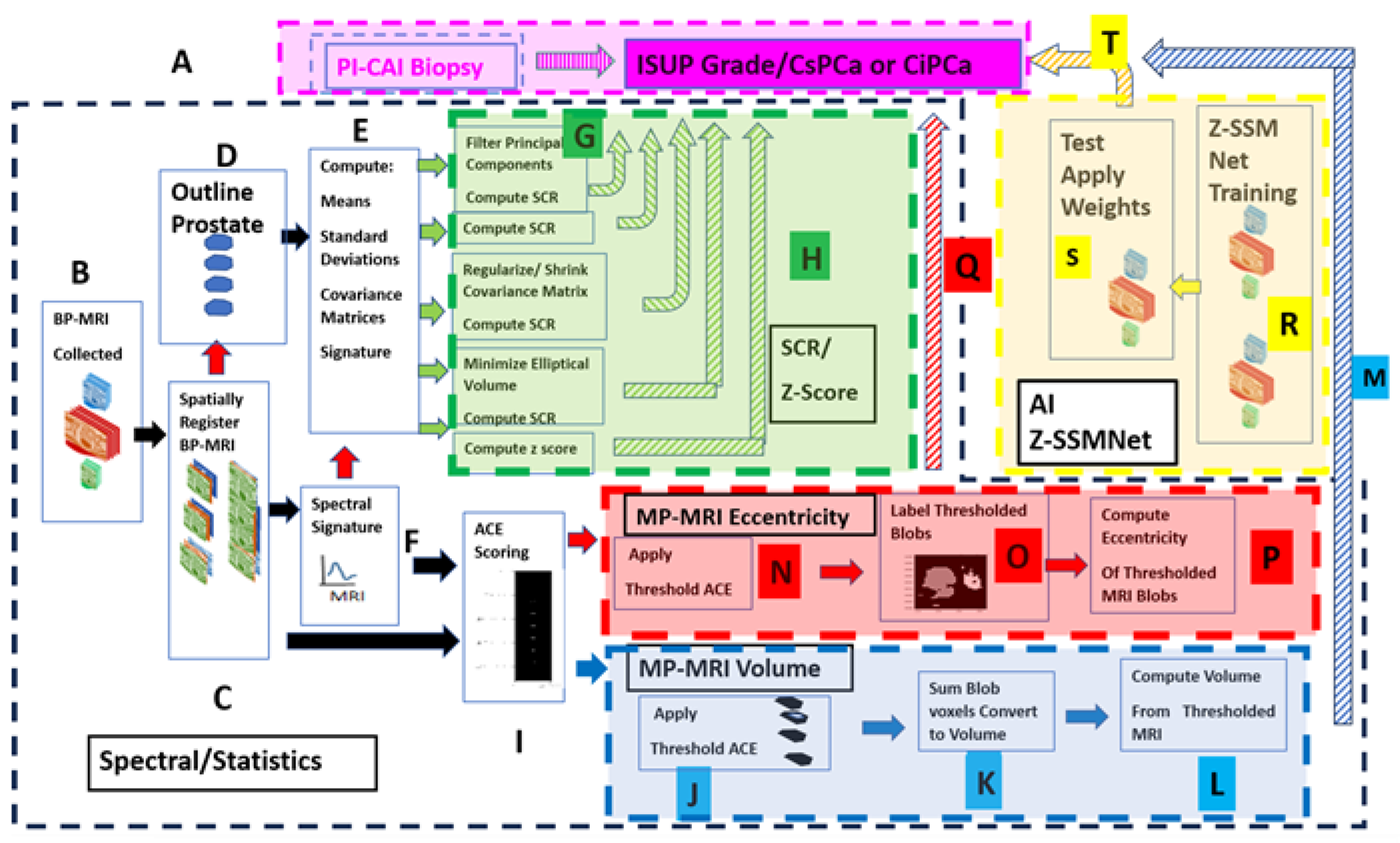
Figure 2.
Example of stitched spatially registered bi-parametric MRI, and Yuan's detection map, the color composite, and the blobbing, labeling, eccentricity and volume computations for Yuan’s detection map.
Figure 2.
Example of stitched spatially registered bi-parametric MRI, and Yuan's detection map, the color composite, and the blobbing, labeling, eccentricity and volume computations for Yuan’s detection map.
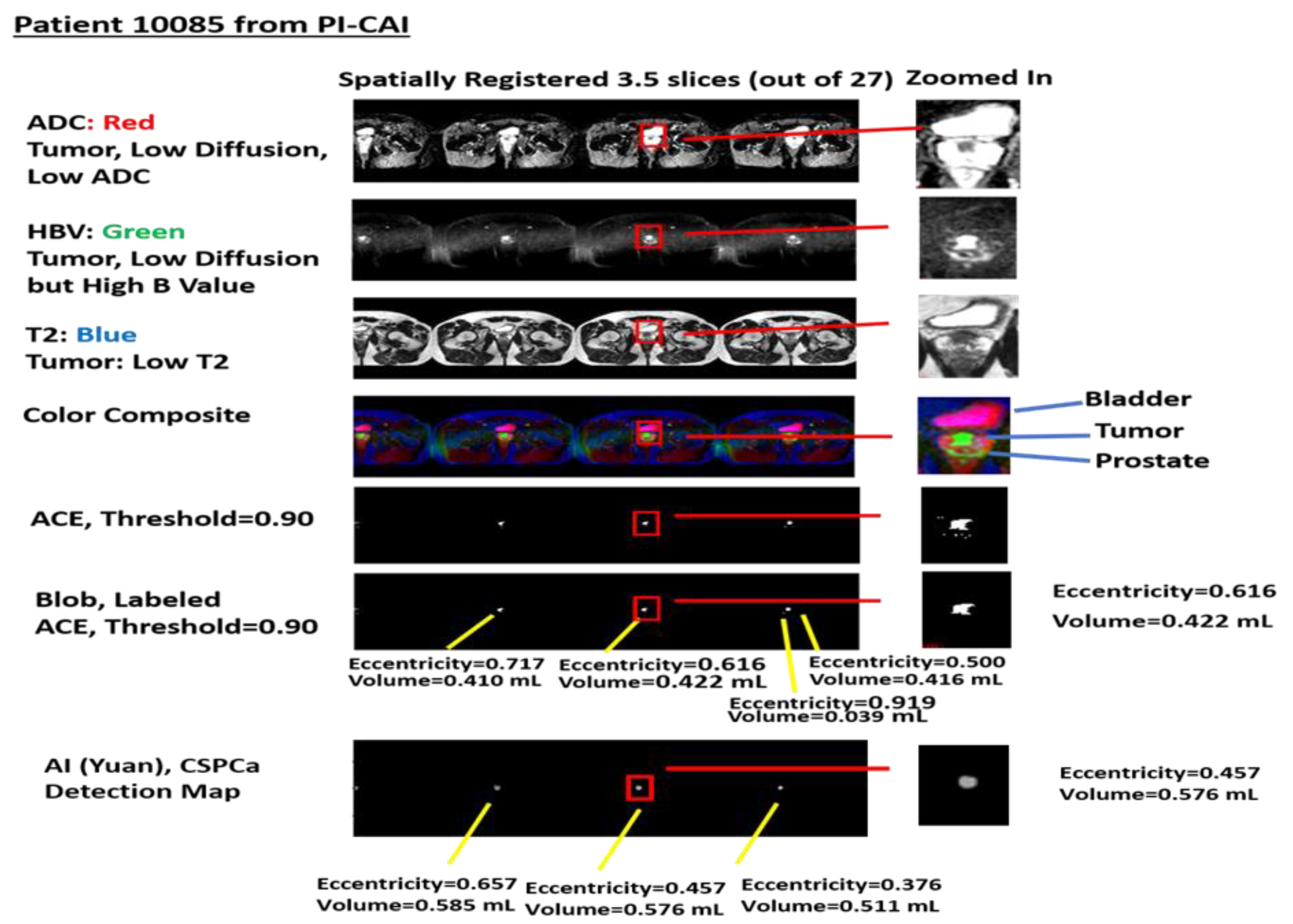
Figure 3.
Calibration plot for interpolating ISUP values from Yuan's probability of CsPCa based on linear calibration curves.
Figure 3.
Calibration plot for interpolating ISUP values from Yuan's probability of CsPCa based on linear calibration curves.
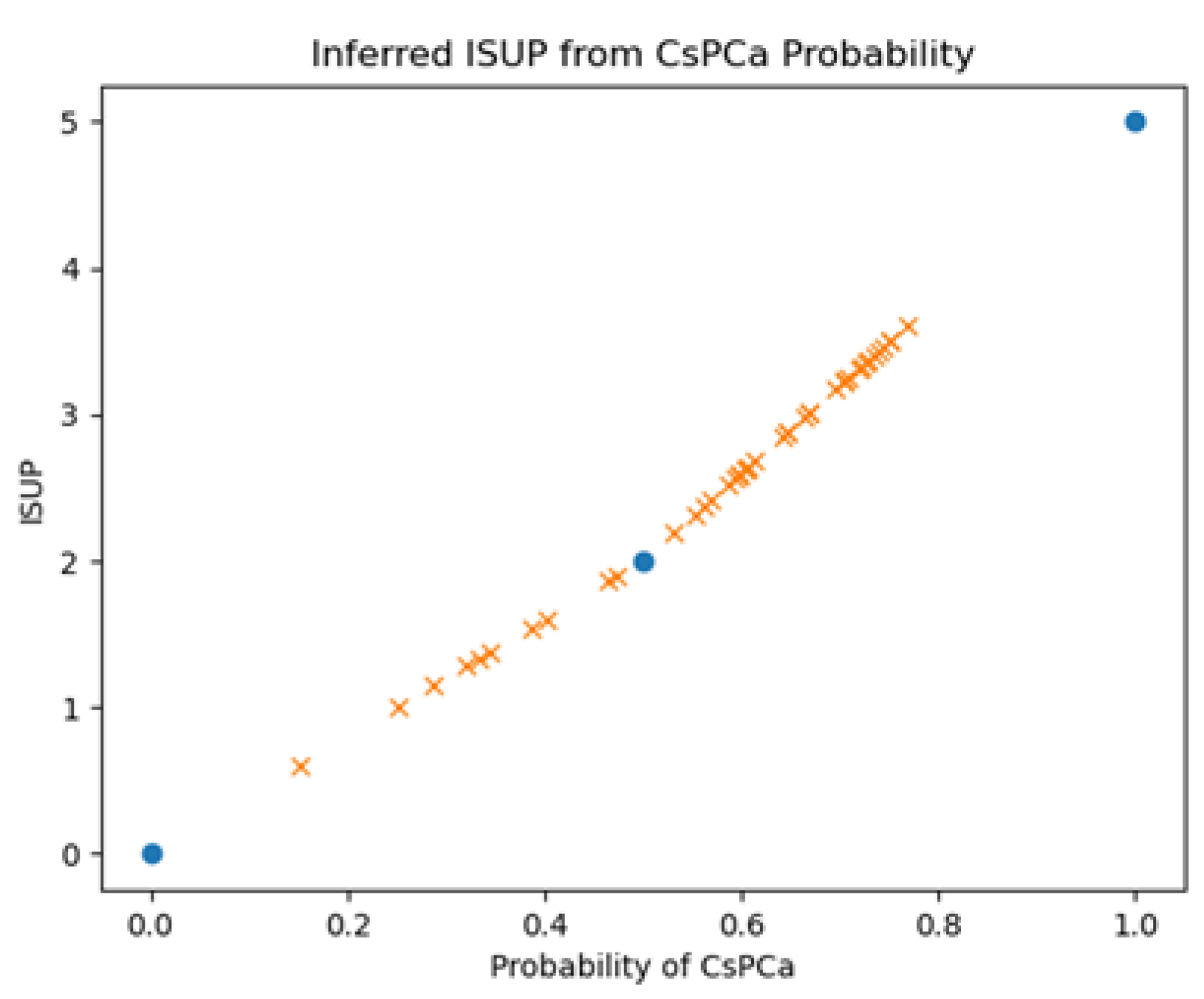
Figure 4.
Plot of features of individual patients computed from Yuan's detection map plottted against ISUP values. Correlation coefficients (R) and p-values from linear regression shown/.
Figure 4.
Plot of features of individual patients computed from Yuan's detection map plottted against ISUP values. Correlation coefficients (R) and p-values from linear regression shown/.
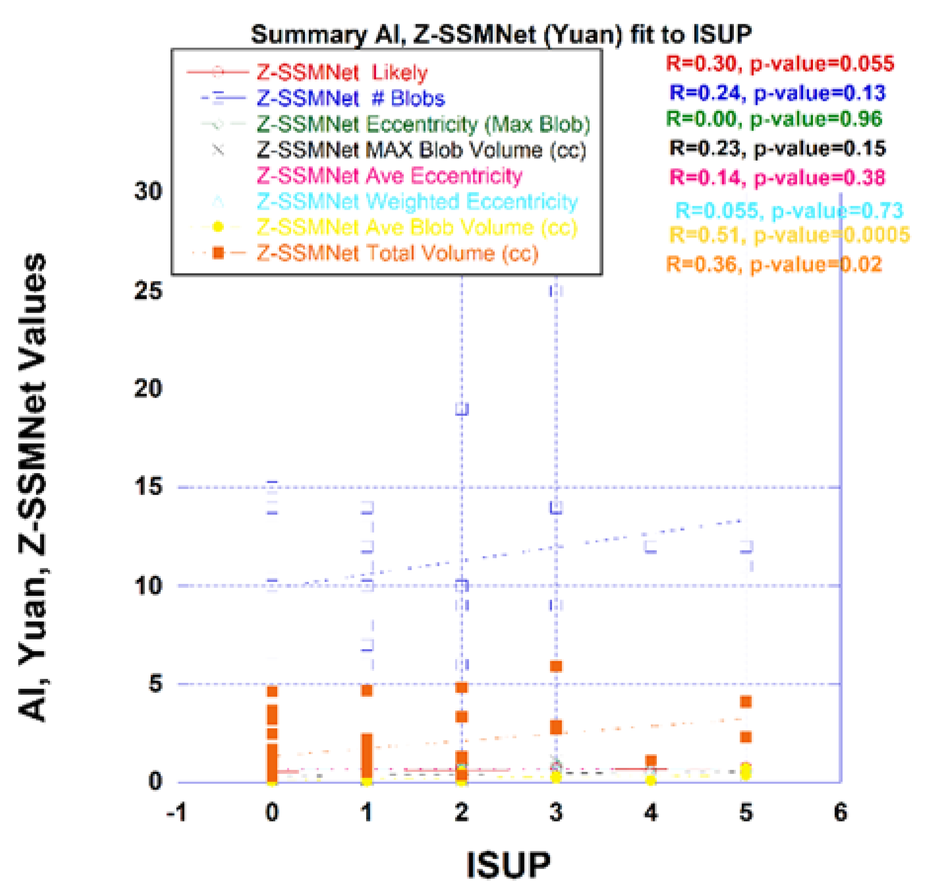
Figure 5.
Plot of multi-variate fit to ISUP combining average AI tumor blob volume and spectral/statistics SCR from modified regularization.
Figure 5.
Plot of multi-variate fit to ISUP combining average AI tumor blob volume and spectral/statistics SCR from modified regularization.
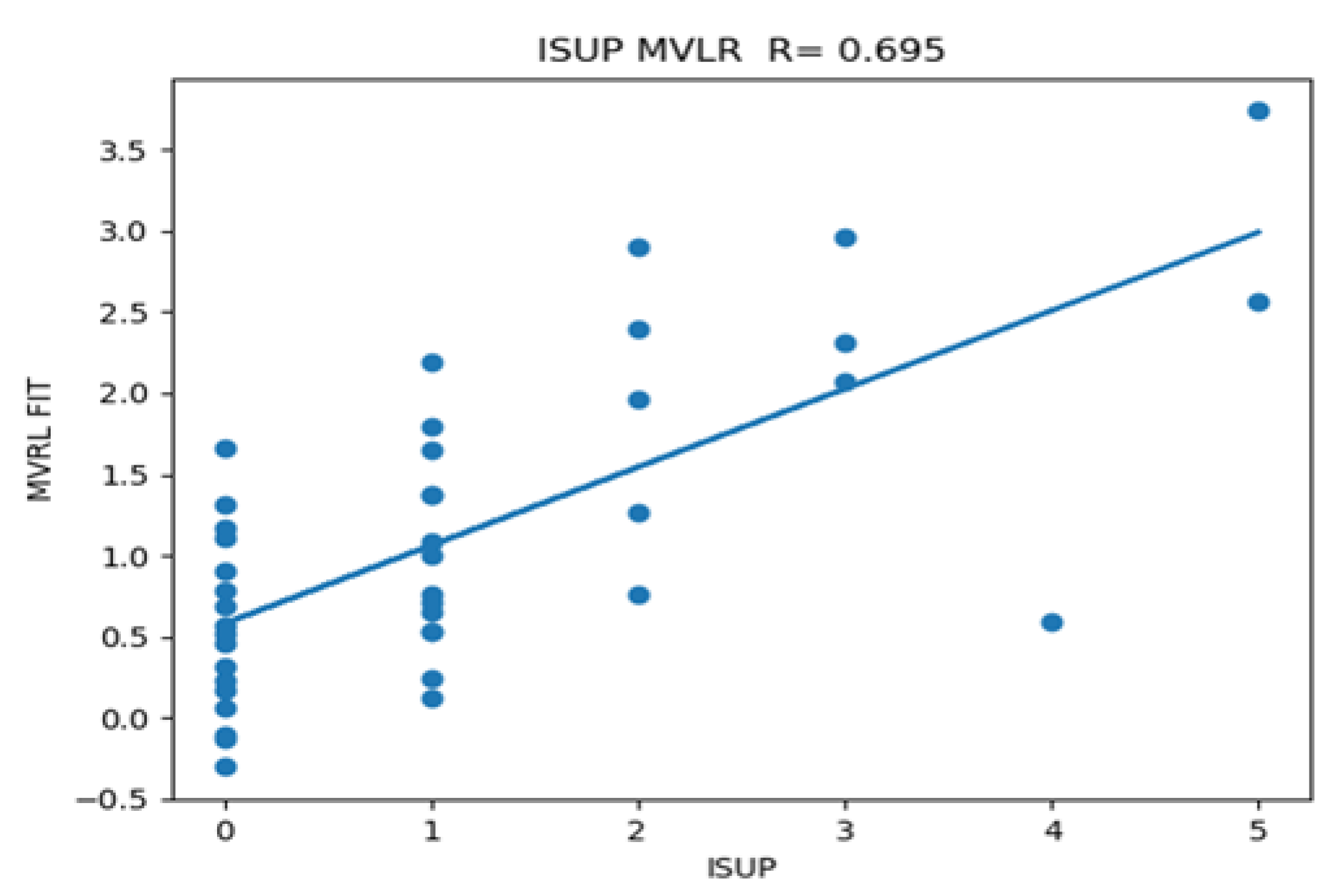

Table 1.
AI (Z-SSMNet) Linear Regression Summary.
| R | p-value | AUROC [2.5%-97.5% CI] | |
|---|---|---|---|
| Independent Variable | |||
| Probability of CsPCa | 0.298 | 0.0554 | 0.503 [0.083-1.0] |
| ISUP (Linear Conversion) | 0.301 | 0.0525 | 0.503 [0.083-1.0] |
| Average Blob Volume | 0.512 | 0.00053 | 0.367 [0.0-0.909] |
| Total Volume | 0.355 | 0.021 | 0.501 [0.0-1.0] |
Table 2.
Summary of Uni- and Multi-Variate Fit to ISUP Combining AI and Spectral/Statistical.
|
Independent Variable 1 (AI mostly) |
R1 (Uni-variate) |
Independent Variable 2 (Spectral/Statistical only) |
R2 (Uni-variate) |
Variable 1-Variable 2 Cross-Correlation |
R12 (Multi-variate) |
Probability (F-Statistic) |
|---|---|---|---|---|---|---|
| z-score | 0.532 | SCR (Modified Reg) | 0.57 | 0.985 | 0.595 | 0.0002 |
| Ave Blob Volume (AI) | 0.512 | SCR (2 PC removed) | 0.554 | 0.412 | 0.635 | 0.000042 |
| Ave Blob Volume (AI) | 0.512 | z-score | 0.532 | 0.167 | 0.683 | 0.0000059 |
| Ave Blob Volume (AI) | 0.512 | SCR (Reg) | 0.588 | 0.384 | 0.665 | 0.000012 |
| Ave Blob Volume (AI) | 0.512 | SCR (Modified Reg) | 0.57 | 0.219 | 0.695 | 0.0000026 |
Disclaimer/Publisher’s Note: The statements, opinions and data contained in all publications are solely those of the individual author(s) and contributor(s) and not of MDPI and/or the editor(s). MDPI and/or the editor(s) disclaim responsibility for any injury to people or property resulting from any ideas, methods, instructions or products referred to in the content. |
© 2025 by the authors. Licensee MDPI, Basel, Switzerland. This article is an open access article distributed under the terms and conditions of the Creative Commons Attribution (CC BY) license (http://creativecommons.org/licenses/by/4.0/).
Copyright: This open access article is published under a Creative Commons CC BY 4.0 license, which permit the free download, distribution, and reuse, provided that the author and preprint are cited in any reuse.


