Metrics of Genomic Complexity in the Evolution of Bacterial Endosymbiosis

1. Introduction

The trend towards increasing biological complexity in biological evolution is one of the most complex issues in evolutionary biology. In part, it is due to having trouble with the lack of a comprehensive definition of “biological complexity” and its measurement and universality. For instance, we can distinguish between a more complex organism than another if it has more parts, a higher hierarchical organization, or more information content in the genome [1,2,3,4]. We approach biological complexity by recurring to this last one. Assuming the genome is the information unit of living organisms and that it is a registry of the evolutionary history inherited over generations, it can give us an indication of the organism’s biological complexity [1,5,6,7,8,9].

One way to hypothetically approach the characterization of genome complexity is by resorting to some metrics that can give a general idea of the amount of information in them [5,9,10]. In this study, we use two metrics: Genomic Signature (GS) and Biobit (BB). GS is a k-mer based metric summarizing the k-mer overrepresentation regarding its expected value [9,11]. BB is a genome metric that combines the genome’s entropic and anti-entropic components, considering its k-mers entropy [9,12]. Although both metrics depend on the distribution of the frequency table of the k-mers present in the genome, they are based on different k-mer sizes and theoretical approaches making the analysis of both metrics complementary.

The evolution of endosymbiosis may be an excellent area to test whether genome complexity metrics do indeed reflect biological complexity. Endosymbiosis leads to gene loss, reduction in genome size, and increasing randomness [13,14] so it should be expected that the genomes of endosymbionts would have different metrics than the free-living bacteria from which they are evolutionarily derived. From a functional point of view, what is observed in the evolution of endosymbiosis is a systematic loss of genes until entities with minimal genomes [13,14]. The first genes to be lost from establishing the symbiotic relation are those related to mobility and some metabolic pathways for whose products the symbiont has transporters, and therefore acquires them from the host [14,15]. From this moment on, a cascade of genome reduction becomes. The process of evolution towards endosymbiosis can be an excellent area for studying the behavior of any complexity measure, including genomic complexity metrics. We expect them to yield lower values as endosymbionts become more extreme than the free-living bacteria they originate from. Previously, Moya et al. [9] used the GS and BB metrics in cyanobacterial genomes, concluding that both metrics could measure complexity. However, there was a lack of understanding of these measures in a regressive event. The present study tests whether GS and BB metrics change their values in bacterial endosymbionts to free-living bacteria, supporting the hypothesis of metrics of genome complexity.

2. Materials and Methods

2.1. Genomes Set and Species Phylogeny

We selected 80 fully sequenced genomes from endosymbiont organisms of three bacterial clades: Bacteroidota, Oceanospirillales, and Enterobacterales. To compare them and assess the trend to the endosymbiosis analyses, we added 72 free-living bacteria to root each of these clades of endosymbionts. We differentiate both lifestyles with the keyword Habitat. The 20 endosymbiont Bacteroidetes were rooted with 20 free-living Cytophagales species, 15 endosymbionts of Oceanospirillales species were rooted with 15 free-living species from the same clade, and, finally, we rooted the 45 Enterobacterales with 37 free-living Alteromonadales. In this last case, we used fewer free-living species due to the sequencing bias to pathogens and parasites and the assembly quality. 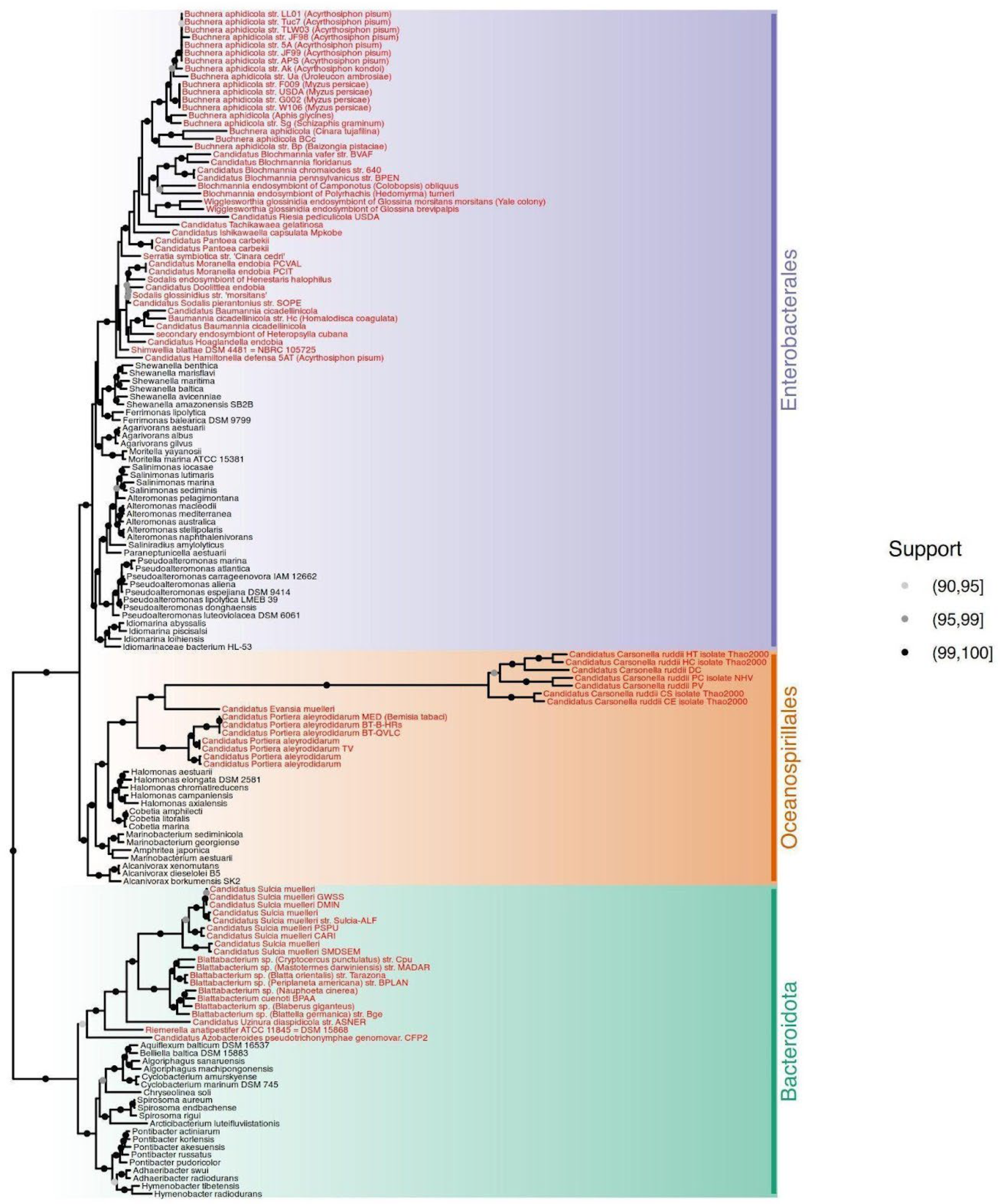To root the tree, we used seven Fusobacteria species (Table S1 and Table S2). Maximum Likelihood phylogenetic trees using a concatenated alignment of 16S and 23S rRNA genes (3,981 positions) and 27 conserved proteins (alignment supermatrix with 4102 positions) are shown in Figure S1 and Figure 1. The rRNA tree scored a mean support of 95.04% based on ultrafast bootstrap with 4,000 replicates [16], whereas the 27 ribosomal proteins supermatrix tree scored a 95.44% mean support.

We reconstructed two trees: from a 16S and 23S rRNA sequences supermatrix and a set of 27 conserved protein domains supermatrix. The rRNAs were retrieved directly from the genomes set using barrnap v0.9 (https://github.com/tseemann/barrnap). Barrnap did not detect sequences and one 23S sequence, and we manually extracted it from the annotation files. For the GTDB proteins set [17], we downloaded the alignment profiles from PFAM and performed an HMM search [18] over all the protein sets of the study genomes. Finally, we got those proteins with coverage higher than 75% and more than 150 species and removed the possible paralogous sequences (Table S3). We independently aligned the three rRNAs and conserved protein domain sequences using MAFFT-L-INS-i v7.490 [19]. Then, we trimmed the aligned sequences with trimAl v1.4.15 [20] using the gappyout option. Once aligned and trimmed, the sequences of each set (rRNAs and protein domains) were concatenated, and they were used to infer the species tree. Phylogenies were inferred using IQ-TREE v2.1.3 [21], and the model was selected using ModelFinder [22]. We restricted the models to two sets: JC, HKY, K2P, GTR, SYM for the rRNAs concatenated alignment, and WAG, JTT, LG, and JTTDCMut for the conserved proteins concatenated alignment. The robustness of the trees was assessed with 4,000 ultrafast bootstrap replicates [16].

2.2. Genomic Metrics and Parameters Calculation

For each genome, we computed two genome metrics: GS and BB (see the next sections for details). We also retrieved six genomic parameters from the GFF (annotation file that describes DNA, RNA, and protein sequences) files linked to each genome (number of CDS, number of genes, number of rRNAs, gene mean length, genome length, and GC content) and added the percentage of hapaxes. A hapax is defined as a sequence appearing just once in a genome, or in this case, a k-mer with an absolute frequency of 1 in the frequency table of the k-mers of a genome, for a given value of k. We computed the percentage of hapaxes to the total number of k-mers.

2.3. Genome Signature (GS)

The GS metric focuses on the k-mers content of a given genome [9]. For an alphabet of four characters, as DNA, and defining a word length of k characters, we can obtain a maximum of 4^k words (k-mers). Then, the expected occurrence value of every k-mer is

$$EV=\left({\sum }_{j=1}^{4^k}{n}_j/4^k\right),$$

where $n_j$ is the total number of k-mers found in the genome. For a specific value of k, a value of GS (GS_k) can be calculated as

$${GS}_k={\displaystyle \frac{1}{\sum _{j=1}^{4^k}n}}·\sum _{i=1}^{4^k}\left|n_i-EV\right|.$$

$n_i-EV$ serves as mean centering, with $n_i$ being the number of k-mers found for a specific sequence, and the final value is divided by

$$\sum _{j=1}^{4^k}{n}_j,$$

so that comparison between genomes of different sizes can be made. To obtain the optimum value of k for a given genome, first a random genome with the same size and the same base composition as the given genome is created. Then, GS_k is calculated on the provided genome (GS_g) and the random genome (GS_r), starting from k = 2 and GS_r is subtracted from GS_g, to remove random noise from the metric, to obtain a preliminary value of GS (GS_p).

$${GS}_p={GS}_g-{GS}_r.$$

Finally, we repeat the procedure increasing the value of k up to 16_.The GS value for that genome is the maximum value obtained for GS_p.

2.4. Biobit (BB)

The BB metric is a logistic map that balances a genome’s entropic and anti-entropic components [12]. BB compares the true genome with a random equifrequent one with the same length. First, the k-mers yielding maximum entropy of real and random equifrequent genomes are calculated and compared. The entropy of a genome of length G (E_2L(G)) takes a value between the minimum (log₄(G), denoted L(G)) and the maximum (2L(G)). They also calculate the entropic (E(G) = E_2L(G) – L(G)) and anti-entropic (A(G) = 2L(G) – E_2L(G)) components of the genome. Then E(G) + A(G) = L(G). These elements can be combined, nonlinearly, by

$$BB\left(G\right)=\sqrt{L\left(G\right)}\sqrt{{\displaystyle \frac{A\left(G\right)}{L\left(G\right)}}}{\left(1-2{\displaystyle \frac{A\left(G\right)}{L\left(G\right)}}\right)}^3.$$

2.5. Statistical Analyses

We performed a correlation analysis between all the genomic variables and the complexity indexes retrieved. The reason behind this analysis is to assess what variables may be affecting each of the metric values and to evaluate if any of the metrics indicate functionality. Phylogenetically informed correlations were done using an in-house function with the variance-covariance matrix, calculating Pagel’s lambda [23,24] for each pair of traits calculated using the phytools v2.1-1 [25] R package. This matrix was converted to correlations between traits matrix with stats R package (https://www.r-project.org/). Finally, t values for each correlation value r were obtained by $t=r\sqrt{(n-2)/(1-r^2)}$, and a p-value derived from a t-student distribution with n – 2 degrees of freedom. The p-values were corrected by the Holm-Bonferroni method [26] to control the family-wise error rate (FWER).

We used two-sample comparisons to contrast the differences between free-living and endosymbiont organisms in each variable. We applied phylANOVA [23], to take into account the phylogenetic relationships among lineages. The same dataset has also been used to assess a principal component analysis (PCA) to investigate further the effect and relationship of the genomics variables on, and between, the complexity indexes and to assess which variables better characterize the differences between the samples. We used the correlation matrix to do the PCA, as the scales of the variables were very different. The PCA was phylogenetically informed by in-house functions using phytools, calculating Pagel’s lambda for the whole matrix [23,24].

2.6. Phylogenetic Signal

Pagel’s lambda was used to inform correlations and PCAs phylogenetically. The phylogenetic signal of each trait in the entire tree and the three clades was analyzed using Blomberg’s K [27]. When K is significantly different from zero, the trait shows a phylogenetic signal; that is, the trait resembles more in closer species than expected by chance. A robust phylogenetic signal is assumed when K > 1 since K = 1 is the predicted value under Brownian evolution.

3. Results and Discussion

3.1. Phylogenetic Analyses

To analyze the endosymbiosis phylogenetic transition, we first selected 152 bacterial genomes, 80 of which are from bacterial endosymbionts and the other 72 from free-living bacteria (Tables S1 and S2). These free-living bacteria draw the evolutionary path to endosymbiosis in three main lineages: Bacteroidota phylum, Enterobacterales, and Oceanospirillales orders. We used seven Fusobacteria species to root the entire tree. As indicated, the transition to endosymbiosis was assessed using free-living relatives for each lineage. As expected, the Oceanospirillales and Enterobacterales form a sister clade of the Bacteroidota. The internal topology of each group differs between rRNA and protein trees. In the case of the rRNA tree (Figure S1), some free-living Oceanospirillales are in the root of Proteobacteria, and others are placed in the root of the Alteromonadales and Enterobacterales clade. Despite this topology, the protein supermatrix tree (Figure 1) resolves these arrangements better, and the three groups are correctly clustered, following previously reported topologies [17,28]. Thus, the protein supermatrix tree was used for the analysis where a tree was needed.

3.2. Phylogenetic Signal

Almost all phylogenetic signals of all the study traits across the whole tree and in the three clades where endosymbiotic events occurred (Figure S2 and Table S4) were significant. None of the phylogenetic signals were stronger than Brownian evolution (i.e., K > 1) in the whole tree or the Enterobacterales clade. However, some traits with K > 1 were found in the Oceanospirillales (number of genes and CDS, genome length, and GC content) and Bacteroidota (GC content and GS) clades. 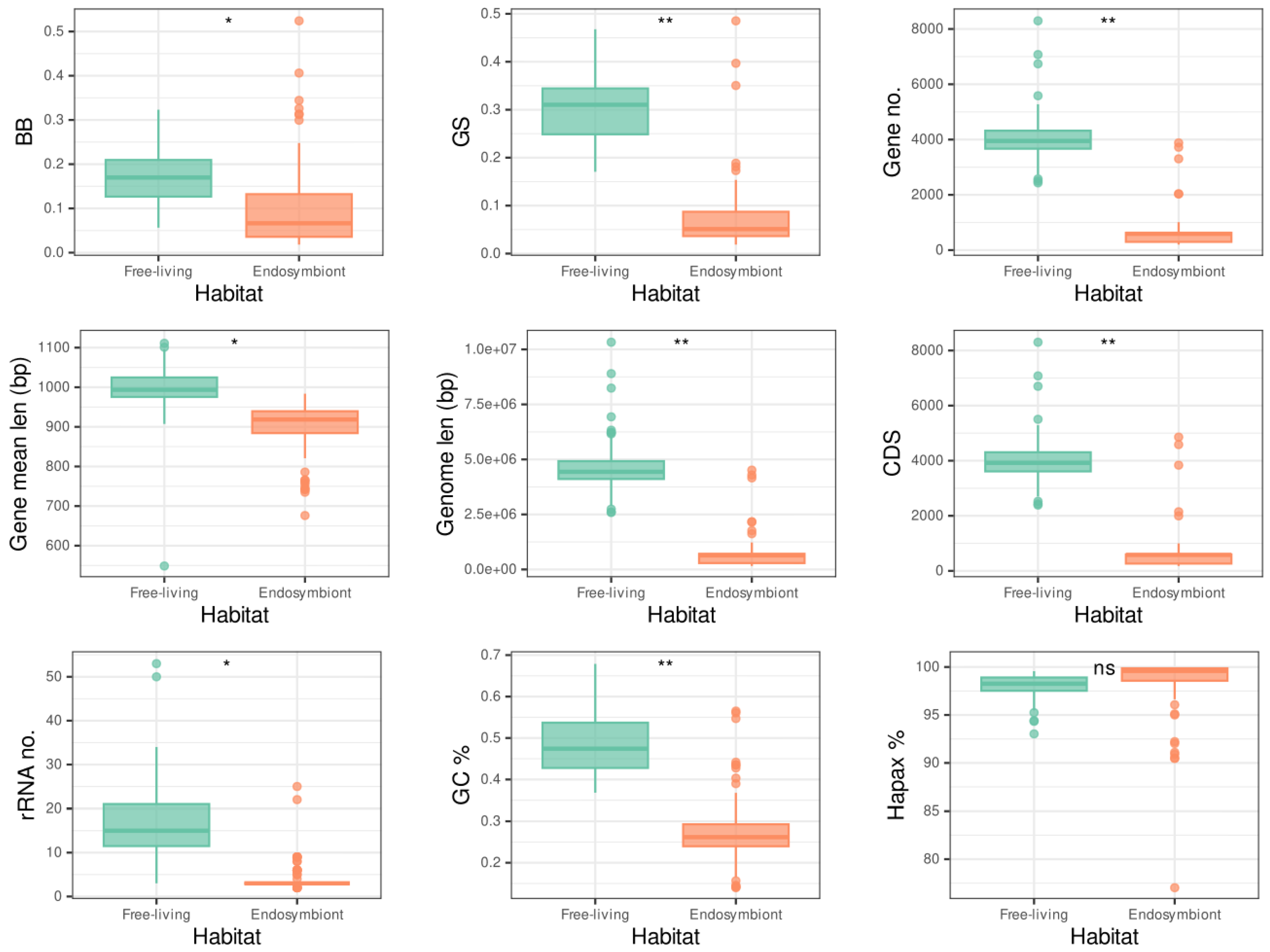Taking Brownian motion as a reference, K values greater than 1 indicate more variance among clades than expected by chance. In contrast, values lower than 1 indicate more variance within clades than expected by chance. When studying the differences in distribution for many of the traits between endosymbionts and free-living organisms (Figure 2), the greater differences seem to correlate with greater values of K, which would make sense as the difference among the clades is greater than expected.

3.3. Metrics, Genome Parameters, and Phylogenetic Correlations

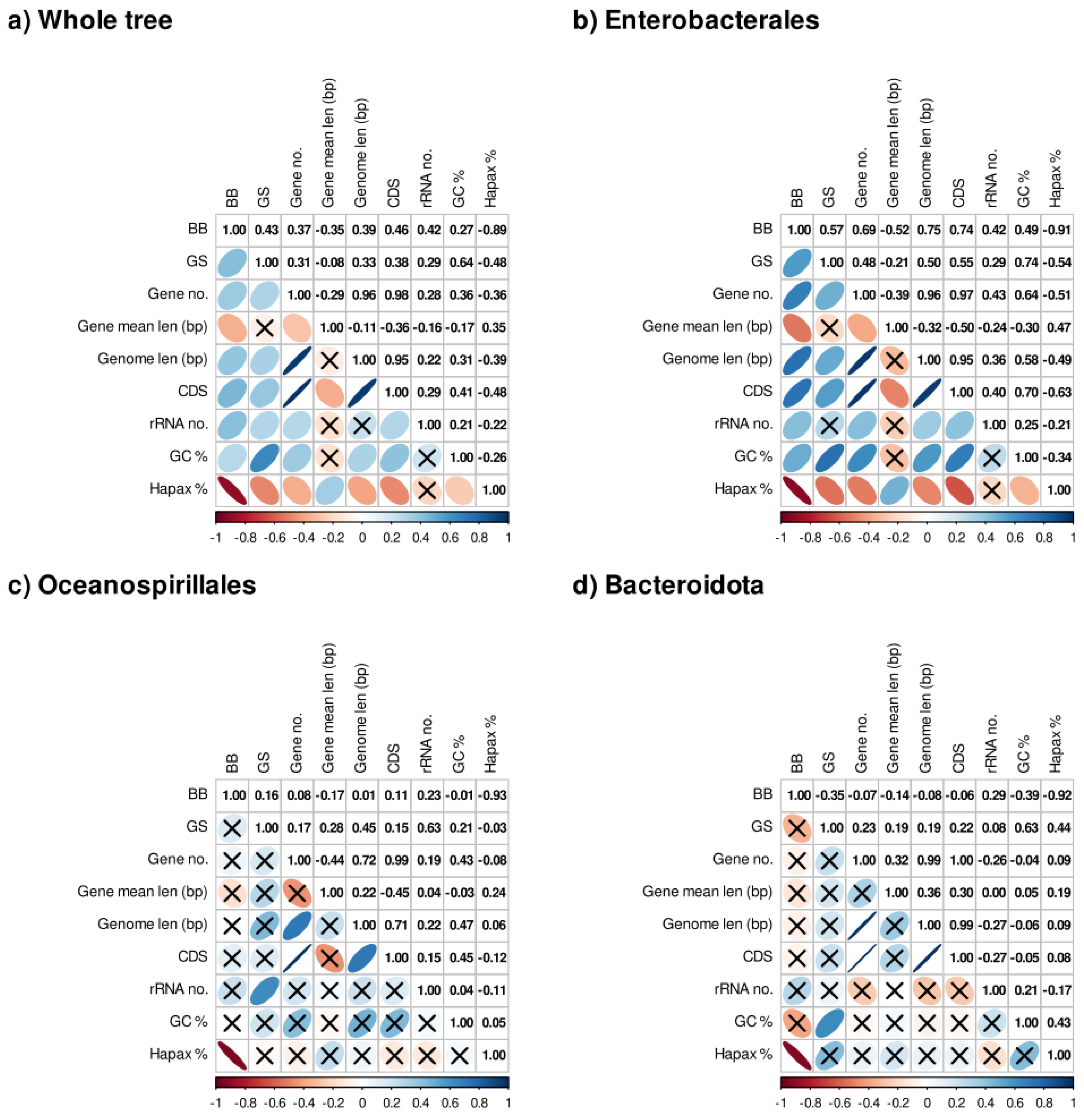
Table S5 shows the values of the metrics and parameters calculated (from now on, traits when referring to both). To assess if both metrics indicate functionality, we carried out phylogenetic correlation analyses concerning the genome parameters for the whole tree and the three lineages, respectively (Figure 3). As can be observed, GS and GC content show a moderate positive (0.64) relationship in the entire tree (Figure 3a), in the Bacteroidota clade (0.63) (Figure 3d) and turns stronger in the Enterobacterales clade (0.74) (Figure 3b). In the case of BB, the only correlation with an absolute coefficient greater than 0.85 is with the percentages of hapaxes, which holds in every lineage. Nevertheless, in the case of the Bacteroidota and Oceanospirillales (Figure 3c and 3d), many correlations were not statistically significant, possibly due to the lower number of taxa involved.

3.4. Principal Component Analysis of Traits Discriminates Between Bacteria Lifestyles

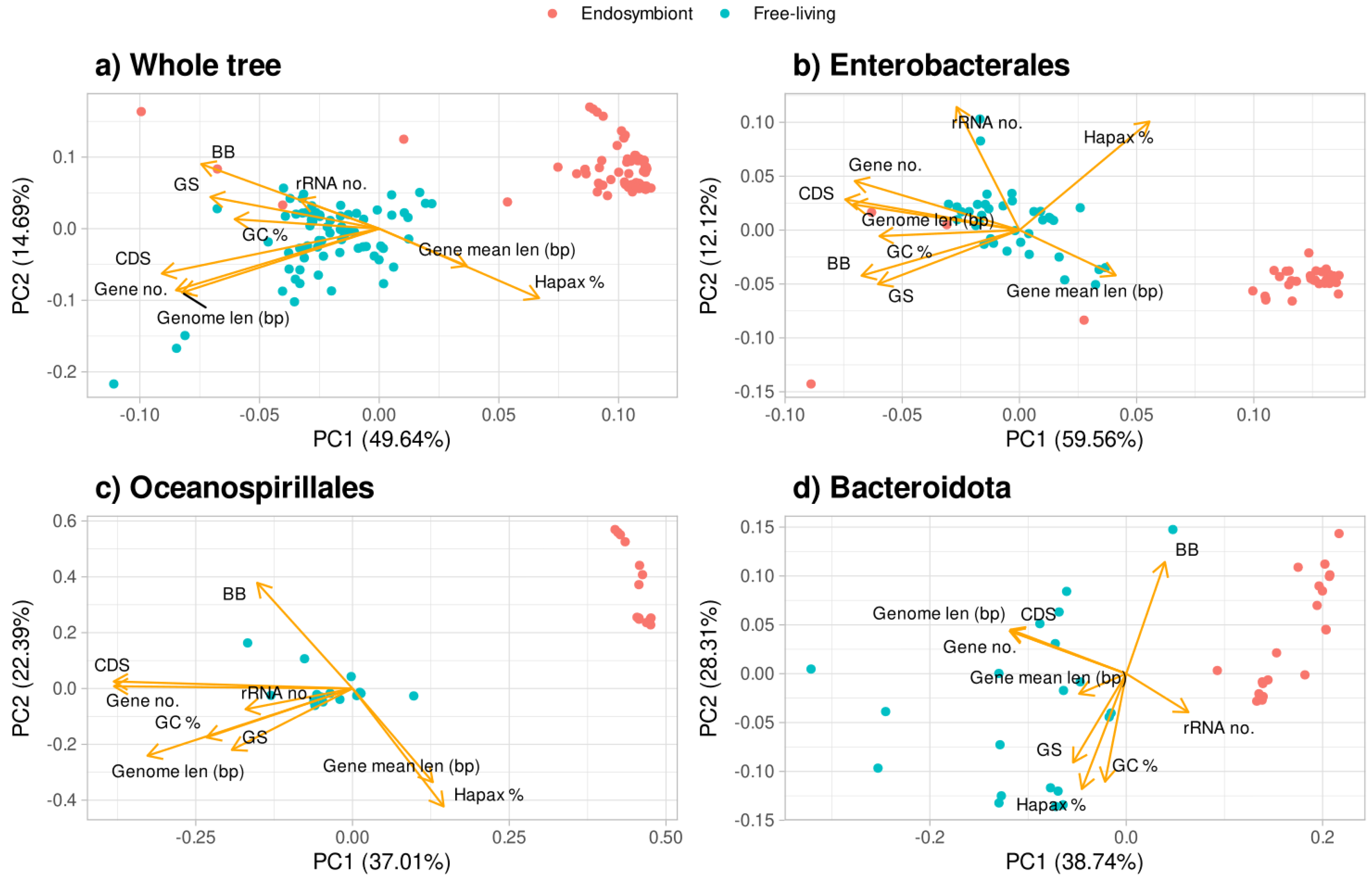
The principal component analysis (PCA) of all the traits (metrics and parameters) reveals that these traits discriminate between the habitats of the organisms (Figure 4). For all bacteria studied (Figure 4a), the first component is almost capable of distinguishing between free-living and endosymbiont organisms on its own. For the calculation of this component, the more important variables are the number of CDS, number of genes, genome length, and percentage of hapaxes. In the case of the Enterobacterales lineage (Figure 4b), three clusters are observed, with the free-living organisms being the ones in the center. When analyzing the Oceanospirillales and Bacteroidota lineages, the first component is enough to discriminate between the lifestyles (Figure 4c and 4d).

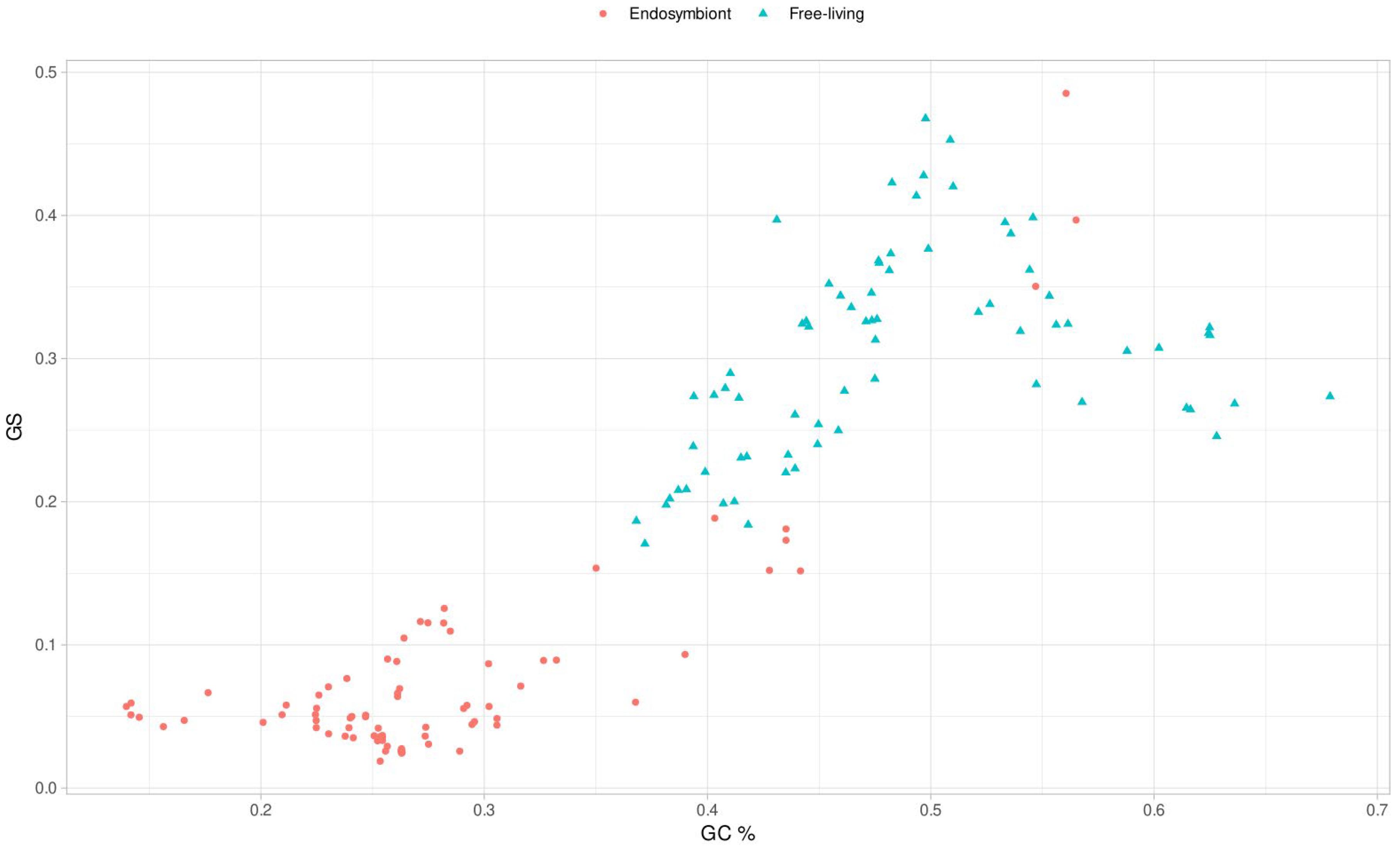
3.5. Genomic Base Composition Drives the GS and BB Values

Analyzing the results of the phylogenetic correlations in depth, in the case of the analysis of the GC content versus the value of GS, we obtained a moderate positive relationship in most of the clades. To analyze this in detail, we represented the correlation for all the genomes (Figure 5). As can be observed, there is a quadratic correlation pattern where the maximum value of GS corresponds to the genomes with a GC content near 50%. When the values of GC content decrease or grow around 50%, the GS metric values always tend to decrease. This decrease in the GS metric with extreme GC content values indicates that the metric may be related to the randomness of the genome sequence, as a genome with equiprobable base frequencies is more likely to have an even distribution of k-mers. A genome with uniform base frequencies would lead to a more random genome (maximum GS) than one with a biased nucleotide bases composition, where the probability of specific arrangements of nucleotide bases of length k would be higher.

GS is a measure based on the overrepresentation and underrepresentation of the k-mers. Thus, more homogeneous genomes with a high amount of a pair of nucleotide bases, such as A and T in the case of endosymbionts, will favor the overrepresentation of AT-rich k-mers, which will result in an uneven distribution of the k-mer frequency and, thus, in higher $n_i$ values. Consequently, $n_i$>> EV produces an increase in GS_g (see the GS equation in methods). Otherwise, genomes with equal proportions of nucleotide bases (GC content around 50%) will provide an even k-mers distribution, resulting in $n_i$ values closer to their EV, approximating the term $\left|n_i-EV\right|$ to 0, leading to lower GS_g values. Then, why is the opposite behavior observed in Figure 5? It is due to the effect of GS_r in the calculation of the metric. In the genomes of the endosymbionts there is an overrepresentation of AT-rich k-mers and considering that with GS we are working with k values relatively small, that makes the frequency tables of the given genome and the random genome quite similar in distribution. The values of GS_g and GS_r are far more similar the further away the given genome is from a 50% GC content. The representation of GS_r and GS_g against GC content is shown in Figure S3, supporting the presented idea. We see this mathematical reasoning in the data where we can observe the peak in Figure 5 occurring strictly at a GC content of 50%. Then, uneven k-mer distributions due to GC content decrease the GS value. This peak is the reason behind the linear correlation values between both traits. However, as seen here, they are closely related. When we computed a quadratic regression with the data, we obtained a multiple R-squared of 0.7733 with an adjusted R-squared of 0.7703, showing a high quadratic correlation.

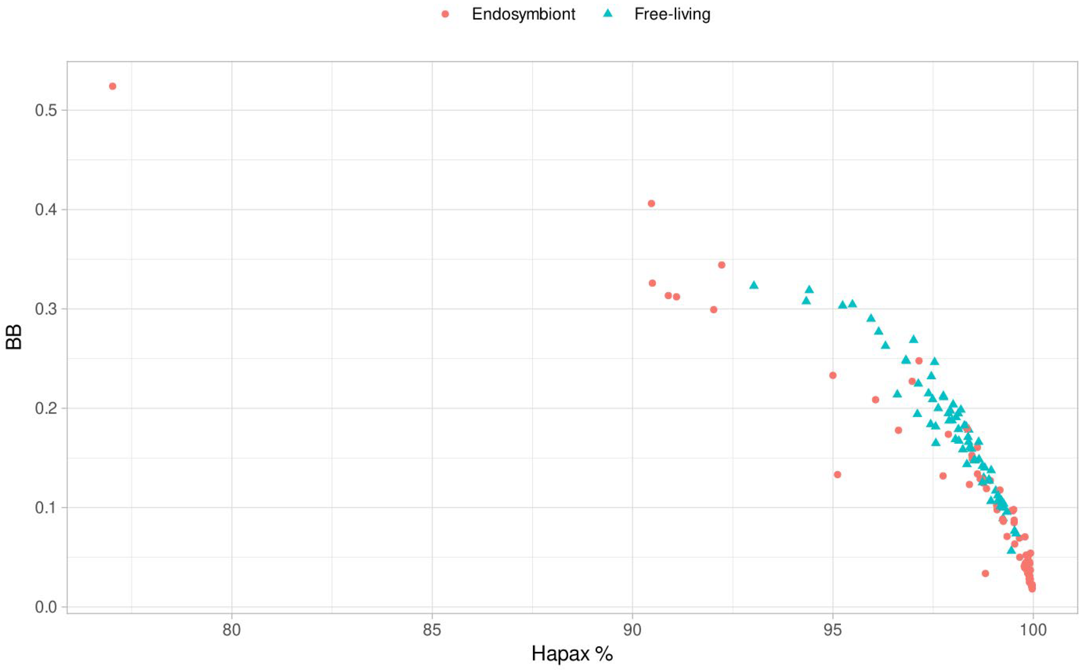
We also observed that the percentage of hapaxes is strongly positively correlated in all the clades. When analyzing BB, we then represented the percentage of hapaxes versus the value of BB to observe how these unique k-mers’ presence may be driving the metric (Figure 6). We can observe a significant negative Pearson correlation of -0.89, so the percentage of hapaxes may influence the metric so that the higher the number of k-mers appearing once, the lower the metric value. That is also consistent with the metric principles because, in random genomes, all k-mers should be hapaxes [12]. We also observed seven endosymbiont outliers in the BB metric (Figure 2), allowing us to analyze these organisms’ nature and metrics further. It is worth noticing that these outliers tend to present higher or similar values to the free-living bacteria with the highest BB. But why is BB so higher in the outliers?

3.6. Outlier Analyses of BB

The higher value of BB corresponds to Candidatus Sodalis pierantonius str. SOPE, a Sitophilus oryzae primary endosymbiont [29]. The genome of this organism presents a high percentage of mobile elements, especially insertion sequences (IS), typically present at the first stages of the endosymbiont process, as is the case of this endosymbiont. The high percentage of these repetitive mobile elements decreases the percentage of hapaxes, favoring the homogeneity of the genome, and seems to increase the value of BB.

The following higher value of BB corresponds to Candidatus Hamiltonella defensa 5AT, a secondary endosymbiont of Acyrthosiphon pisum [30]. This genome is also colonized by mobile elements that constitute around 20% of the genome, leading to a decrease in the percentage of hapaxes and an increase in the metric.

The next organism with a high BB value is Sodalis glossinidius str. ’Morsitans’ a secondary endosymbiont of Glossina morsitans [31]. In this case, a moderate percentage of IS (around 2.5% of the genome) was observed, possibly linked to a recent evolutionary link between the endosymbiont and the host [32]. The presence of these sequences decreases the percentage of hapaxes as before, increasing the metric value. In these three previous examples, we observed some of the highest percentages of GC in our endosymbiont dataset (more than 40%) and are also some of the largest endosymbiont genomes in our dataset, possibly indicating a recent evolutionary link with their respective hosts.

Finally, the last four outliers correspond to the same organism, Candidatus Carsonella ruddii, a primary endosymbiont of different species of psyllids [33]. Unlike what we observed with C.H. defensa and S. glossinidius, these organisms have the lower percentages of GC in our endosymbiont dataset (around 15%) and are the shorter ones of that dataset (less than 160.000 bases). The percentage of hapaxes is lower because this genome seems to keep some specific sequences, leading to the retention of some specific k-mers, which decreases the total percentage of hapaxes due to the short size of the genomes. This decrement, as before, seems to increase the value of BB.

As can be seen, the number of hapaxes is inversely related to BB. Moreover, the hapaxes proportion is directly related to the genome heterogeneity; the lower the number of hapaxes, the higher the homogeneity of a genome (as it has more repeated k-mers). Conversely, a genome with a high proportion of hapaxes turns more heterogeneous as less repetitive k-mers are seen. Thus, we could relate BB to the k-mer heterogeneity.

3.7. Genome Complexity and Metrics

To assess the complexity hypothesis, we first studied the statistical difference of each metric between the free-living and endosymbiont lifestyles for each group, informing the tests with the corresponding phylogeny. Some genomic parameters show significantly lower values for the endosymbiont genomes in some of the lineages (Figure S4 and Table S6). These are number of genes in all the lineages, genome length and CDS in Enterobacterales and Oceanospirillales, and GC content in Oceanospirillales. With GS a significant difference can be observed in the whole tree and in the Oceanospirillales, while BB shows no significantly lower values for the endosymbionts in any clade. This non-significant difference in the case of the Enterobacterales is due to the presence of the outliers mentioned above, which manifest as outliers in all the whole tree and Enterobacterales plots. If we remove the seven outliers, there is a significant difference in the BB values between the endosymbionts and the free-living organisms in the whole tree (p-value 0.042) but noy in the Enterobacterales (p-value 0.12). In the case of GS removing these outliers reveal keeps the significant difference in the whole tree (p-value 0.009) and there is also a significant difference in the Enterobacterales (p-value 0.03). Notwithstanding, instead of perceiving the same behavior, BB and GS do not show remarkably significant differences between endosymbionts and free-living organisms in Bacteroidota, and only GS is able to discriminate the two habitats in the case of the Oceanospirillales. In the case of BB it may be due to having fewer taxa in those two clades than in the Enterobacterales one. GS ability to discriminate in the case of the Oceanospirillales may be explained by analyzing the base composition of the genomes (Figure S5). As can be seen when the difference in the AT content (or GC content) is greater between the habitats the metric seems to discriminate better between them. With the results obtained, GS represents a complexity that is more based on the informational content of the genomes and its relationship with entropy. In contrast, BB represents a complexity based on the measure of the adaptability or plasticity of the genome, as observed in the case of its outliers in transitional phases of the endosymbiosis process which are supposed to have been more subjected to a higher dynamism.

In the case of GS, the degeneration process characteristic of the endosymbionts brings the genomes to a base composition that deviates more from a 50 % GC content, thus decreasing the metric. With BB, free-living organisms tend to have a greater value of the metric, which correlates with the theoretical biological complexity. Still, we observe a higher value of BB on the genomes of species in a transitional stage due to the content of repetitive structures.

4. Conclusions

We show that GS decreased during the endosymbiosis process, and BB has significant differences in one of the clades and the whole tree if we factor the outliers out. In the case of BB, we explained the Enterobacterales outliers within the context of the first steps of the endosymbiosis process.

We also observed that the selection towards AT in endosymbiont genomes is related to lower values of GS. This metric accounts for the representation of the k-mers by retrieving their frequency to the expected number of k-mers to find. Thus, more homogeneous genomes have more similar k-mers, an overrepresentation of certain k-mers. Taking into account the behavior of the metric when analyzing the random genome, the lower values in the case of the endosymbionts are explained.

We concluded that GS may be too limited to the actual contents of the genome and their relationship with the entropy of a random genome. At the same time, BB shows more promise as a metric that could quantify a larger part of the complexity of the genome and its adaptability.

References

- Adami, C. What Is Complexity? Bioessays 2002, 24 (12), 1085–1094. [CrossRef]
- McShea, D. W.; Brandon, R. N. Biology’s First Law: The Tendency for Diversity and Complexity to Increase in Evolutionary Systems, 1st ed.; University of Chicago Press: Chicago, IL, USA, 2010.
- Koonin, E. V. The Meaning of Biological Information. Philosophical Transactions of the Royal Society A: Mathematical, Physical and Engineering Sciences 2016, 374 (2063). [CrossRef]
- Heim, N. A.; Payne, J. L.; Finnegan, S.; Knope, M. L.; Kowalewski, M.; Lyons, S. K.; McShea, D. W.; Novack-Gottshall, P. M.; Smith, F. A.; Wang, S. C. Hierarchical Complexity and the Size Limits of Life. Proceedings of the Royal Society B: Biological Sciences 2017, 284 (1857). [CrossRef]
- Adami, C.; Cerf, N. J.; Kellogg, W. K. Physical Complexity of Symbolic Sequences. Physica D 2000, 137.
- Adami, C.; Ofria, C.; Collier, T. C. Evolution of Biological Complexity. Proc Natl Acad Sci U S A 2000, 97 (9), 4463–4468. [CrossRef]
- Adami, C. What Is Information? Philosophical Transactions of the Royal Society A: Mathematical, Physical and Engineering Sciences 2016, 374 (2063). [CrossRef]
- Moya, A. The Calculus of Life, 1st ed.; SpringerBriefs in Biology; Springer International Publishing: Cham, Switzerland, 2015. [CrossRef]
- Moya, A.; Oliver, J. L.; Verdú, M.; Delaye, L.; Arnau, V.; Bernaola-Galván, P.; de la Fuente, R.; Díaz, W.; Gómez-Martín, C.; González, F. M.; et al. Driven Progressive Evolution of Genome Sequence Complexity in Cyanobacteria. Scientific Reports 2020 10:1 2020, 10 (1), 1–14. [CrossRef]
- Adami, Christoph. The Evolution of Biological Information : How Evolution Creates Complexity, from Viruses to Brains, 1st ed.; Princeton University Press: Princeton, NJ, USA, 2024.
- de la Fuente, R.; Díaz-Villanueva, W.; Arnau, V.; Moya, A. Genomic Signature in Evolutionary Biology: A Review. Biology 2023, Vol. 12, Page 322 2023, 12 (2), 322. [CrossRef]
- Bonnici, V.; Manca, V. Informational Laws of Genome Structures. Scientific Reports 2016 6:1 2016, 6 (1), 1–10. [CrossRef]
- Delaye, L.; Moya, A. Evolution of Reduced Prokaryotic Genomes and the Minimal Cell Concept: Variations on a Theme. BioEssays 2010, 32 (4), 281–287. [CrossRef]
- Moran, N. A.; Bennett, G. M. The Tiniest Tiny Genomes. Annu Rev Microbiol 2014, 68 (Volume 68, 2014), 195–215. [CrossRef]
- Husnik, F.; Tashyreva, D.; Boscaro, V.; George, E. E.; Lukeš, J.; Keeling, P. J. Bacterial and Archaeal Symbioses with Protists. Current Biology 2021, 31 (13), R862–R877. [CrossRef]
- Hoang, D. T.; Chernomor, O.; Von Haeseler, A.; Minh, B. Q.; Vinh, L. S. UFBoot2: Improving the Ultrafast Bootstrap Approximation. Mol Biol Evol 2018, 35 (2), 518–522. [CrossRef]
- Parks, D. H.; Chuvochina, M.; Rinke, C.; Mussig, A. J.; Chaumeil, P. A.; Hugenholtz, P. GTDB: An Ongoing Census of Bacterial and Archaeal Diversity through a Phylogenetically Consistent, Rank Normalized and Complete Genome-Based Taxonomy. Nucleic Acids Res 2022, 50 (D1), D785–D794. [CrossRef]
- Eddy, S. R. Accelerated Profile HMM Searches. PLoS Comput Biol 2011, 7 (10), e1002195. [CrossRef]
- Nakamura, T.; Yamada, K. D.; Tomii, K.; Katoh, K. Parallelization of MAFFT for Large-Scale Multiple Sequence Alignments. Bioinformatics 2018, 34 (14), 2490–2492. [CrossRef]
- Capella-Gutiérrez, S.; Silla-Martínez, J. M.; Gabaldón, T. TrimAl: A Tool for Automated Alignment Trimming in Large-Scale Phylogenetic Analyses. Bioinformatics 2009, 25 (15), 1972–1973. [CrossRef]
- Minh, B. Q.; Schmidt, H. A.; Chernomor, O.; Schrempf, D.; Woodhams, M. D.; Von Haeseler, A.; Lanfear, R.; Teeling, E. IQ-TREE 2: New Models and Efficient Methods for Phylogenetic Inference in the Genomic Era. Mol Biol Evol 2020, 37 (5), 1530–1534. [CrossRef]
- Kalyaanamoorthy, S.; Minh, B. Q.; Wong, T. K. F.; Von Haeseler, A.; Jermiin, L. S. ModelFinder: Fast Model Selection for Accurate Phylogenetic Estimates. Nature Methods 2017 14:6 2017, 14 (6), 587–589, . [CrossRef]
- Pagel, M. Inferring the Historical Patterns of Biological Evolution. Nature 1999 401:6756 1999, 401 (6756), 877–884. [CrossRef]
- Revell, L. J. SIZE-CORRECTION AND PRINCIPAL COMPONENTS FOR INTERSPECIFIC COMPARATIVE STUDIES. Evolution (N Y) 2009, 63 (12), 3258–3268. [CrossRef]
- Revell, L. J. Phytools: An R Package for Phylogenetic Comparative Biology (and Other Things). Methods Ecol Evol 2012, 3 (2), 217–223. [CrossRef]
- Holm, S. A Simple Sequentially Rejective Multiple Test Procedure. Scandinavian Journal of Statistics 1979, 6 (2), 65–70. [CrossRef]
- Blomberg, S. P.; Garland, T.; Ives, A. R. Testing for Phylogenetic Signal in Comparative Data: Behavioral Traits Are More Labile. Evolution 2003, 57 (4), 717–745. [CrossRef]
- Brandis, G. Reconstructing the Evolutionary History of a Highly Conserved Operon Cluster in Gammaproteobacteria and Bacilli. Genome Biol Evol 2021, 13 (4). [CrossRef]
- Gil, R.; Belda, E.; Gosalbes, M. J.; Delaye, L.; Vallier, A.; Vincent-Monégat, C.; Heddi, A.; Silva, F. J.; Moya, A.; Latorre, A. Massive Presence of Insertion Sequences in the Genome of SOPE, the Primary Endosymbiont of the Rice Weevil Sitophilus Oryzae. International Microbiology 2008, 11 (1), 41–48. [CrossRef]
- Degnan, P. H.; Yu, Y.; Sisneros, N.; Wing, R. A.; Moran, N. A. Hamiltonella Defensa, Genome Evolution of Protective Bacterial Endosymbiont from Pathogenic Ancestors. Proc Natl Acad Sci U S A 2009, 106 (22), 9063–9068. [CrossRef]
- Belda, E.; Moya, A.; Bentley, S.; Silva, F. J. Mobile Genetic Element Proliferation and Gene Inactivation Impact over the Genome Structure and Metabolic Capabilities of Sodalis Glossinidius, the Secondary Endosymbiont of Tsetse Flies. BMC Genomics 2010, 11 (1), 1–17. [CrossRef]
- Song, H.; Hwang, J.; Yi, H.; Ulrich, R. L.; Yu, Y.; Nierman, W. C.; Kim, H. S. The Early Stage of Bacterial Genome-Reductive Evolution in the Host. PLoS Pathog 2010, 6 (5), e1000922. [CrossRef]
- Sloan, D. B.; Moran, N. A. Genome Reduction and Co-Evolution between the Primary and Secondary Bacterial Symbionts of Psyllids. Mol Biol Evol 2012, 29 (12), 3781–3792. [CrossRef]