Submitted:
30 April 2025
Posted:
30 April 2025
Read the latest preprint version here
Abstract
Alena Tensor is a recently discovered class of energy-momentum tensors that proposes a general equivalence of the curved path and geodesic for analyzed spacetimes which allows the analysis of physical systems in curvilinear, classical and quantum descriptions. In this paper it is shown that Alena Tensor is related to the Killing tensor K and describes the class of GR solutions G + Λ g = 2 Λ K. In this picture, it is not matter that imposes curvature, but rather the geometric symmetries, encoded in the Killing tensor, determine the way spacetime curves and how matter can be distributed in it. It was also shown, that Alena Tensor gives decomposition of energy-momentum tensor of the electromagnetic field using two null-vectors and in natural way forces the Higgs field to appear, indicating the reason for the symmetry breaking. The obtained generalized metrics (covariant and contravariant) allows for further analysis of metrics for curved spacetimes with effective cosmological constant. The obtained solution can be also analyzed using conformal geometry tools. The calculated Riemann and Weyl tensors allows the analysis of purely geometric aspects of curvature, Petrov-type classification, and tracking of gravitational waves independently of the matter sources. A certain simplification of the analysis of gravitational waves has also been proposed, which may help both in their analysis and in the proof of the validity of the Alena Tensor. The article has been supplemented with the Alena Tensor equations with a positive value of the electromagnetic field tensor invariant (related to cosmological constant) and supplementary file containing a computational notebook used for symbolic derivations which may help in further analysis of this approach.
Keywords:
Alena Tensor
; Gravitational waves
; General Relativity
; Electromagnetism
; Higgs field
1. Introduction
Gravitational waves are a well-understood and researched issue [1], and it seems that the area of this research will develop dynamically both in theoretical understanding [2] and methods of waves detection [3,4]. The existence of gravitational waves is the key argument for the correctness of the General Relativity, and for this reason it is also a good tool for verifying the correctness of alternative to GR theories [5,6,7] and the theories of quantum gravity [8].
Alena Tensor is at the beginning of its research journey. It is a recently discovered class of energy-momentum tensors that allows for equivalent description and analysis of physical systems in flat spacetime (with fields and forces) and in curved spacetime (using Einstein Field Equations) proposing the overall equivalence of the curved path and the geodesic. In this method it is assumed that the metric tensor is not a feature of spacetime, but only a method of its mathematical description. In previous publications [9,10,11] it was already shown that this approach allows for a unified description of a physical system (curvilinear, classical and quantum) ensuring compliance with GR and QM results. Due to this property, the Alena Tensor seems to be a useful tool for studying unification problems, quantum gravity and many other applications in physics.
Many researchers try to reproduce the GR equations in flat spacetime or vice versa [12,13] or include electromagnetism in GR, connecting the spacetime geometry with electromagnetism [14,15,16,17,18,19,20,21]. There are known such approaches on the basis of differential geometry [22,23,23], based on field equations [24,25] as well as promising analyses of spinor fields [26] or helpful approximations for a weak field [27]. For this reason, the Alena Tensor should be viewed as another theory requiring theoretical and experimental verification, and it seems worth checking whether the this approach ensures the existence of gravitational waves and what their interpretation is.
In this paper it will be analyzed the possibility of describing gravitational waves using the Alena Tensor. Due to the fact that research on this approach is a relatively young field, to facilitate the analysis of the article, the next section summarizes the results obtained so far and introduces the necessary notation. In the Results section, it will be shown that the use of the Alena Tensor leads to the decomposition of the electromagnetic field stress-energy tensor into components dependent on two null vectors. Next, then the general form of the metrics for curved spacetime described by the Alena Tensor will be obtained, the Riemann and Weyl tensors will be calculated and presented for an example basis of null vectors consistent with the obtained solutions. It will also be shown that the correct operation of the Alena Tensor requires the existence of the Higgs field.
Although at the first moment the paradigm shift proposed by this approach may seem incomprehensible, the author hopes that the reader will resist the temptation to burn this article and trust the scientific method, which encourages us to calculate and check everything based on the correctness of the results obtained.
2. Short Introduction to Alena Tensor
The following chapter briefly explains the conclusions from the previous publications on Alena Tensor. The author uses the metric signature (+,-,-,-) which provides a positive value of the electromagnetic field tensor invariant. In previous publications it was treated as negative (reversal of the order of terms in the energy-momentum tensor of the electromagnetic field). The following equations remove this inconvenience while maintaining the correctness of the obtained results.
2.1. Transforming a Curved Path into a Geodesic
To understand the Alena Tensor, it is easiest to recreate the reasoning that led to its creation [10] using the example of the electromagnetic field. One may consider the energy-momentum tensor in flat spacetime for a physical system with an electromagnetic field in the following form
where is energy-momentum tensor for a physical system, is density of matter, is four-velocity, is relative permeability, is energy-momentum tensor for the electromagnetic field.
The density of four-forces acting in a physical system can be considered as a four-divergence. One may therefore denote the four-force densities occurring in the system:
- is the density of the total four-force acting on matter
- are forces due to the field, where
- is the density of the electromagnetic four-force
- was shown in [9] as related to the presence of gravity in the system.
One may assume that the forces balance, which will provide a vanishing four-divergence of the energy-momentum tensor for the entire system
It may be noticed, that if one wanted to use for a curvilinear description, which would describe the same physical system but curvilinearly, then in curved spacetime the forces due to the field can be replaced with help of Christoffel symbols of the second kind. This means, that the entire field term can simply disappear from the equation in curved spacetime, because instead of a field and the forces associated with it, there will be corresponding curvature.
This would mean, that in curved spacetime . As shown in [10], a minor amendment to continuum mechanics provides this property. Assuming as rest mass density and one gets mass density taking into account motion and Lorentz contraction of the volume and provides
One may thus generalize making the following substitution
where is electromagnetic field strength tensor, is vacuum magnetic permeability, is metric tensor with the help of which the spacetime is considered, and
- is invariant of the electromagnetic field tensor,
- is trace of ,
- is a metric tensor of a spacetime for which vanishes.
Tensor may be calculated in flat spacetime and may be treated as fixed, since the value of is independent of the adopted for analysis. In this way one obtains a generalized description of the tensor , which has the following properties:
- in flat spacetime is the usual, classical energy-momentum tensor of the electromagnetic field
- its trace vanishes in any spacetime, regardless of the considered metric tensor
- in spacetime for which the entire tensor vanishes
- which is expected property of the metric tensor (it was already shown in [10] that indeed may be considered as metric tensor for curved spacetime)
In the above manner one obtains the Alena Tensor in form of
with the yet unknown for which in curved spacetime () the energy-momentum tensor of the field vanishes.
The reasoning carried out above for electromagnetism is universal and allows to consider the Alena Tensor also for energy-momentum tensors associated with other fields. This leads to obtaining an energy-momentum tensor for the system that can be considered both in flat spacetime and in curved spacetime.
2.2. Connection with Continuum Mechanics, GR and QFT/QM
To make the Alena Tensor consistent with Continuum Mechanics in flat spacetime, it is enough to adopt the substitution where p is the negative pressure in the system and it is equal to where c is the speed of light in a vacuum. Such substitution yields
where is the metric tensor of flat Minkowski spacetime. Introducing deviatoric stress tensor one obtains relativistic equivalence of Cauchy momentum equation (convective form) in which only appears as a body force
The above substitution also provides a connection to General Relativity in curved spacetime. For this purpose, one may introduce the following tensors, which can be analyzed in both flat and curved spacetime
Above allows to rewrite Alena Tensor as
Analyzing the above equation in curved spacetime (), one obtains simplifications
thus above can be interpreted as the main equation of General Relativity up to the constant where and can be interpreted in curved spacetime, respectively, as Einstein curvature tensor and Ricci tensor both with an accuracy of constant.
Analyzing the tensor in flat spacetime () one can also see that it is related to the non-body forces seen in the description of the Cauchy momentum equation
which means that in the Alena Tensor analysis method gravity is not a body force, and as shown in [9] in above
- is the density of the radiation reaction four-force
- is density of the four-force related to gravity, where
- is related to the effective potential in the system with gravity.
It can be calculated that vanishes in two cases:
- - which turns out to be the case of free fall
- which occurs in the case of circular orbits
Neglecting the electromagnetic force and the radiation reaction force, using the above equation one can reproduce the motion of bodies in the effective potential obtained from the solutions of General Relativity. Such a description has already been done for the Schwarzschild metric [9] for
where is a certain constant. The solutions obtained in this way enforce the existence of gravitational waves due to time-varying (except for free fall and circular orbits).
In the above description, gravity itself is not a force, because the above description is based on an effective potential. However, one can see a similarity to Newton’s classical equations for the stationary case with a stationary observer, for which can be approximated by Newton’s gravitational force with the opposite sign. Thus for stationary observer represents a force that must exist to keep a stationary observer suspended above the source of gravity in fixed place.
The description of gravity obtained in this way is surprisingly consistent with current knowledge, despite the fact that gravity itself in this description is not a force, and the force is not a body force.
The Alena Tensor constructed in presented way according to [9,11] may be simplified in flat spacetime to
which allows its analysis in classical field theory and quantum theories. Obtained canonical four-momentum provides and
where is four-momentum, is pressure-volume work, and where and are in fact two gauges of electromagnetic four-potential. In above is responsible for the force associated with gravity and radiation reaction force. It was also shown that canonical four-momentum may be expressed as
where due to its property , seems to be some description of rotation or spin, and where describes the transport of energy due to the field.
The quantum picture obtained from the Alena Tensor [9,11] for the system with electromagnetic field leads to the conclusion that gravity and the radiation reaction force have always been present in Quantum Mechanics and Quantum Field Theory. This conclusion follows from the fact that the quantum equations obtained from the Alena Tensor for the system with electromagnetic field [9] are actually the three main quantum equations currently used:
-
simplified Dirac equation for QED:
- Klein-Gordon equation,
- equivalent of the Schrödinger equation:
where and are two gauges of electromagnetic four-potential, and where the last equation in the limit of small energies (Lorentz factor ) turns into the classical Schrödinger equation considered for charged particles.
The above results make the Alena Tensor a useful tool for the analysis of physical systems with fields, allowing modeling phenomena in flat spacetime, curved spacetime, and in the quantum image.
3. Results
Considering a flat spacetime with an electromagnetic field, described in a way provided by Alena Tensor using notation introduced in Section 2, one may reverse the reasoning presented in introduction and consider the field as a manifestation of a propagating perturbation of the curvature of spacetime (which in flat spacetime is just interpreted as a field). For this purpose, one may define a certain perturbation of the metric tensor that describes the deviation from flat spacetime, and also define its trace h as
The stress-energy tensor of the electromagnetic field in flat spacetime can be thus represented as follows
As one can see in the above, considering gravitational waves in the Alena Tensor is natural and does not require classical linearization. This would mean that gravitational waves in Alena Tensor approach are de facto a propagating disturbance of the energy-momentum tensor for the field (in the case analyzed, the electromagnetic field energy-momentum tensor).
Denoting the pressure amplitude and one obtains
which shows that the energy-momentum tensor of the field may be also interpreted as propagating vacuum pressure waves with tensor amplitude.
To provide an analysis of the above equation for gravitational waves and the analysis of the resulting classes of metrics, a representation using null-vectors will be useful. Therefore, in the next few steps it will be shown that Alena Tensor allows representing the energy-momentum tensor of the electromagnetic field with the use of two null-vectors.
3.1. Decomposition of the Electromagnetic Field Using Null Vectors
At first step one may recall equation (15) and define new four-vector obtaining
Since it is know from previous publications, that and , therefore above definition also yields . This property allows to represent and using two null-vectors and as follows
thus
Next, one may define auxiliary parameter as
and subtract the linear combination of and from both sides
Next, using simplicity, one may recall from [9] coefficients related to the electromagnetic field
- relative permeability
- volume magnetic susceptibility
- relative permittivity
- electric susceptibility
and notice, that one obtains Alena Tensor as
where electromagnetic stress-energy tensor is equal to
and where actually simplifies, as shown in introduction, to
Completing the definition of the first invariant of the electromagnetic field tensor , one may define the second invariant by electric and magnetic fields as
where it is known [28], that
Therefore from (25) one obtains simplifications
and by defining a useful auxiliary variable one gets
Finally, defining for simplicity as below
then calculating
and expressing , one gets further useful expressions
To simplify further analysis, one may also normalize four-vectors and using (29) as follows
where was introduced to avoid confusion related to the previously defined perturbation . After few calculations using previously derived relationships in (25)
one may now rewrite the electromagnetic field tensor as
As shown in [9] element is responsible for electric field energy density carried by light, where was shown as describing energy density of magnetic moment and was linked to charged matter in motion. The element is a new term and part of equations related to this term may be expressed as with help of (33) as
Since does not actually carry energy but only momentum, it can be associated with some description of spin field effects by analogy to (20). Using (29), (30) (33) and (36), electromagnetic field tensor may be, however, expressed in more useful form. Since
thus
Since the variables and are merely auxiliary variables (used only to highlight certain relationships) and can be expressed in terms of
one may further simplify the description of the system. As one may notice, (34) also allows to simplify (19) by introducing
what using (30) yields
and therefore allows to analyze the system using hyperbolic (and trigonometric) functions
One may thus denote normalized Alena Tensor in flat spacetime as with help of (24)
and notice, that it may be presented after simple calculations using (42) - (45) as
Since the expression in the brackets must be equal to , therefore
Therefore, according to (37), (38) there must occur . Indeed, with help of (30) and (33) one obtains
and the same equality may be calculated for what confirms compliance with (40). This shows that further, in-depth analysis of the system is also possible, however, modeling and simplifying the description of the electromagnetic field or searching for elementary particles that provide stable solutions requires a separate article (probably several articles). From the perspective of describing gravitational waves, other elements of the description are crucial, which will be discussed next.
Finally, one may notice, that property in (34) requires analysis in a complex basis. An example of such a basis are four-vectors
where the angle was introduced to facilitate further analysis. A cursory examination shows that this basis describes the electromagnetic field very well indeed. It has a good representation in conformal geometry (null vectors correspond to points on the equator of the Penrose sphere), where the propagation directions are perpendicular to the time axis (purely spatial), ideal for describing a circularly or elliptically polarized wave in the direction of Poyting vector , where represents the constant phase relation between the electric and magnetic fields. The proposed basis naturally enters the Newman–Penrose formalism, allows for a full spinor representation of the electromagnetic field, where is a typical massless wave, satisfies the wave equation , and since it provides a spin-helicity of +/- 1, it is well suited for further analysis in the QFT framework as a photon wave representation, describing a single-particle state. However, detailed analysis of these issues is beyond the scope of this article.
The null basis product is a simple consequence of equation (28), i.e., taking only the electromagnetic field into account in the analysis. Since reality requires other fields (e.g. electroweak), it can be assumed that changing into the field tensor corresponding to reality will probably provide , which makes it possible to assume a basis in real numbers. However, since in this paper it is considered the Alena Tensor with the electromagnetic field only, the basis (50) will be retained for further analysis as an example, especially since the transition to the generalized field in the discussed approach is a fairly simple procedure.
3.2. Covariant Metric, Higgs Field, Riemann Tensor, Weyl Tensor and Gravitational Waves
Substituting (37) into (17) using (33) and using Alena Tensor properties one gets expression for metric describing the system in curved spacetime
It turns out that using properties of metrics, one may find a general solution for the inverted metric . Summarizing the key properties one obtains
where in the last condition it is enough to check the index (0,0), because the null vectors are normalized (). To simplify the calculations, it is easiest to define auxiliary variable q and start from anstaz with unknown in
By eliminating the subsequent variables to provide equations (52), one obtains covariant metric in the form
where invariants of electromagnetic field turns out to be related to the trace
which means that the trace is also invariant. Using arc⌒ for simplicity, to emphasize the change to curvilinear description (since values in curvilinear description may be diffrent), one may notice, that considered in curved spacetime trace yields . Therefore, the transition to curved spacetime can be understood as solutions with imaginary magnetic field . It is also worth notice, that for the null basis example (50), the above metric seems to describe a gravitational wave in conformal geometry, where plays the role of a conformal factor . Further analysis in this direction should allow to isolate both the polarization and the relation of to the Ricci scalar by classical relation .
Expressing by null-vectors as in (45) and requesting one obtains ugly expression linking and q. However, substituting q as the function according to (55) and denoting , it appears that this ugly expression actually expresses following dependence
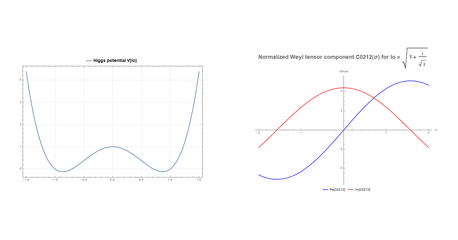
where V is the classical Higgs potential and the broken symmetry in the system can be interpreted as an apparent mismatch of coefficients related to . The Figure 1 shows the classic "Mexican sombrero" potential . Since is related in equation (43) to the angle describing the spin, this means that in this solution the spin effect of the field is described by invariant angle (depends only on ) and, according to (55) it is closely related to the trace of the metric and, consequently, to the Ricci scalar in the curvilinear description and thus to spacetime curvature. This also at least means that to obtain correct results in curved spacetime in the Alena Tensor model, the Higgs-like field is needed. Perhaps the above result will help explain the existence of the Higgs field and its relationship to curvature and spin.
For the whole metric becomes significantly simplified and symmetric
which means that it may be assumed that the Higgs boson is probably related to the curvature of spacetime, corresponding to this configuration.
Using hyperbolic identities and expressing
then using (33) one obtains
Using (37) and (38), the releation between electromagnetic energy density , angle and spin four-vector zero component is therefore
which explains the origin of and the connection of spin and Lagrangian with the energy density of the electromagnetic field. Since, according to the considered approach of Alena Tensor, in curved spacetime the energy density expressed by must vanish (the entire stress-energy tensor of the electromagnetic field vanishes), this means, that and thus becomes invariant, which allows to analyze the transition to curved spacetime.
One may now consider what value the Alena Tensor takes in curved spacetime. To do this, it is easiest to analyze the behavior of . As one may calculate, the determinant of this tensor is 0 and the matrix rank is 2, but, as described in the introduction, it degenerates to in curved spacetime. It can be seen that in the Alena Tensor approach the metric follows from propagation. However, in curved spacetime the electromagnetic field according to this approach should vanish, remaining present only in the metric and determining geodetic. This can be achieved by degenerating vectors and to a single vector in curved spacetime . However, in such situation the equation (45) forces this vector to be the four-velocity, divided by the Lorenz factor
which degenerates from (46) to the form
Since the metric is known and may be expressed by values of , in flat spacetime thanks to (45) this allows to easy obtain the Einstein tensor and Ricci tensor using the equation (10).
The described system seems to be Petrov type D or II [29], although to be sure, the Weyl tensor should be calculated. This does not seem possible for the general case (without auxiliary assumptions about symmetries), but one could simplify the obtained description considerably, based on the following observation. One may notice, that the vanishing Lorentz factor in can be interpreted as an important suggestion for the description of motion in curved spacetime. Such motion would correspond to a stream of particles moving without dilation, a strictly ordered flow without local perturbations, resembling a perfect, infinitely stiff fluid. This means that should be the Killing tensor and the system schould have hidden symmetry (similar to the Carter constant in Kerr solutions).
As shown previously, product of the basis is in considered case , which means that null vectors have global significance for spacetime geometry, thus Killing tensor should have a strong connection with propagation along null vectors (it is not a random symmetry, but a deep feature of spacetime) and this would mean the existence of special wave surfaces, e.g. electromagnetic waves and/or gravitational radiation. This would be a also clear indication that spacetime belongs to the Petrov D or II class and is associated with wave propagation solutions.
Also, the analysis of obtained equations drive to conclusion, that energy (energy density) is not something external to geometry in Alena Tensor approach, but energy is defined by the geometry of spacetime itself. This is a result in the spirit of General Relativity, but it goes even deeper: metric depends on , but at the same time depends on the metric because it is trace of in this metric. The system itself defines its own energy through the structure of the field, which is similar to the idea of self-consistent field [30] - where the field and the source are inseparable, or emergent gravity [31] - where energy, gravity and geometry arise from a common structure, or induced geometry [32] - where energy comes from deformation of spacetime itself, as e.g. in Sakharov’s theory [33]. It is impossible to “decree” energy in Alena Tensor, it must be calculated from geometry and the system works as a closed causal cycle.
The dependence for of its norm and trace in curved spacetime (the norm is the square of the trace) is a key property for null space and suggests that describes isometries related to null wave propagation, similar to pp-wave [34] and Robinson-Trautman solutions [35], what is actually expected in considered approach based on electromagnetic stress-energy tensor and result (51). This would also mean that the Killing tensor is directly related to the energy distribution in spacetime as expected, similar to other GR solutions (eg. Kerr solution), and lead to a rather groundbreaking but also expected result in the context of the discussed approach, that the Killing tensor directly determines the Einstein tensor in main GR equation.
Since is simply the Alena Tensor (stress-energy tensor for the system) divided by , it gives correct conserved values in the Noether formalism (conserved density of energy and momentum). From the definition of the Alena Tensor as the energy-momentum tensor for a system it also follows that is symmetric and vanishes.
Since this implies that along a geodesic parametrized by proper time , its total derivative vanishes.
Using the symmetry of one may note that
Therefore, the condition
holds for arbitrary tangent vectors , and it follows that . Therefore normalized Alena Tensor is Killing tensor for considered system.
In this way Alena Tensor theory becomes equivalent to some specific case of General Relativity equation expressed in the following form
where according to (10) in the above equation is the classical Einstein tensor . Thanks to the above, since the Weyl tensor is defined as the part of the Riemann tensor that does not depend on the Ricci tensor, this implies that since Killing tensor determines the Einstein tensor, and the Einstein tensor determines the Ricci tensor, then one could calculate the Weyl tensor by extracting the part of the curvature that does not contain the Ricci tensor. One may expect that the Weyl tensor calculated in this way should depend on the energy density, the cosmological constant and the null vectors, which would mean that the spacetime geometry is strongly related to the energy of the electromagnetic field, exactly as seen in the obtained equations. This would also mean that the Christoffel symbols can be expressed as a function of the Killing and Einstein tensors, and the Riemann tensor can be written directly as a function of the Ricci and Killing tensors.
For the system under consideration, one may therefore construct a general Weyl tensor ansatz, which must contain only components that do not become zero when the trace part is subtracted from the Riemann tensor. It should be of the form
where
It is easy to check that the above tensors are linearly independent and form the basis for the representation of any Weyl tensor in the system under consideration. Analysis of their behavior indicates that
- is responsible for "pure" directional propagation - e.g. a gravitational wave propagating along null directions (purely conformal part of the Weyl tensor — described solely by null geometry),
- describes non-radiating, "axial" deformation of space - e.g. tidal sequences, consistent with mass motion without undulations,
- describes conformal distortion of the background metric itself.
The coefficients , , are not known a priori, but one may determine them with help of Riemann tensor. To calculate the Riemann tensor in the system under consideration, it is enough to assume the following ansatz
It has the following justification
- The Riemann tensor satisfies the known algebraic symmetries: The above ansatz satisfies them automatically.
- There are only two tensor objects available in the system: the metric and the Killing tensor . The Riemann tensor must be constructed exclusively from them.
- The first term with corresponds to the geometry of a space with constant curvature, as in de Sitter space:
- The second term with is the minimal geometrically correct extension that takes into account the presence of non-null energy (represented by ). Its construction provides correct symmetries and enables the reproduction of a non-null Ricci tensor
- Other possible combinations (e.g. ) are linearly dependent or asymmetric with respect to the required properties of the Riemann tensor — they do not provide new information in the case under consideration.
- The whole creates the most general fourth-order tensor with Riemann symmetries, which can be constructed from available geometric objects.
Comparing the Ricci scalar and obtained from anstaz and the one obtained from GR equation with Alena Tensor, one obtains coefficients . Their complex structure does not allow for inclusion in this article, but they can be read in the supplementary files, which allows for further analysis. Given the Riemann tensor and computing the trace part of the Riemann tensor, one obtains the Weyl tensor in generalized form for the system under consideration. Normalized Riemann and Weyl tensors (divided by the cosmological constant) were computed in the supplementary files.
Having calculated the above-mentioned tensors, one may substitute an example basis (50) depending on and solve the system of equations (33, 41, 56) presenting the results only as a function of and . Due to the complex relationships between variables, analytical solution is presented in supplementary file, and Weyl tensor component values were calculated for an example value of from (57). The Figure 2 below clearly shows the wave nature of the component of the Weyl tensor, presenting the result of the calculations performed and it actually seems, that the Weyl tensor component encodes the variation of some curvature field along the propagating direction . Table 1 presents the values of the key components of the Weyl tensor calculated for the value adopted for the analysis.
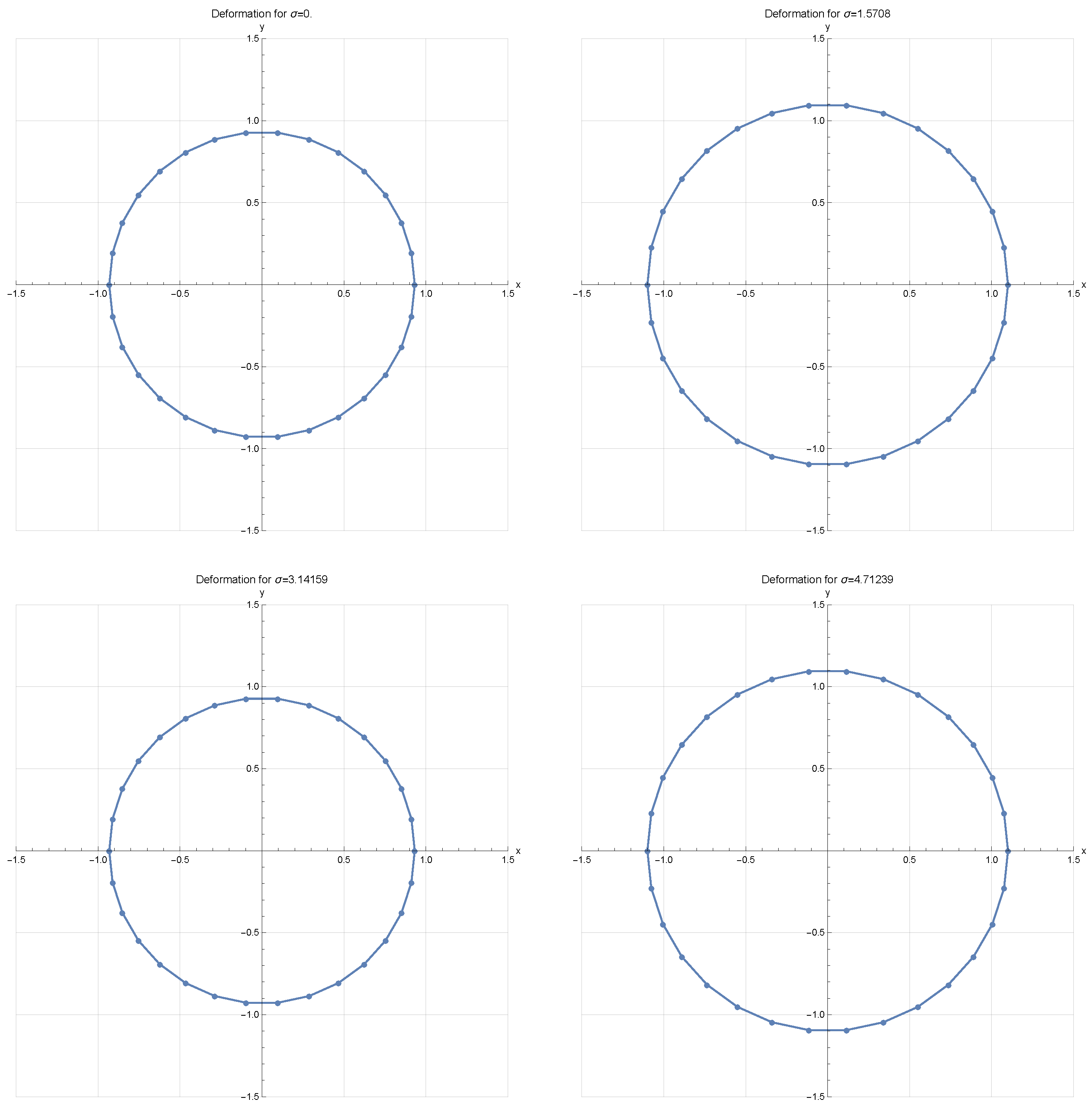
By calculating the Penrose–Newman scalars one can conclude that the example system described by the above Weyl tensor is Petrov type II and does indeed contain gravitational waves with two polarizations (+ and x), as well as some observable symmetries. The next two graphs show the oscillations of these scalars and the deformation effects for an example arrangement of test particles on a circle. In the supplementary materials there is a gif file presenting an animation of this distortion. This animation reveals the typical quadrupolar nature of spacetime distortions induced by gravitational waves (characteristic twisting and stretching).
The above Weyl tensor components are actually normalized. One may thus present the main GR equation in the Alena Tensor notation (10) and represent it using the vacuum pressure as follows
Since the obtained Weyl tensor is normalized by , this means that the interpretation from (18) that gravitational waves in the Alena Tensor are in fact propagating vacuum pressure disturbances also seems to be correct.
It is also worth noting that the obtained metric term can in principle be interpreted as a vacuum energy contribution (effective cosmological constant) as in [36,37] playing the role of a metric scaling factor, as e.g. described in [38] which allows to conclude about the value of the second invariant of the electromagnetic field.
Additionally, one may invoke the scalar field associated with the presence of matter, where . It is known from 2.2 that is responsible for the presence of sources and in their absence . Therefore, interpreting whole as the wave amplitude tensor one would get representation which would also allow to search for as a certain wave function.
Figure 4.
Deformation visualization for particles on a circle.
This approach allows for two simplifications related to the analysis of gravitational waves. Considering the force responsible for effects related to gravity as shown in (12) and extracting the acceleration from it, one gets
since according amendment from [10] .
As shown in [9], is directly related to the effective potential in gravitational systems which can be calculated from the GR equations. This would allow searching for propagating changes of the effective potential itself () similarly as was postulated in [39]. It would significantly simplify both the calculations and perhaps the methods of detecting gravitational waves.
The second potential simplification results from the possibility of analyzing only the Poynting four-vector as which might also help simplify the calculations and look for experimental proof of correctness for the Alena Tensor approach.
4. Conclusion and Discussion
As shown in the above article, the Alena Tensor ensures the existence of gravitational waves and allows their physical interpretation, providing key tools for their further analysis including the ability to calculate and visualize Weyl tensor components. The obtained decomposition of the electromagnetic field stress-energy tensor (51) allows for further analysis of metrics for curved spacetime and also to use the proposed null basis for further development in the framework of conformal geometry, the NP formalism and the description of photons in QFT. It also seems reasonable to generalize above results for non-linear electromagnetism using e.g. approach presented in [40] and search for a description of elementary particles that will provide relatively stable solutions to the obtained equations, perhaps also taking into account new approaches, such as those proposed in [41].
It remains an open question whether the Alena Tensor is a correct way to describe physical systems, but this paper shows that it exhibits many properties that are expected from such a description, including the existence of gravitational waves whose behavior corresponds to GR. Additionally, quite surprisingly, it naturally forces the existence of the Higgs field and this field turns out to be necessary to even consider curved spacetime and gravitational waves. The connection between Alena Tensor and the Killing tensor obtained in this paper reveals a deep, nonlinear connection between the matter distribution and the geometry and symmetries of spacetime. These results show that the matter distribution is not arbitrary, but precisely tuned to the geometry and hidden symmetries of spacetime, which allows for their further analysis in the language of Killing tensors and conformal Weyl curvature.
5. Statements
All data that support the findings of this study are included within the article (and any supplementary files).
During the preparation of this work the author did not use generative AI or AI-assisted technologies.
Author did not receive support from any organization for the submitted work.
Author have no relevant financial or non-financial interests to disclose.
List of Figures
| 1. The existence of the Higgs field potential as a consequence of | 11 |
| 2. Weyl tensor C0212 component as a wave. | 14 |
| 3. Oscillations of Penrose–Newman scalars. | 15 |
| 4. Deformation visualization for particles on a circle. | 16 |
Supplementary Materials
The following supporting information can be downloaded at the website of this paper posted on Preprints.org.
References
- Bailes, M.; Berger, B.K.; Brady, P.; Branchesi, M.; Danzmann, K.; Evans, M.; Holley-Bockelmann, K.; Iyer, B.; Kajita, T.; Katsanevas, S.; et al. Gravitational-wave physics and astronomy in the 2020s and 2030s. Nature Reviews Physics 2021, 3, 344–366. [Google Scholar] [CrossRef]
- Schutz, B.F. Gravitational wave astronomy. Classical and Quantum Gravity 1999, 16, A131. [Google Scholar] [CrossRef]
- Grant, A.M.; Nichols, D.A. Outlook for detecting the gravitational-wave displacement and spin memory effects with current and future gravitational-wave detectors. Physical Review D 2023, 107, 064056. [Google Scholar] [CrossRef]
- Borhanian, S.; Sathyaprakash, B. Listening to the universe with next generation ground-based gravitational-wave detectors. Physical Review D 2024, 110, 083040. [Google Scholar] [CrossRef]
- Milgrom, M. Gravitational waves in bimetric MOND. Physical Review D 2014, 89, 024027. [Google Scholar] [CrossRef]
- Tahura, S.; Nichols, D.A.; Yagi, K. Gravitational-wave memory effects in Brans-Dicke theory: Waveforms and effects in the post-Newtonian approximation. Physical Review D 2021, 104, 104010. [Google Scholar] [CrossRef]
- Matos, I.S.; Calvão, M.O.; Waga, I. Gravitational wave propagation in f (R) models: New parametrizations and observational constraints. Physical Review D 2021, 103, 104059. [Google Scholar] [CrossRef]
- Shapiro, I.L.; Pelinson, A.M.; de, O. Salles, F. Gravitational waves and perspectives for quantum gravity. Modern Physics Letters A 2014, 29, 1430034. [Google Scholar] [CrossRef]
- Ogonowski, P.; Skindzier, P. Alena Tensor in unification applications. Physica Scripta 2024, 100, 015018. [Google Scholar] [CrossRef]
- Ogonowski, P. Proposed method of combining continuum mechanics with Einstein Field Equations. International Journal of Modern Physics D 2023, 2350010, 15. [Google Scholar] [CrossRef]
- Ogonowski, P. Developed method: interactions and their quantum picture. Frontiers in Physics 2023, 11, 1264925. [Google Scholar] [CrossRef]
- Logunov, A.; Mestvirishvili, M. Hilbert’s causality principle and equations of general relativity exclude the possibility of black hole formation. Theoretical and Mathematical Physics 2012, 170, 413. [Google Scholar] [CrossRef]
- Friedman, Y. Superposition principle in relativistic gravity. Physica Scripta 2024, 99, 105045. [Google Scholar] [CrossRef]
- Poplawski, N.J. Geometrical formulation of classical electromagnetism. arXiv preprint arXiv:0802.4453 2008.
- Chang, Y.F. Unification of gravitational and electromagnetic fields in Riemannian geometry. arXiv preprint arXiv:0901.0201 2009.
- Chernitskii, A.A. On unification of gravitation and electromagnetism in the framework of a general-relativistic approach. arXiv preprint arXiv:0907.2114 2009.
- Kholmetskii, A.; Missevitch, O.; Yarman, T. Generalized electromagnetic energy-momentum tensor and scalar curvature of space at the location of charged particle. arXiv preprint arXiv:1111.2500 2011.
- Novello, M.; Falciano, F.; Goulart, E. Electromagnetic Geometry. arXiv preprint arXiv:1111.2631 2011.
- de Araujo Duarte, C. The classical geometrization of the electromagnetism. International Journal of Geometric Methods in Modern Physics 2015, 12, 1560022. [Google Scholar] [CrossRef]
- Hojman, S.A. Geometrical unification of gravitation and electromagnetism. The European Physical Journal Plus 2019, 134, 526. [Google Scholar] [CrossRef]
- Woodside, R. Space-time curvature of classical electromagnetism. arXiv preprint gr-qc/0410043 2004.
- Bray, H.; Hamm, B.; Hirsch, S.; Wheeler, J.; Zhang, Y. Flatly foliated relativity. arXiv preprint arXiv:1911.00967 2019.
- Jafari, N. Evolution of the concept of the curvature in the momentum space. arXiv preprint arXiv:2404.08553 2024.
- Kaur, L.; Wazwaz, A.M. Similarity solutions of field equations with an electromagnetic stress tensor as source. Rom. Rep. Phys 2018, 70, 1–12. [Google Scholar]
- MacKay, R.; Rourke, C. Natural observer fields and redshift. J Cosmology 2011, 15, 6079–6099. [Google Scholar]
- Ahmadi, N.; Nouri-Zonoz, M. Massive spinor fields in flat spacetimes with nontrivial topology. Physical Review D—Particles, Fields, Gravitation, and Cosmology 2005, 71, 104012. [Google Scholar] [CrossRef]
- Waluk, P.; Jezierski, J. Gauge-invariant description of weak gravitational field on a spherically symmetric background with cosmological constant. Classical and Quantum Gravity 2019, 36, 215006. [Google Scholar] [CrossRef]
- Anghinoni, B.; Flizikowski, G.; Malacarne, L.C.; Partanen, M.; Bialkowski, S.; Astrath, N.G.C. On the formulations of the electromagnetic stress–energy tensor. Annals of Physics 2022, 443, 169004. [Google Scholar] [CrossRef]
- Hall, G. Wave Surface Symmetry and Petrov Types in General Relativity. Symmetry 2024, 16, 230. [Google Scholar] [CrossRef]
- Ignat’ev, Y.G. The self-consistent field method and the macroscopic universe consisting of a fluid and black holes. Gravitation and Cosmology 2019, 25, 354–361. [Google Scholar] [CrossRef]
- Padmanabhan, T. Emergent gravity paradigm: recent progress. Modern Physics Letters A 2015, 30, 1540007. [Google Scholar] [CrossRef]
- Eichhorn, A.; Surya, S.; Versteegen, F. Induced spatial geometry from causal structure. Classical and Quantum Gravity 2019, 36, 105005. [Google Scholar] [CrossRef]
- Sakharov, A.D. Vacuum quantum fluctuations in curved space and the theory of gravitation. General Relativity and Gravitation 2000, 32, 365–367. [Google Scholar] [CrossRef]
- Sämann, C.; Steinbauer, R.; Švarc, R. Completeness of general pp-wave spacetimes and their impulsive limit. Classical and Quantum Gravity 2016, 33, 215006. [Google Scholar] [CrossRef]
- Davidson, W. Robinson–Trautman solutions to Einstein’s equations. General Relativity and Gravitation 2017, 49, 1–4. [Google Scholar] [CrossRef]
- Wang, Q. Reformulation of the cosmological constant problem. Physical Review Letters 2020, 125, 051301. [Google Scholar] [CrossRef]
- Gueorguiev, V.G.; Maeder, A. Revisiting the Cosmological Constant Problem within Quantum Cosmology. Universe 2020, 6, 108. [Google Scholar] [CrossRef]
- Marsh, A. Defining geometric gauge theory to accommodate particles, continua, and fields. Journal of Mathematical Physics 2024, 65. [Google Scholar] [CrossRef]
- Domènech, G. Scalar induced gravitational waves review. Universe 2021, 7, 398. [Google Scholar] [CrossRef]
- Lindgren, J.; Kovacs, A.; Liukkonen, J. Electromagnetism as a purely geometric theory. In Proceedings of the Journal of Physics: Conference Series. IOP Publishing, 2025, Vol. 2987, p. 012001.
- Rakitzis, T.P. Spatial wavefunctions of spin. Physica Scripta 2023. [Google Scholar] [CrossRef]
Figure 1.
The existence of the Higgs field potential as a consequence of .
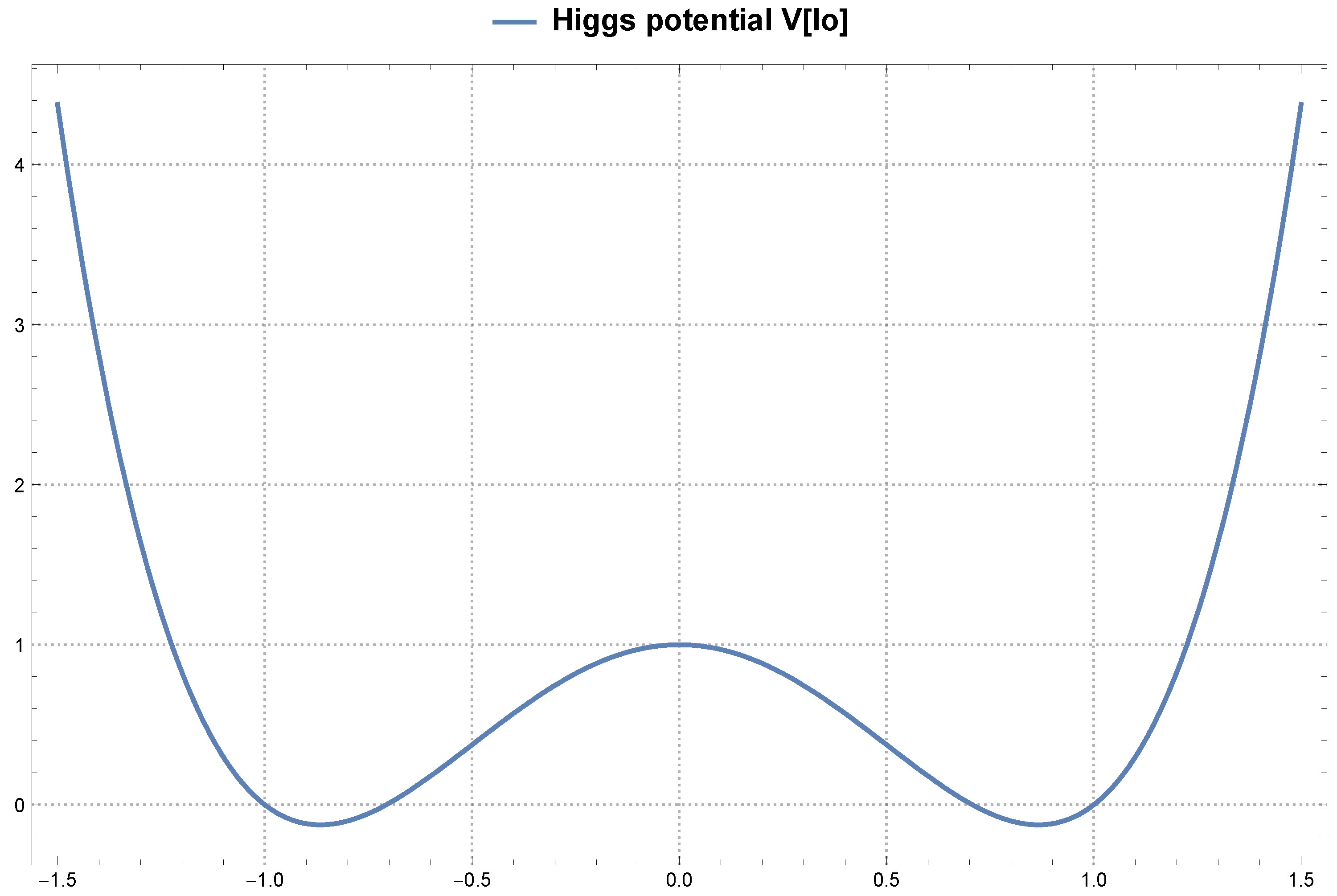
Figure 2.
Weyl tensor component as a wave.
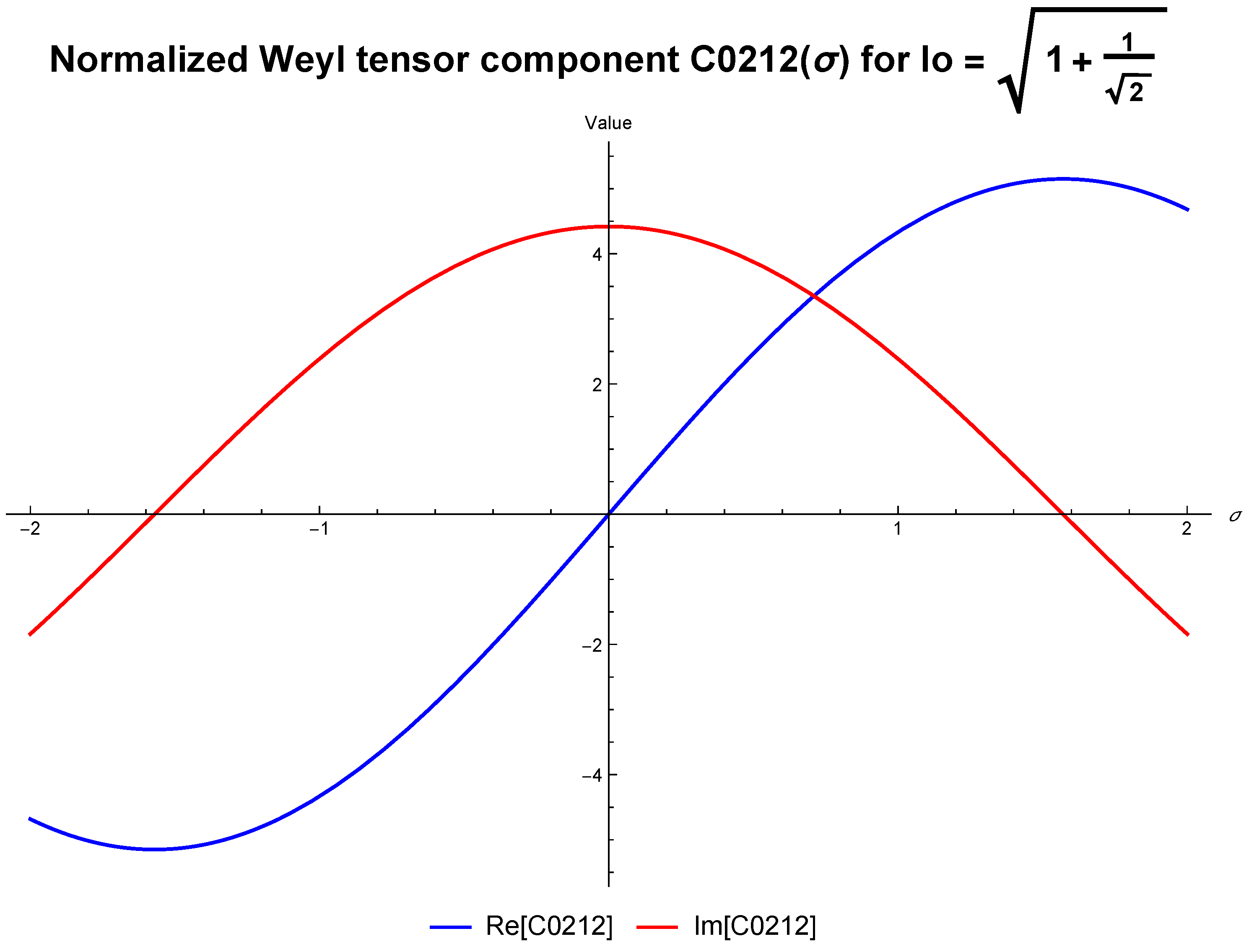
Figure 3.
Oscillations of Penrose–Newman scalars.
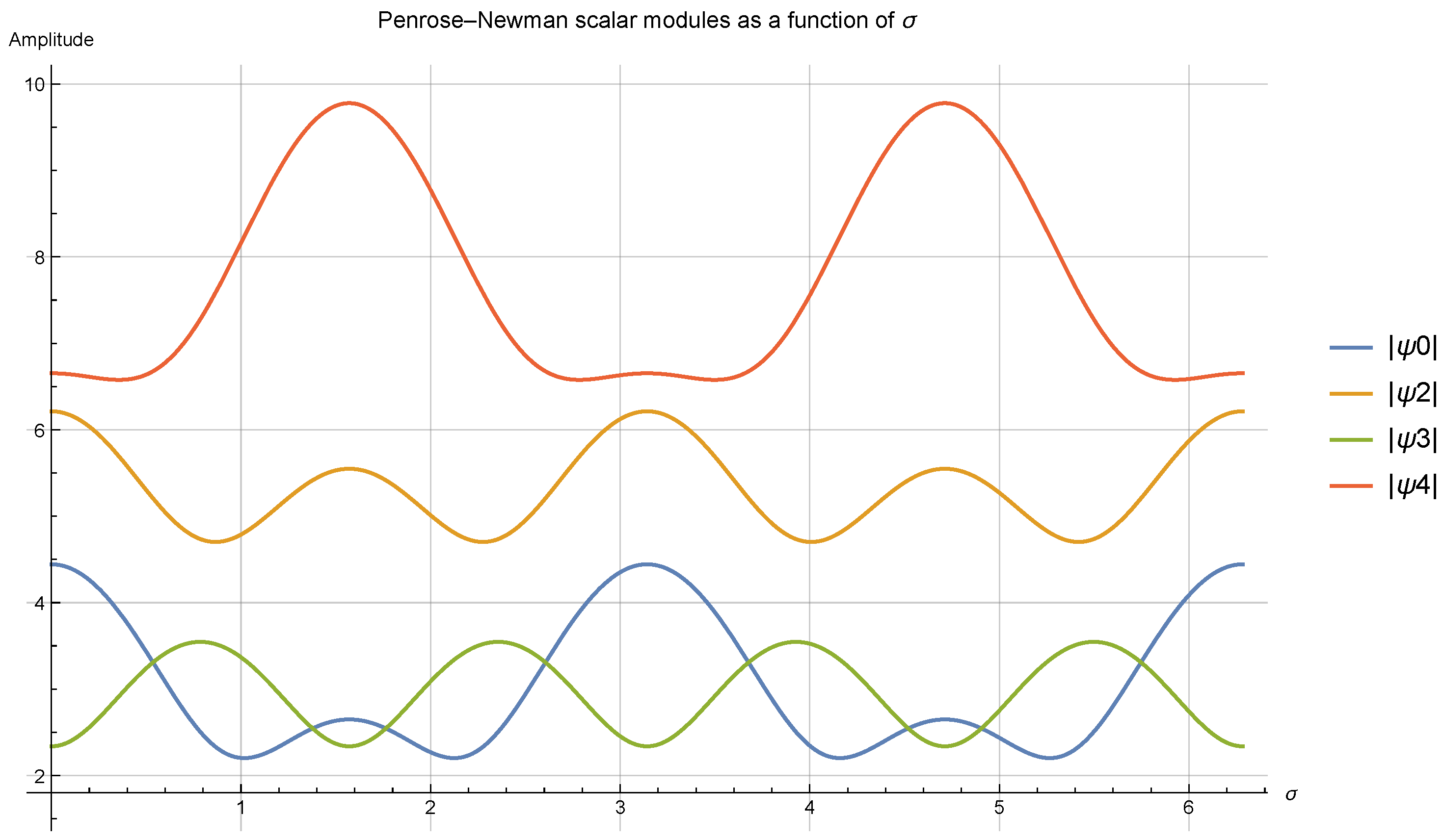

Table 1.
Component values of the Weyl tensor as functions of the angle for selected value.
| Component | Value |
|---|---|
| 0 | |
Disclaimer/Publisher’s Note: The statements, opinions and data contained in all publications are solely those of the individual author(s) and contributor(s) and not of MDPI and/or the editor(s). MDPI and/or the editor(s) disclaim responsibility for any injury to people or property resulting from any ideas, methods, instructions or products referred to in the content. |
© 2025 by the authors. Licensee MDPI, Basel, Switzerland. This article is an open access article distributed under the terms and conditions of the Creative Commons Attribution (CC BY) license (http://creativecommons.org/licenses/by/4.0/).
Copyright: This open access article is published under a Creative Commons CC BY 4.0 license, which permit the free download, distribution, and reuse, provided that the author and preprint are cited in any reuse.


