
Submitted:
16 August 2025
Posted:
20 August 2025
You are already at the latest version
Abstract
Alena Tensor is a recently discovered class of energy-momentum tensors that proposes a general equivalence of the curved path and geodesic for analyzed spacetimes which allows the analysis of physical systems in curvilinear, classical and quantum descriptions. In this paper it is shown that Alena Tensor is related to the Killing tensor K and describes the class of GR solutions G + Λ g = 2 Λ K. In this picture, it is not matter that imposes curvature, but rather the geometric symmetries, encoded in the Killing tensor, determine the way spacetime curves and how matter can be distributed in it. It was also shown, that Alena Tensor gives decomposition of energy-momentum tensor of the electromagnetic field using two null-vectors and in natural way forces the Higgs-like potential to appear. The obtained generalized metrics (covariant and contravariant) allow for further analysis of metrics for curved spacetimes with effective cosmological constant. The obtained solution can be also analyzed using conformal geometry tools. The calculated Riemann and Weyl tensors allow the analysis of purely geometric aspects of curvature, Petrov-type classification, and tracking of gravitational waves independently of the matter sources. It has also been shown that the total power emitted from the gravitational system in the form of gravitational waves fully corresponds to the results obtained in GR allowing for a significant simplification of calculations for gravitational waves. The existing results for electromagnetism and gravity were also arranged and reformulated based on principle of least action, and the directions of generalization to all gauge fields were discussed. The article has been supplemented with a file containing a computational notebook used for symbolic derivations which may help in further analysis of this approach.
Keywords:
Alena Tensor
; Gravitational waves
; General Relativity
; Electromagnetism
; Higgs field
1. Introduction
Gravitational waves are a well-understood and researched issue [1], and it seems that the area of this research will develop dynamically both in theoretical understanding [2,3] and methods of waves detection [4,5]. While there is much evidence that General Relativity is (so far) the best description of relativistic gravity, the analysis of gravitational waves provides further evidence and is an important area of research, providing significant information about physical systems. The ability to describe gravitational waves is also an important requirement for alternative to GR theories [6,7,8] and the theories of quantum gravity [9].
Alena Tensor is in the early stages of research. It is a recently discovered class of energy-momentum tensors that allows for equivalent description and analysis of physical systems in flat spacetime (with fields and forces) and in curved spacetime (using Einstein Field Equations) proposing the overall equivalence of the curved path and the geodesic. In this method it is assumed that the metric tensor is not a feature of spacetime, but only a method of its mathematical description. In previous publications [10,11,12] it was already shown that this approach allows for a unified description of a physical system (curvilinear, classical and quantum) ensuring compliance with GR and QM equations. Due to this property, the Alena Tensor seems to be a useful tool for studying unification problems, quantum gravity and many other applications in physics.
Many researchers try to reproduce GR equations in flat spacetime or vice versa [13,14] also many researchers try to incorporate electromagnetism into GR, connecting it in many ways with the geometry of spacetime [15,16,17,18,19,20,21,22]. There are known such approaches on the basis of differential geometry [23,24,24], based on field equations [25,26] as well as promising analyses of spinor fields [27] or helpful approximations for a weak field [28]. For this reason, the Alena Tensor should be viewed as a useful tool that can help in the development of many different approaches or, potentially, as an independent theory requiring theoretical and experimental verification. Therefore it seems worth checking whether the this approach ensures the existence of gravitational waves and what their interpretation is.
Another important reason for writing this article is the fact that although the Alena Tensor equations provide consistency with the Einstein Field Equations in curved spacetime, the description of curvilinear solutions provided by this approach has not been sufficiently discussed in the literature so far. The description of gravitational waves, due to the required mathematical apparatus, will allow to deepen knowledge of this approach and to narrow down the classes of GR solutions that are consistent with it. Such a description will not provide full knowledge about unification, because full unification is not a task for one article and will probably require many years of cooperation of the scientific community. However, this article has the potential to take another step towards unification using the Alena Tensor, providing theoretical tools and hints for further research on unification using this approach.
In this paper it will be analyzed the possibility of describing gravitational waves using the Alena Tensor. Due to the fact that research on this approach is a relatively young field, to facilitate the analysis of the article, the next section summarizes the results obtained so far and introduces the necessary notation. All computationally difficult equations and graphs can be found in the attached supplementary material as computational notebook.
In the Results section, at first it will be shown that the use of the Alena Tensor leads to the decomposition of the electromagnetic field stress-energy tensor into components dependent on two null vectors. Next, the general form of the metrics for curved spacetime described by the Alena Tensor will be obtained, the Riemann and Weyl tensors will be calculated and presented for an example field configuration. It will also be shown that obtained gravitational waves correspond to the GR predictions and the correct operation of the Alena Tensor requires the existence of the Higgs-like potential. In the last part it will be calculated that the total power radiated from the gravitational system described by Alena Tensor fully corresponds to the results obtained in GR. The article also presents tables and graphs illustrating the obtained results (Higgs potential, Weyl tensor components, Newman-Penrose scalars) and it was shown, that the analysis of the equations lead to the conclusions contained in the abstract.
Although at the first moment the paradigm shift proposed by this approach may seem incomprehensible, the author hopes that the reader will trust the scientific method, which encourages us to calculate and check everything based on the correctness of the results obtained.
2. Organizing and Interpreting the Alena Tensor Previous Results for Electromagnetism
To provide an introduction to Alena Tensor approach, one may first systematize and organize the conclusions drawn from previous research on as systems with only electromagnetic field. In the last section, the possibility of generalizing this approach to all gauge fields will be discussed. The author uses the metric signature (+,-,-,-).
2.1. Transforming a Curved Path into a Geodesic
It is worth starting the analysis with a postulate concerning the field invariant, which follows directly from Equation (28) in [11]. Considering a system with only an electromagnetic field as an example, denoting the electromagnetic field as and denoting the metric tensor by means of which the physical system is analyzed as , one may denote the invariant of this field as . Let this field invariant be defined dually as follows
where is some unknown constant and where , as raised in [11], in this approach is a metric tensor describing a curved spacetime in which all motion occurs along geodesics. By making variation on with respect to metric (Hilbert’s method) one obtains the energy-momentum tensor of the electromagnetic field denoted as , which can be expressed dually as
As can be seen, such approach establishes a relationship between the field and the metric tensor and in the spacetime described by the metric tensor , one obtains . The value of becomes thus constant only for such field configuration, therefore in the limit for electromagnetic field tensor vanishes, maintaining continuity of function. This is quite important, because most calculations in curved spacetime are performed under the assumption that the variation of the constant does not vanish. This is indeed true, with one above exception, where the constancy follows precisely from the limit.
In this way one obtains a generalized description of the field stress-energy tensor which has the following properties
- in flat spacetime is the usual, classical energy-momentum tensor of the electromagnetic field
- its trace vanishes in any spacetime, regardless of the considered metric tensor
- in spacetime for which the entire tensor vanishes
- which is expected property of the metric tensor (it was already shown in [11] that indeed may be considered as metric tensor for curved spacetime).
Such approach also means that every field stress-energy tensor could naturally satisfy the Israel junction condition for hypersurface [29]. For example, in electromagnetism this provides the possibility of viewing as a certain hyperspace, where actually describes a discontinuity, eg. , so the system could satisfy the holographic principle [30] and the entire volume dynamics could be described by the surface theory and vice-versa. It will be shown later that such a perception of may be a simple explanation for Alena Tensor.
The second important postulate underlying the Alena Tensor is an amendment to continuum mechanics introduced in Equation (11) of [11]. Assuming as rest mass density, four-momentum density is defined as what takes into account motion and Lorentz contraction of the volume. Total four-force density acting on matter is therefore defined as
As shown in [11], the above amendment thus introduces a natural property concerning curved spacetime
The above property means that the field is indeed not needed in curved spacetime and can only manifest itself through curvature. This also means that the four-currents have the form where denotes the rest density of the transferred charge, which ensures the continuity equation.
The final postulate that explains the results obtained so far is the assumption that the density of matter is not a value independent of the field, but is in fact a manifestation of the existence of the field, and without fields, matter does not exist. This assumption is consistent with the general idea of Quantum Mechanics, in which particles are de facto quanta of the field and it was also raised in [11]. In the system with only electromagnetic field one may thus define matter density linking it to electric susceptibility as
where one may recall from [10] other coefficients related to the electromagnetic field
- relative permittivity
- relative permeability
- volume magnetic susceptibility
This approach allows to associate the momentum density with a certain four-current what makes it dependent on the metric .
Defining the Lagrangian density for the system as
and making variations with respect to the metric (Hilbert’s method), using the three postulates mentioned earlier, one obtains Alena Tensor for the system
where is energy-momentum tensor of the system, which can be analyzed independently of the used for analysis. Its vanishing four-divergence can be considered both in flat spacetime and in curved spacetime. One may therefore denote the four-force densities due to the field in flat spacetime, where
- is the density of the electromagnetic four-force
- was shown in [10] as related to the presence of gravity in the system.
and where vanishing four-divergence of in flat spacetime results from the balance of the four-force densities
In curved spacetime () one obtains thus the forces due to the field are replaced by Christoffel symbols of the second kind corresponding to curvature related to the metric tensor defined by the filed according to (2) and (4).
The reasoning carried out above for electromagnetism is universal and creates possibility to consider dually also energy-momentum tensors associated with all gauge fields, what will be shown further.
2.2. Connection with Continuum Mechanics, GR and QFT/QM
In the sense of Continuum Mechanics, may be considered as a density of the volume four-forces, while the may be considered as a density of surface four-forces, related to hyperspace described by , where surface waves are driven by the gradient of the pressure. To make the Alena Tensor consistent with Continuum Mechanics in flat spacetime, it is thus enough to define negative pressure p as in [11], . Such substitution yields
where is the metric tensor of flat Minkowski spacetime. Introducing deviatoric stress tensor one obtains relativistic equivalence of Cauchy momentum equation (convective form) in which only appears as a pure volume force (body force)
One may therefore construct a Lagrangian whose variation provides the tensor responsible for the four-force density understood as
It may be obtained with the use of the interpolating path method based on path parameter , where the path is . Using this method one obtains
where
Since whole contribution for integral is only for , thus
As one may notice, integrates along the deformation path and reflects the total deformation effect, which can be identified with the effective ”surface forces” at the boundary of the metric space. Therefore tensor, created with by variation over the metric gives a four-dimensional equivalent to the Cauchy tensor, which gives a local description of the energy-momentum and stress flows. Its spatial part on the surface t=const can be thus identified as the equivalent of the Cauchy tensor of mechanical stresses. In this perspective, Lagrangian is responsible for all forces due to the field , and Lagrangian is responsible for . This reflects the classical division into the Lagrangian of matter and fields, although in this approach the existence of matter is also a consequence of the existence of the fields, and because the four-divergences of the tensors resulting from them cancel each other out.
The above also provides a connection to General Relativity in curved spacetime. For this purpose, one may introduce the following tensors, which can be analyzed in both flat and curved spacetime
Above allows to rewrite Alena Tensor making variations with respect to the metric on following Lagrangian density to obtain
As can be seen, the tensor may be constructed with the use of Hilbert’s method (for any ), however alone and cannot be constructed this way, because it is impossible to construct such a tensor in a general way by forcing an additional trace of in the prior Lagrangians. The only spacetime in which Hilbert’s method allows the derivation of alone is curved spacetime (), where is constant, it is therefore possible to correct the obtained tensors with a Lagrangian constructed from a constant.
Analyzing the above equation in curved spacetime (), one obtains simplifications
thus above can be interpreted in curved spacetime as the main equation of General Relativity up to the constant where and can be interpreted in curved spacetime, respectively, as Einstein curvature tensor and Ricci tensor both with an accuracy of constant. However, in this approach R is not a source Lagrangian density for tensor .
Denoting in general case
one may rewrite (18) as
where the trace of must give R, since the whole term in the brackets describes the field
thus must have vanishing trace and the whole term vanishes in curved spacetime. For this reason in curved spacetime and must be related to and R plays the role of invariant of this field tensor.
Indeed, analyzing the tensor in flat spacetime () one can notice, that it is related to the non-body forces seen in the description of the Cauchy momentum equation
which means that in the Alena Tensor analysis method gravity is not a body force, and as shown in [10] in above
- is the density of the radiation reaction four-force
- is density of the four-force related to gravity, where
- is related to the effective potential in the system with gravity.
It can be calculated that vanishes in two cases:
- - which turns out to be the case of free fall
- which occurs in the case of circular orbits
Neglecting the electromagnetic force and the radiation reaction force, using the above equation one can reproduce the motion of bodies in the effective potential obtained from the solutions of General Relativity. Such a description has already been done for the Schwarzschild metric [10] for
where is a certain constant. The solutions obtained in this way enforce the existence of gravitational waves due to time-varying (except for free fall and circular orbits). As will be shown later in the article, such a description of gravity can be generalized and allows for a correct description of both the motion and the energy radiated by gravitational waves.
In the above description, gravity itself is not a force, because the above description is based on an effective potential. However, one can see a similarity to Newton’s classical equations for the stationary case with a stationary observer, for which can be approximated by Newton’s gravitational force with the opposite sign. Thus for stationary observer represents a force that must exist to keep a stationary observer suspended above the source of gravity in fixed place.
The description of gravity obtained from Alena Tensor is surprisingly consistent with current knowledge both in flat and curved spacetime, despite the fact that gravity itself in this description in flat spacetime is not a force, and the force is not a body force but is related to surface forces on some hyperspace.
The Alena Tensor constructed in presented way according to [10,12] may be also represented in flat spacetime as a symmetric Noether tensor using the obtained properties of the electromagnetic field. Denoting as the Lagrangian for computing the Noether tensor, Alena Tensor may be simplified in flat spacetime to
where is known four-potential ensuring required symmetry of such Noether tensor, which allows analysis in classical field theory and quantum theories. Obtained canonical four-momentum provides and to consider charged particles one may use
where is four-momentum, is pressure-volume work, and where and are in fact two gauges of electromagnetic four-potential. Mentioned previously four-potential where is responsible for the force associated with gravity and radiation reaction force. It was also shown that canonical four-momentum may be expressed as
where due to its property , seems to be some description of rotation or spin, and where describes the transport of energy due to the field.
The quantum picture obtained from the Alena Tensor [10,12] for the system with electromagnetic field leads to the conclusion that gravity and the radiation reaction force have always been present in Quantum Mechanics and Quantum Field Theory. This conclusion follows from the fact that the quantum equations obtained from the Alena Tensor for the system with electromagnetic field [10] are actually the three main quantum equations currently used:
-
simplified Dirac equation for QED:
- Klein-Gordon equation,
- equivalent of the Schrödinger equation:
where is another gauge of electromagnetic four-potential, and where the last equation in the limit of small energies (Lorentz factor ) turns into the classical Schrödinger equation considered for charged particles.
The above results make the Alena Tensor a useful tool for the analysis of physical systems with fields, allowing modeling phenomena in flat spacetime, curved spacetime, and in the quantum image using a single, mathematically consistent apparatus.
2.3. Possible Generalizations to All Gauge Fields
Alena Tensor could be generalized to all gauge fields, which would open up the possibility of further investigation of physical systems using this approach.
A quite natural generalization of the Alena Tensor to the remaining fields seems to be the creation of a tensor in terms of the gauge field tensors for each gauge group A, with associated tensor and its trace Q, as
and then constructing a generalized field tensor with a vanishing trace by subtracting the trace part
thanks to which it has properties analogous to the Weyl tensor (antisymmetry, pair symmetry, vanishing trace ). Building on the above field tensor, the stress-energy tensor for such generalized field, as
and assuming that the equations of motion for the gauge fields A are satisfied, one obtains gauge four-currents . Therefore, one obtains the total density of the Yang-Mills four-forces [31,32] acting in the system, as
where describes the self-interactions of gauge fields in a non-Abelian theory [33]. It could allow to define the Alena Tensor analogously as in (8) but for defined in (31) and to obtain a consistent classical, quantum and curvilinear descriptions for such physical system.
It can be calculated that the Yang-Mills Lagrangian density is given by the expression , where
so Q is the sum of the contributions of the individual gauge fields. Since
also includes inserts from trace parts, therfore it seems that according to the conclusions reached so far using the Alena Tensor (7), the Lagrangian density of the system for the Hilbert’s method could be, actually, , where plays a role similar to in electromagnetism and where is responsible for the four-current associated with matter, similarly as seen in (6).
Such approach would provide a field energy density "cleaned" from trace contributions in the Yang-Mills theory, what can be seen after performing calculations as
Deriving the energy-momentum tensor for the system using the variational method on where as in (1) one would obtain Alena Tensor created exactly as before, but for all gauge fields where the field stress-energy tensor has dual representation and vanishes in curved spacetime.
Deriving the Noether tensor for the system from one also obtains
where the term in brackets, will be hereinafter referred to as . Following the conclusions from [10,12] seen in (25) one may also assume, that, similarly to electromagnetism, it gives
where which is de facto the definition of a matter current coupled to the gauge field potentials with the factor (similarly to the minimal coupling in the gauge theory with matter). Therefore
This would ensure correct Alena Tensor equations for the physical system also in Noether approach, which, as for electromagnetism, leads to the same result
with expected trace for the stress-energy tensor for the system , the existence of gravity and the radiation reaction force as in (23). It also allows switching to a curvilinear description the same way as described in (18-19) and provides all other benefits from the application of the Alena Tensor.
The above description, of course, does not yet constitute proof of the validity of the Alena Tensor approach. It was introduced to facilitate future research and to demonstrate the potential generalizability of this approach across all gauge fields. The unification, as an extremely broad topic, is certainly not feasible by one person within a single article. Therefore, the only chance for developing this idea is the involvement of the scientific community and further research.
3. Results
Narrowing the discussion to spacetime with only electromagnetic field, described in a way provided by Alena Tensor using notation introduced in Section 2, one may reverse the reasoning presented in introduction and consider the field as a manifestation of a propagating perturbation of the curvature of spacetime which in flat spacetime is just interpreted as a field. For this purpose, one may define a certain perturbation of the metric tensor that describes the deviation from flat spacetime, and also define its trace h as
The stress-energy tensor of the electromagnetic field in flat spacetime can be thus represented as follows
As one can see in the above, considering gravitational waves in the Alena Tensor is natural and does not require classical linearization. This would mean that gravitational waves in Alena Tensor approach are de facto a propagating disturbance of the energy-momentum tensor for the field (in the case analyzed, the electromagnetic field energy-momentum tensor).
Denoting the pressure amplitude and one obtains
which shows that the energy-momentum tensor of the field may be also interpreted as propagating vacuum pressure waves with tensor amplitude.
To provide an analysis of the above equation for gravitational waves and the analysis of the resulting classes of metrics, a representation using null-vectors will be useful. Therefore, in the next few steps it will be shown that Alena Tensor allows representing the energy-momentum tensor of the electromagnetic field with the use of two null-vectors.
3.1. Decomposition of the Electromagnetic Field Using Null Vectors
To demonstrate the division of the electromagnetic tensor into null vectors, it is necessary to carry out a rather tedious mathematical deduction. At first step one may recall equation (28) and define new four-vector obtaining
Since it is know from previous publications, that and , therefore above definition also yields . This property allows to represent and using two null-vectors and as follows
thus
Next, one may define auxiliary parameter as
and subtract the linear combination of and from both sides
Next, using for simplicity, one may recall from [10] coefficients related to the electromagnetic field
- relative permeability
- volume magnetic susceptibility
- relative permittivity
- electric susceptibility
and notice, that one obtains Alena Tensor as
where electromagnetic stress-energy tensor is equal to
and where actually simplifies, as shown in introduction, to
Completing the definition of the first invariant of the electromagnetic field tensor , one may define the second invariant by electric and magnetic fields as
where it is known [34], that
Therefore from (51) one obtains simplifications
and by defining a useful auxiliary variable one gets
Finally, defining for simplicity as below
then calculating from (51) and (54)
and expressing , one gets further useful expressions
To simplify further analysis, one may also normalize four-vectors and using (55) as follows
where (not ) was introduced to avoid confusion related to the previously defined perturbation . After few calculations using previously derived relationships in (51)
one may now rewrite the electromagnetic field tensor as
As shown in [10] element is responsible for electric field energy density carried by light, where was shown as describing energy density of magnetic moment and was linked to charged matter in motion. The element is a new term and part of equation related to this term may be expressed as with help of (59) as
Since does not actually carry energy but only momentum, it can be associated with some description of spin field effects by analogy to (44). Using (55), (56) (59) and (62), electromagnetic field tensor may be, however, expressed in more useful form. Since
thus
As one may notice, (60) also allows to simplify (43) by introducing
what using (56) yields
and therefore allows to analyze the system using hyperbolic (and trigonometric) functions
One may thus denote normalized Alena Tensor in flat spacetime as with help of (49) and above as follows
and notice, that it may be presented after simple calculations using (67) - (71) as
Since the expression in the brackets must be equal to , thus
Therefore, according to (63), (64) there must occur . Indeed, with help of (56) and (59) one obtains
and the same equality may be calculated for what confirms compliance with (66). Since is merely auxiliary variable (used only to highlight certain relationships) and thanks to simple algebraic transformations may be expressed in terms of
one may thus further simplify the description of the system. This shows that further, in-depth analysis of the system is also possible, however, modeling and simplifying the description of the electromagnetic field or searching for elementary particles that provide stable solutions requires a separate article (probably several articles). From the perspective of describing gravitational waves, other elements of the description are crucial, which will be discussed next.
Finally, one may notice, that property in (60) requires analysis in a complex basis. An example of such a basis are four-vectors
where the angle was introduced to facilitate further analysis. The null basis product is a simple consequence of equation (54) as a consequence of taking only the electromagnetic field into account in the analysis. Since reality requires other fields (e.g. electroweak), it can be assumed that changing into the field tensor corresponding to reality, would probably provide , which then makes it possible to assume a basis in real numbers. However, since in this paper it is considered the Alena Tensor with the electromagnetic field only, the basis (78) will be retained for further analysis as an example, especially since the transition to the generalized field in the discussed approach is a fairly simple procedure.
A cursory examination shows that this basis describes the electromagnetic field very well indeed. It has a good representation in conformal geometry (null vectors correspond to points on the equator of the Penrose sphere), where the propagation directions are perpendicular to the time axis (purely spatial), ideal for describing a circularly or elliptically polarized wave in the direction of Poyting vector , where represents the constant phase relation between the electric and magnetic fields. The proposed basis naturally enters the Newman-Penrose formalism, allows for a full spinor representation of the electromagnetic field, where is a typical massless wave, satisfies the wave equation , and since it provides a spin-helicity of +/- 1, it is well suited for further analysis in the QFT framework as a photon wave representation, describing a single-particle state. However, detailed analysis of these issues is beyond the scope of this article.
3.2. Covariant Metric, Higgs-Like Potential, Riemann Tensor, Weyl Tensor and Gravitational Waves
Substituting (63) into (41) using (59) and using Alena Tensor properties one gets expression for metric describing the system in curved spacetime
To avoid confusion when inverting the metric, it is useful to adopt the notations and just for the actual covariant metric. It turns out that using properties of metrics, one may find a general solution for the inverted metric . Summarizing the key properties one obtains
where in the last condition it is enough to check the index (0,0), because the null vectors are normalized (). To simplify the calculations, it is easiest to define auxiliary variable q and start from anstaz with unknown in
By eliminating the subsequent variables to provide equations (80), one obtains covariant metric in the form
where invariants of electromagnetic field turns out to be related to the trace
which means that the trace is also invariant. The supplementary material contains equations confirming the correctness of the derivation.
Using arc ⌢ for simplicity, to emphasize the change to curvilinear description (since values in curvilinear description may be different), one may notice, that considered in curved spacetime trace yields . Therefore, the transition to curved spacetime can be understood as solutions with imaginary magnetic field . It is also worth notice, that for the null basis example (78), the above metric seems to describe a gravitational wave in conformal geometry, where plays the role of a conformal factor . Further analysis in this direction should allow to isolate both the polarization and the relation of to the Ricci scalar by classical relation .
Expressing by null-vectors as in (71) and requesting one obtains ugly expression linking and q (due to the complexity of the calculations and the result, it is shown in the attached supplementary material with calculations).
However, substituting q as the function according to (83)
and denoting , it appears that this ugly expression (84) actually expresses following dependence
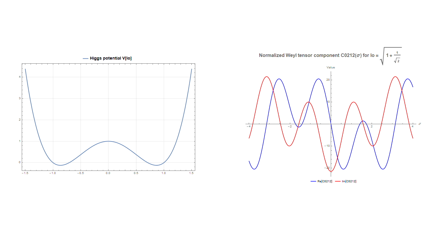
where V is the classical Higgs potential and the broken symmetry in the system can be interpreted as an apparent mismatch of coefficients related to . The Figure 1 shows the classic "Mexican sombrero" potential . Since is related in equation (64) to the angle describing the spin, this means that in this solution the spin effect of the field is described by invariant angle (depends only on ) and, according to (83) it is closely related to the trace of the metric and, consequently, to the Ricci scalar in the curvilinear description and thus to spacetime curvature. This also at least means that to obtain correct results in curved spacetime in the Alena Tensor model, the Higgs-like potential is needed.
Since this paper considers a system with only electromagnetic field, the above described broken symmetry should be considered more as a consequence of the Higgs field in electromagnetism (equivalent to the Abelian mechanism and broken U(1) symmetry) visible in the curvilinear description within GR. However, the above result may contribute to a better understanding of the description of the Higgs field action within the GR containing electromagnetism and connections of the Higgs potential with curvature and spin seen in obtained result. Perhaps it will also help to extend Alena Tensor description to the electroweak field, which will allow to compare the quantum and curvilinear images, which, however, deserves a separate article.
For the whole metric becomes significantly simplified and symmetric
which means that it may be assumed that adopting the above value leads to some significant and physically important solution of the equations for the system.
Using hyperbolic identities and expressing
then using (59) one obtains
which allows for further analysis of the Higgs potential. For example, using (63) and (68), the relation between electromagnetic energy density , angle and spin four-vector zero component is therefore
Above also explains the origin of and the connection of spin and Lagrangian with the energy density of the electromagnetic field. Since, according to the considered Alena Tensor approach, in curved spacetime the energy density expressed by must vanish (the entire stress-energy tensor of the electromagnetic field vanishes), this means, that and thus in curved spacetime becomes invariant, which allows to analyze the transition to curved spacetime.
One may now consider what value the Alena Tensor takes in curved spacetime. To do this, it is easiest to analyze the behavior of . As one may calculate, the determinant of this tensor is 0 and the matrix rank is 2, but, as described in the introduction, it degenerates to in curved spacetime. It can be seen that in the Alena Tensor approach the metric follows from propagation. However, in curved spacetime the electromagnetic field according to this approach should vanish, remaining present only in the metric and determining geodetic. This can be achieved by degenerating vectors and to a single vector in curved spacetime . However, in such situation the equation (71) forces this vector to be the four-velocity, divided by the Lorenz factor
which degenerates from (73) to the form
As can be easily verified, the exact above relation of variables leads to the vanishing field stress-energy tensor in (75) upon transition to curved spacetime.
Since the metric is known and may be expressed by values of , in flat spacetime thanks to (71) this allows to easy obtain the normalized Einstein tensor and Ricci tensor (normalized by ) using the equation (19). According to the notation used in (19) one obtains
where Ricci scalar R (normalized according to notation used) may be calculated as .
The described system seems to be Petrov type D or II [35], although to be sure, the Weyl tensor should be calculated. This does not seem possible for the general case (without auxiliary assumptions about symmetries), but one could simplify the obtained description considerably, based on the following observation. One may notice, that the vanishing Lorentz factor in can be interpreted as an important suggestion for the description of motion in curved spacetime. Such motion would correspond to a stream of particles moving without dilation, a strictly ordered flow without local perturbations, resembling a perfect, infinitely stiff fluid. This means that should be the Killing tensor and the system should have hidden symmetry (similar to the Carter constant in Kerr solutions).
As shown previously, product of the basis is in considered case , which means that null vectors have global significance for spacetime geometry, thus Killing tensor should have a strong connection with propagation along null vectors (it is not a random symmetry, but a deep feature of spacetime) and this would mean the existence of special wave surfaces, e.g. electromagnetic waves and/or gravitational radiation. This would be also a clear indication that spacetime belongs to the Petrov D or II class and is associated with wave propagation solutions.
Also, the analysis of obtained equations drive to conclusion, that energy (energy density) is not something external to geometry in Alena Tensor approach, but energy is defined by the geometry of spacetime itself. This is a result in the spirit of General Relativity, but it goes even deeper: metric depends on , but at the same time depends on the metric because it is trace of in this metric. The system itself defines its own energy through the structure of the field, which is similar to the idea of Self-consistent Field [36] - where the field and the source are inseparable, or Emergent Gravity [37,38] - where energy, gravity and geometry arise from a common structure, or Induced Geometry [39] - where energy comes from deformation of spacetime itself, as e.g. in Sakharov’s theory [40]. It seems impossible to "decree" energy in Alena Tensor, but it must be calculated from geometry and the system works as a closed causal cycle.
The dependence for of its norm and trace in curved spacetime (the norm is the square of the trace) is a key property for null space and suggests that describes isometries related to null wave propagation, similar to pp-wave [41] and Robinson-Trautman solutions [42], what is actually expected in considered approach based on electromagnetic stress-energy tensor and result (79). This would also mean that the Killing tensor is directly related to the energy distribution in spacetime as expected, similar to other GR solutions (eg. Kerr solution), and lead to a rather groundbreaking but also expected result in the context of the discussed approach, that the Killing tensor directly determines the Einstein tensor in main GR equation.
Since is simply the Alena Tensor (stress-energy tensor for the system) divided by , it gives correct conserved values in the Noether formalism (conserved density of energy and momentum). From the definition of the Alena Tensor as the energy-momentum tensor for the system it also follows that is symmetric and vanishes.
Since this implies that along a geodesic parametrized by proper time , its total derivative vanishes.
Using the symmetry of one may note that
Therefore, the condition
holds for arbitrary tangent vectors , and it indeed follows that . Therefore normalized Alena Tensor is Killing tensor for considered system.
In this way Alena Tensor theory, in curved spacetime, becomes equivalent to some specific case of General Relativity equation expressed in the following form
where according to (19) in the above equation is the classical Einstein tensor in commonly used notation (classical Einstein tensor) and (cosmological constant).
Thanks to the above, since the Weyl tensor is defined as the part of the Riemann tensor that does not depend on the Ricci tensor, this implies that since Killing tensor determines the Einstein tensor, and the Einstein tensor determines the Ricci tensor, then one could calculate the Weyl tensor by extracting the part of the curvature that does not contain the Ricci tensor. This would also mean that the Christoffel symbols can be expressed as a function of the Killing and Einstein tensors, and the Riemann tensor can be written directly as a function of the Ricci and Killing tensors.
For the considered system with only electromagnetism (two null vectors in metric), one may therefore construct a general Weyl tensor ansatz , which must contain only components that do not become zero when the trace part is subtracted from the Riemann tensor. It should be of the form
where
It is easy to check that the above tensors are linearly independent and form the basis for the representation of any Weyl tensor in the system under consideration. Analysis of their behavior indicates that
- is responsible for "pure" directional propagation, e.g. a gravitational wave propagating along null directions (purely conformal part of the Weyl tensor, described solely by null geometry),
- describes non-radiating, "axial" deformation of space, e.g. tidal sequences, consistent with mass motion without undulations,
- describes conformal distortion of the background metric itself.
The coefficients , , are not known a priori, but one may determine them with help of Riemann tensor. To obtain Riemann tensor in the system under consideration, it is enough to assume the following ansatz
It has the following justification
- The Riemann tensor satisfies the known algebraic symmetries: . The above ansatz satisfies them automatically.
- There are only two tensor objects available in the system: the metric and the Killing tensor . The Riemann tensor must be constructed exclusively from them.
- The first term with corresponds to the geometry of a spacetime with constant curvature, as in de Sitter spacetime:
- The second term with is the minimal geometrically correct extension that takes into account the presence of non-null energy (represented by ). Its construction provides correct symmetries and enables the reproduction of a non-null Ricci tensor
- Other possible combinations (e.g. ) are linearly dependent or asymmetric with respect to the required properties of the Riemann tensor, and do not provide new information in the case under consideration.
- The whole creates the most general fourth-order tensor with Riemann symmetries, which can be constructed from available geometric objects.
Computing the contraction of the above Riemann tensor anstaz with one gets
Since normalized Ricci tensor is known (93), therefore considering for simplicity above Riemann tensor anstaz as normalized, one gets
Such normalized form is convenient to use because it allows one to easily obtain both: classical tensors (multiplication by the cosmological constant ) and tensors in the Alena Tensor notation (multiplication by field invariant ).
Next, one may consider normalized trace part of the Riemann tensor , which provides the necessary symmetries and the vanishing trace in the Weyl tensor. For this to be satisfied, trace part must have the following, classical [43] form (where Ricci tensor is considered for simplicity also as normalized):
Since all terms related to reduce after grouping the components in , one obtains normalized Weyl tensor in generalized form for the system under consideration
Trace of above Weyl tensor disappears and it has all the expected symmetries. Substituting the metric known from (79), one obtains the coefficients postulated in the anstaz (98) and as one may notice from non-zero coefficient , gravitational waves exist in the system.
One can also demonstrate the existence of gravitational waves using classical analysis using the Weyl tensor components and Newman-Penrose formalism [44]. Having calculated the above-mentioned tensors and sample basis (78), one may notice, that four-vector is purely real. One may thus construct a Newman-Penrose tetrad around it, fitting to the geometry of the system, as follows
The above four-vectors satisfy all the tetrad requirements and lead to only two non-zero NP scalars
what is confirmed in the supplementary materials. Scalar can be zeroed by a rotation around without modifying and the system under consideration with sample is thus Petrov type III or N. However, taking into account the non-zero Ricci tensor and the Bel criteria, considered spacetime must be Petrov type III, since due is built from reversible metric (111), thus there does not exist any vector satisfying .
Therefore, finally, spacetime described by Alena Tensor with only electromagnetic field may be interpreted as a certain form of the Kundt solution with dust [45] and for sample it is Petrov type III, similar to described in [46,47]. One may also notice, that additional fields added to the Alena Tensor depending on the new null directions should break the obtained degeneracy leading to the general Petrov type I case.
One may also substitute an example basis (78) into Weyl tensor to analyze its values. Table 1 presents the values of the key components of the Weyl tensor in this basis.

Table 1.
Component values of the Weyl tensor.
| Component | Value |
|---|---|
| 0 | |
| 0 | |
| 0 | |
| 0 |
One may then solve the system of equations (59, 77, 86) presenting the results only as a function of and . Due to the complex relationships between variables, analytical solution and obtained results are presented in supplementary file. Weyl tensor component values were calculated for the value adopted for the analysis (87) and for chosen solution . The Figure 2 below clearly shows the wave nature of the component of the Weyl tensor, presenting the result of the calculations performed. Obtained Weyl tensor component seems to encode the variation of some curvature field along the propagating direction .
Gravitational waves are often modeled using Gaussian impulse as in [48], but this can also be done using the dependence of on . One may therefore show in Figure 3 the deformation effects for an example arrangement of test particles on a circle. In the supplementary materials there are calculations and a gif file presenting animation of this distortion. This animation reveals the typical quadrupolar nature of spacetime distortions induced by gravitational waves (characteristic twisting and stretching).
The above Weyl tensor components are actually normalized. One may thus present the main GR equation in the Alena Tensor notation (19) and represent it using the vacuum pressure as follows
Since the obtained Weyl tensor is normalized (by ) this means that the interpretation from (42) that gravitational waves in the Alena Tensor approach are in fact propagating vacuum pressure disturbances also seems to be correct.
It is also worth noting that the obtained metric term can in principle be interpreted as a vacuum energy contribution (effective cosmological constant) as in [49,50] playing the role of a metric scaling factor, as e.g. described in [51].
The gravitational waves discussed here represent a simplified case for the electromagnetic field and gravity and require generalization to all fields. However, it is possible to reason about more general solutions without knowing the full metric.
3.3. Effective Description of Gravity for the General Case
One may invoke the scalar field associated with the presence of matter, where . It is known from Section 2.2 that is responsible for the presence of sources and in their absence . Therefore, interpreting whole as the wave amplitude tensor one would get representation which would also allow to search for as a certain wave function.
This approach allows for a simplification related to the analysis of gravitational waves. Considering the force responsible for effects related to gravity as shown in (24) and extracting the acceleration from it, one gets
since according amendment from [11] .
As shown in [10], is directly related to the effective potential in gravitational systems which can be calculated from the GR equations. This would allow searching for propagating changes of the effective potential itself () similarly as was postulated in [52]. It would significantly simplify both the calculations and perhaps the methods of detecting gravitational waves, for example, using the approach discussed in [53].
It may therefore be assumed, that the field is related to the effective potential or e.g. timelike component of the metric used for curvilinear description of the system by
that is, plays the role of a local gravitational potential in the sense of effective geometry. As has been repeatedly demonstrated previously, for such a defined potential (assuming, for example, the Schwarzschild potential) [54], the correct effects are obtained regarding light path curvature, Mercury’s perihelion precession or the Shapiro effect. However, the energy radiated by gravitational waves requires further discussion.
The above potential can be extended to gravito-electromagnetic (GEM) four-potential in the form according to the approach presented e.g. in [55]. The most general form of the gravitomagnetic vector potential in the present formalism can be written as a multipolar expansion of the current-type source moments, fully analogous to the electromagnetic case
where
- is the retarded time, ensuring causal propagation of the field from the source to the observer
- are the current-type multipole moments of the source (), directly related to the mass-current distribution inside the source They encode the full time dependence of the gravitomagnetic field, including both stationary and radiative contributions
- are the toroidal vector spherical harmonics on the unit sphere, representing the purely rotational (divergence-free) part of the vector field on
- corresponds to the spin-dipole (total angular momentum vector ), which dominates in the far zone for an isolated rotating body
- are the higher current multipoles, describing more complex rotational structures of the source (e.g. internal circulation, non-axisymmetric rotation)
Within the GEM formalism, the fields follow from
and contains the complete information about the "electric" and "magnetic" parts of the Weyl tensor
This guarantees that for arbitrary and , one may reproduce any radiative Weyl tensor compatible with the Einstein equations in the linear regime. Most authors in this context adopt the classical Maxwellian analogy, developing the gravitomagnetic description in the linear frame [56,57,58,59]. Others rely on the Weylian approach, formulating the GEM directly from the curvature tensor or proposing its extensions and generalizations [60,61,62,63]. However, this classical reasoning can be modified, obtaining the correct GEM description for gravitational waves.
For the scalar sector one may introduce a 4D symmetric trace-free Hessian (“electric tidal precursor”)
and introduce projector as
For the vector sector one may introduce a 4D “magnetic tidal precursor” by first forming the observer-relative gravitomagnetic vector
and then take its symmetric trace-free spatial gradient
Removing the spatial trace as above, one may define the total tidal precursor
Let be a unit spacelike vector orthogonal to in the far zone and
The TT gravitational-wave field sourced by the four-potential is then
where is the characteristic angular frequency and is a (common) multipole-dependent normalization, fixed by matching the total radiated power to GR multipole results (so that the scalar and current-type sectors radiate with the standard strength).
Choosing an orthonormal basis on the screen with , one may set
and define the polarizations
so that . The Isaacson effective tensor then yields, in the rest frame
For a monochromatic far-zone mode the TT projection vanishes for , while for
where and are, respectively, the scalar (mass-type) and current-type multipolar amplitudes entering and . One may now compare the above to the scalar far-zone flux from Peters-Matthews formula [64], treating this result as the expected emission power. By reconciling the result, one obtains
This normalization ensures exact agreement in description of gravitational waves for , while modes carry no TT tensor radiation.
In the far zone, one may equivalently reconstruct the metric perturbation in the TT gauge from the four-potential-built field by setting, as in (82)
Computing the Weyl tensor from this metric yields
which coincides with the Newman-Penrose description used to fix .
The normalized Weyl from (111) is related to the physical curvature by , so that projecting this Weyl tensor onto a Minkowski tetrad gives
Here, is the geometric scale relating the normalized tensor to the metric-derived curvature. With defined from the source multipoles, the scalar-vector formalism reproduces the full radiative content of GR while retaining a simplified structure for practical computations, in which the "electric” and "magnetic” parts of the Weyl tensor follow directly from the four-potential.
Importantly, it can be calculated that the above reasoning significantly simplifies the calculations of gravitational waves also for known metrics, e.g. the Kerr metric. Considering the stationary Kerr solution itself, the four-potential is time-independent, so that , and the tidal precursors and contain only static near-zone terms that vanish after the TT projection. One therefore finds and , in full agreement with the fact that the Kerr geometry (Petrov type D) carries no radiation.
Considering instead a small time-dependent quadrupolar perturbation on the Kerr background, the formalism reproduces the standard quadrupole emission power of general relativity: for modes
while all contributions vanish, consistently with the spin-2 character of the gravitational field. This confirms that the scalar-vector construction not only suppresses spurious radiation for stationary spacetimes, but also yields the correct leading-order gravitational-wave power for perturbed Kerr sources.
4. Conclusion and Discussion
As shown in the above article, the Alena Tensor ensures the existence of gravitational waves and allows their physical interpretation, providing key tools for their further analysis including the ability to calculate and visualize Weyl tensor components. The obtained decomposition of the electromagnetic field stress-energy tensor (79) allows for further analysis of metrics for curved spacetimes (e.g. extending obtained solution for other fields) and also to use the proposed null basis for further Alena Tensor development in the framework of conformal geometry, the NP formalism and the description of photons in QFT. It also seems reasonable to generalize above results for all known fields or to non-linear electromagnetism (using e.g. approach presented in [65]) and search for a description of elementary particles that could provide relatively stable solutions to the obtained equations, perhaps also taking into account new approaches, such as those proposed in [66]. A discussion of the main conclusions of the article is grouped into three key sections below.
4.1. Conclusions About GR and Gravitational Waves
As this article clearly shows, Alena Tensor narrows the class of available GR solutions. In this mathematical framework
- The cosmological constant is indeed constant in curved spacetime.
- The energy-momentum tensor of the system in curved spacetime becomes the Killing tensor.
- The available metrics take on a specific form (2+ null vectors and a background metric). Although the paper presents the metric only for a system with electromagnetism and gravity, the Alena Tensor model enforces this metric arrangement in general case.
- The resulting Riemann tensor describes the general case, ensures the formation of the Ricci tensor in contraction, and allows for the derivation of the Weyl tensor.
It is worth noting that the obtained non-zero form of the normalized Weyl tensor (111) built on the basis of the metric tensor used for curvilinear description, given as will not change regardless of the fields considered and no matter how many null vectors the metric consists of (assuming more complex fields than electromagnetism). This Weyl tensor has also an important property: for any tetrad considered in curved spacetime, all NP scalars become zero, and they remain non-zero only for tetrads constructed on the background Minkowski metric. This means that gravitational waves derived from Alena Tensor are undetectable for curvilinear observers in their local frame of reference and can be detected only against the background of the Minkowski metric. Therefore, according to the postulate (41), gravitational waves are not "local fluctuations" of curvature but global effects of the difference of geometry with respect to a flat background, similar to postulated in [67,68]. This result has a rather intuitive interpretation and means that, according to the equivalence principle, observers in curved spacetime do not experience gravity in any form, including gravitational waves, because their tetrad "co-curves" with the geometry.
The obtained form of the Weyl tensor can thus be treated as a formal geometry of the equivalence principle and as a requirement for every physically possible solution of GR, which would, however, require a separate proof. This direction of further research also seems very important, because it would provide a formal justification for the fact that the measurability of gravity is relational, not absolute, and also offers a new way of considering quantum gravity: not so much as field fluctuations, but as fluctuations of the geometric background with respect to the algebraically defined Weyl tensor. This result is of particular importance e.g. in the context of Penrose’s Weyl curvature hypothesis [69], developed in e.g. [70,71]. The discussion about what gravity is [72] remains open, and Alena Tensor joins this discussion.
The connection between Alena Tensor and the Killing tensor obtained in this paper reveals a deep, nonlinear connection between the matter distribution and the geometry and symmetries of spacetime. These results show that the matter distribution in this approach is not arbitrary, but precisely tuned to the geometry and hidden symmetries of spacetime, which allows for their further analysis in the language of Killing tensors and conformal Weyl curvature. This also explains why in flat spacetime is Noether tensor and in curved spacetime, tensor turns into the Killing tensor, requesting, that translational symmetries in turn into isometries of Killing vectors in .
The obtained results regarding gravitational waves are qualitative in nature, as it is difficult to provide quantitative experimental verification for sources understood as a consequence of the existence of an electromagnetic field alone. The Alena Tensor model, unlike other models, links the GR results to the fields under consideration, treating matter solely as a consequence of the fields’ existence. This requires extending the model to all gauge fields to make realistic predictions, since generalization of the Alena Tensor to other fields (e.g. electroweak) may correct some results, providing the possibility of experimental verification of the predictions for more realistic sources. However, certain conclusions can be drawn that may allow experimental verification of the obtained results.
The obtained picture of Kundt spacetime with dust would suggest, that in gravitational waves for sources that can be treated simplistically as the result of the existence of an electromagnetic field alone, one should be able to observe effects related to non-zero (visible twisted components). The obtained x and + polarizations resulting from the Weyl tensor values (121) are consistent with the general conclusions of GR and LIGO/Virgo data [73]. Because the waveform depends strictly on the source dynamics, it cannot be analyzed without additional assumptions about the sources introduced into the metric. This does not seem possible directly for such simplified sources as those discussed here and requires generalization of the Alena Tensor to other gauge fields.
However, as shown in Section 3.3, one can describe effective gravity for general case based on the Alena Tensor approach, which provides an accurate representation of the energy radiated by the system for all multipoles, while remaining in full agreement with GR results. This approach allows for a radical simplification of the calculation of gravitational waves also for known metrics (e.g. Kerr metric) while confirming the correctness of the GEM approach. The construction of the field and the effective stress-energy tensor reproduces, at leading order in the far zone, the full angular power distribution of GR gravitational radiation for each individual mode with , including the standard quadrupolar pattern for . After the proper amplitude identification , the total emitted power and its multipolar decomposition match exactly the GR results, where modes produce no TT radiation, in agreement with the spin-2 character of the field.
Moreover, in the radiative far zone one may equivalently reconstruct the metric perturbation in TT gauge with a constant conformal factor in a Kerr-Schild-type ansatz, and compute the physical Weyl tensor. This establishes a direct equivalence between the scalar-field formalism and the metric/Weyl description of gravitational radiation, and identifies as the geometric curvature scale linking the normalized Weyl tensor to the physical spacetime curvature, without altering any observable far-zone quantities. The obtained correct emission powers also impose the conclusion that the description of motion in the gravitational field, waveforms, and dispersion resulting from the Alena Tensor schould also correspond to the results obtained in GR, although, of course, this is still worth confirming with separate calculations.
4.2. Possible Directions of Further Unification
As discussed in Section 2.3, the Alena Tensor could be generalized to all gauge fields, but this requires further research. The research on gravity and electromagnetism carried out in this article according to the approach of Alena Tensor shows that, surprisingly, it naturally forces the existence of the Higgs-like potential and this potential turns out to be necessary to even consider curved spacetime. The spontaneously appearing faithful reproduction of the Higgs potential may of course be a completely coincidental result, but it may also be an indication that the proposed approach is worth further investigation and development for other fields (electroweak, strong or more general solutions), to obtain complete picture of unification.
This direction of research seems to be particularly important. For example, the unification of gravity with electroweak interactions has been analyzed so far, among others, in the context of symmetry breaking and gauge geometry [74,75], through the prism of the influence of gravity on the global properties of quantum vacuum [76,77], analogies between spin-gravity coupling and the Higgs mechanism [78] or analysis of chiral fermions and CPT symmetry in the presence of curvature [79,80]. It seems that the approach considered in the article best fits into the last of these research directions, due to the possibility of analyzing the structure of the Weyl curvature, the potential asymmetry of gravitational waves (related to ) and because it actually touches upon chirality in the spatial and propagation sense, although not directly in the fermion sense.
An equally interesting research direction seems to be the use of the smooth transition between classical, quantum and curvilinear descriptions provided by the Alena Tensor to reanalyze existing studies, such as [81].
4.3. Conclusions on Energy Conservation in Energy-Momentum Tensors
It is also worth raising the issue of the energy conservation in the Alena Tensor. As it follows from chapter Section 2, this approach ensures local conservation of energy and momentum, because the four-divergence of the tensor describing matter cancels the four-divergence of the field tensors. Additionally, for electromagnetism, the Alena Tensor turned out to be a symmetric, canonical Noether tensor with vanishing four-divergence. A similar result can be expected after extending the Alena Tensor to all gauge fields, because this approach provides a conclusion, that the cosmological constant is actually constant, which strengthens the argument for conservation of energy. Although, obviously, another scenario should also be considered, especially in the context of the dark sector.
It was e.g. shown in [82] that violating conservation of energy can generate effects corresponding to dark energy, making such approaches attractive for cosmology. Similarly, in scalar-tensor theories in the Einstein framework [83], the coupling of the dilaton to matter causes energy not to be conserved locally, justifying a reinterpretation of the field as effective. Also approaches based on non-commutative structures, such as [84], introduce non-classical position operators, which result in four-momentum fluctuations and energy can transfer between geometric dimensions, formally manifested as a nonzero divergence of the energy-momentum tensor.
As shown in [85], many nonconservative theories rely on geometric coupling, e.g., or a modified metric structure, resulting in . In particular, Rastall theory [86,87] introduces a dependence of the four-divergence on the gradient of the Ricci scalar , resulting in effective energy creation or annihilation depending on the local curvature. This approach enables flexible modeling of dark energy and dark matter, and therefore provides a better fit to cosmological data. Violating the energy conservation principle while maintaining the metric, modifies the behavior of matter, but does not generate causality violations and ensures formal convergence with effective and entropy theories.
In diffusion models [88], the describe entropy fluctuations, enabling consideration of thermodynamic mechanisms of energy flow. Similar mechanisms occur in wave collapse theories in quantum mechanics [89], where random perturbations to the system’s state lead to a constant exchange of energy with the background. Thanks to such approach, violation of local conservation of energy and momentum is not an artifact of a flawed theory, but a deliberate extension of the classical framework, leading to new conclusions about the nature of energy, gravity, and cosmological evolution.
In [90] a wide class of modified gravity theories is discussed, including scalar-tensor or theories, where additional geometric components coupled to matter appear. In many models, the matter divergence is locally nonzero, but by influencing the metric it is possible to conserve some form of global energy in an effective sense, and global boundary conditions (e.g., asymptotic flatness) determine whether a total conserved energy can be defined. E.g., the model described in [91] is based on the general relativistic thermodynamics equation (Gibbs-Duhem) and allows for fluctuations in entropy, temperature, and interactions. The lack of local conservation thus translates into a global impact: thermodynamic actions can model dark energy and the expansion of the Universe. An important consequence is that total energy is not conserved globally, which has key cosmological implications, e.g., extending the age of the Universe through non-conservative dynamics.
Also in the context of unimodular gravity, the authors show that a local violation of a conservation law, even a very small one, can generate the effect of an effective cosmological constant. If energy is not conserved locally, a global effect (e.g., a positive accelerating influence) can be interpreted as a source of dark energy, directly linking local divergence to global cosmological observations.
In light of the above review, in addition to generalizing to other fields, it is worth considering a potential modifications of the Alena Tensor, adapting it to non-conserved energy-momentum frameworks. This would open up additional possibilities for analyzing non-classical solutions and new directions of reasoning contained in these publications, which could also increase the unification potential of the Alena Tensor.
In conclusion, it remains an open question whether the Alena Tensor is a correct way to describe physical systems, but this paper shows that it exhibits many properties that are expected from such a description, including the existence of gravitational waves whose behavior and description agrees with GR. The author hopes that the results obtained in this article will facilitate further use of discussed approach as a tool that can help develop many different concepts. It seems that its further analysis may provide useful descriptions of the transformation between curved and flat spacetime and bring new insights that will contribute to a better understanding of issues related to the broadly understood unification of physical theories.
Supplementary Materials
The following supporting information can be downloaded at the website of this paper posted on Preprints.org.
Funding
Author did not receive support from any organization for the submitted work. Author have no relevant financial or non-financial interests to disclose.
Data Availability Statement
All data that support the findings of this study are included within the article (and any supplementary files).
Acknowledgments
During the preparation of this work the author did not use generative AI or AI-assisted technologies.
References
- Bailes, M.; Berger, B.K.; Brady, P.; Branchesi, M.; Danzmann, K.; Evans, M.; Holley-Bockelmann, K.; Iyer, B.; Kajita, T.; Katsanevas, S.; et al. Gravitational-wave physics and astronomy in the 2020s and 2030s. Nature Reviews Physics 2021, 3, 344–366. [Google Scholar] [CrossRef]
- Schutz, B.F. Gravitational wave astronomy. Classical and Quantum Gravity 1999, 16, A131. [Google Scholar] [CrossRef]
- Bernardo, R.C.; Ng, K.W. Charting the nanohertz gravitational wave sky with pulsar timing arrays. International Journal of Modern Physics D 2025, 34, 2540013. [Google Scholar] [CrossRef]
- Grant, A.M.; Nichols, D.A. Outlook for detecting the gravitational-wave displacement and spin memory effects with current and future gravitational-wave detectors. Physical Review D 2023, 107, 064056. [Google Scholar] [CrossRef]
- Borhanian, S.; Sathyaprakash, B. Listening to the universe with next generation ground-based gravitational-wave detectors. Physical Review D 2024, 110, 083040. [Google Scholar] [CrossRef]
- Milgrom, M. Gravitational waves in bimetric MOND. Physical Review D 2014, 89, 024027. [Google Scholar] [CrossRef]
- Tahura, S.; Nichols, D.A.; Yagi, K. Gravitational-wave memory effects in Brans-Dicke theory: Waveforms and effects in the post-Newtonian approximation. Physical Review D 2021, 104, 104010. [Google Scholar] [CrossRef]
- Matos, I.S.; Calvão, M.O.; Waga, I. Gravitational wave propagation in f (R) models: New parametrizations and observational constraints. Physical Review D 2021, 103, 104059. [Google Scholar] [CrossRef]
- Shapiro, I.L.; Pelinson, A.M.; de, O. Salles, F. Gravitational waves and perspectives for quantum gravity. Modern Physics Letters A 2014, 29, 1430034. [Google Scholar] [CrossRef]
- Ogonowski, P.; Skindzier, P. Alena Tensor in unification applications. Physica Scripta 2024, 100, 015018. [Google Scholar] [CrossRef]
- Ogonowski, P. Proposed method of combining continuum mechanics with Einstein Field Equations. International Journal of Modern Physics D 2023, 2350010, 15. [Google Scholar] [CrossRef]
- Ogonowski, P. Developed method: interactions and their quantum picture. Frontiers in Physics 2023, 11, 1264925. [Google Scholar] [CrossRef]
- Logunov, A.; Mestvirishvili, M. Hilbert’s causality principle and equations of general relativity exclude the possibility of black hole formation. Theoretical and Mathematical Physics 2012, 170, 413. [Google Scholar] [CrossRef]
- Friedman, Y. Superposition principle in relativistic gravity. Physica Scripta 2024, 99, 105045. [Google Scholar] [CrossRef]
- Poplawski, N.J. Geometrical formulation of classical electromagnetism. arXiv 2008, arXiv:0802.4453. [Google Scholar] [CrossRef]
- Chang, Y.F. Unification of gravitational and electromagnetic fields in Riemannian geometry. arXiv 2009, arXiv:0901.0201. [Google Scholar] [CrossRef]
- Chernitskii, A. On unification of gravitation and electromagnetism in the framework of a general-relativistic approach. Gravitation and Cosmology 2009, 15, 151–153. [Google Scholar] [CrossRef]
- Kholmetskii, A.; Missevitch, O.; Yarman, T. Generalized electromagnetic energy-momentum tensor and scalar curvature of space at the location of charged particle. arXiv 2011, arXiv:1111.2500. [Google Scholar] [CrossRef]
- Novello, M.; Falciano, F.; Goulart, E. Electromagnetic Geometry. arXiv 2011, arXiv:1111.2631. [Google Scholar] [CrossRef]
- de Araujo Duarte, C. The classical geometrization of the electromagnetism. International Journal of Geometric Methods in Modern Physics 2015, 12, 1560022. [Google Scholar] [CrossRef]
- Hojman, S.A. Geometrical unification of gravitation and electromagnetism. The European Physical Journal Plus 2019, 134, 526. [Google Scholar] [CrossRef]
- Woodside, R. Space-time curvature of classical electromagnetism. arXiv preprint gr-qc/0410043 2004. [Google Scholar] [CrossRef]
- Bray, H.; Hamm, B.; Hirsch, S.; Wheeler, J.; Zhang, Y. Flatly foliated relativity. arXiv preprint arXiv:1911.00967 2019, arXiv:1911.00967 2019. [Google Scholar] [CrossRef]
- Jafari, N. Evolution of the concept of the curvature in the momentum space. arXiv preprint arXiv:2404.08553 2024, arXiv:2404.08553 2024. [Google Scholar] [CrossRef]
- Kaur, L.; Wazwaz, A.M. Similarity solutions of field equations with an electromagnetic stress tensor as source. Rom. Rep. Phys 2018, 70, 1–12. [Google Scholar]
- MacKay, R.; Rourke, C. Natural observer fields and redshift. J Cosmology 2011, 15, 6079–6099. [Google Scholar]
- Ahmadi, N.; Nouri-Zonoz, M. Massive spinor fields in flat spacetimes with nontrivial topology. Physical Review D—Particles, Fields, Gravitation, and Cosmology 2005, 71, 104012. [Google Scholar] [CrossRef]
- Waluk, P.; Jezierski, J. Gauge-invariant description of weak gravitational field on a spherically symmetric background with cosmological constant. Classical and Quantum Gravity 2019, 36, 215006. [Google Scholar] [CrossRef]
- Shen, J.Y.; Peng, C.; Li, L.X. Multiway Junction Conditions for Spacetimes with Multiple Boundaries. Phys. Rev. Lett. 2024, 133, 131601. [Google Scholar] [CrossRef]
- Czech, B.; Lamprou, L.; McCandlish, S.; Sully, J. Integral geometry and holography. Journal of High Energy Physics 2015, 2015, 1–41. [Google Scholar] [CrossRef]
- Forger, M.; Römer, H. Currents and the energy-momentum tensor in classical field theory: a fresh look at an old problem. Annals of Physics 2004, 309, 306–389. [Google Scholar] [CrossRef]
- Blaschke, D.N.; Gieres, F.; Reboud, M.; Schweda, M. The energy-momentum tensor(s) in classical gauge theories. Nuclear Physics B 2016, 912, 192–223. [Google Scholar] [CrossRef]
- Kosyakov, B. Self-interaction in classical gauge theories and gravitation. Physics Reports 2019, 812, 1–55. [Google Scholar] [CrossRef]
- Anghinoni, B.; Flizikowski, G.; Malacarne, L.C.; Partanen, M.; Bialkowski, S.; Astrath, N.G.C. On the formulations of the electromagnetic stress-energy tensor. Annals of Physics 2022, 443, 169004. [Google Scholar] [CrossRef]
- Hall, G. Wave Surface Symmetry and Petrov Types in General Relativity. Symmetry 2024, 16, 230. [Google Scholar] [CrossRef]
- Ignat’ev, Y.G. The self-consistent field method and the macroscopic universe consisting of a fluid and black holes. Gravitation and Cosmology 2019, 25, 354–361. [Google Scholar] [CrossRef]
- Padmanabhan, T. Emergent gravity paradigm: recent progress. Modern Physics Letters A 2015, 30, 1540007. [Google Scholar] [CrossRef]
- Volovik, G. Fermi-point scenario for emergent gravity. arXiv preprint arXiv:0709.1258 2007, arXiv:0709.1258 2007. [Google Scholar] [CrossRef]
- Eichhorn, A.; Surya, S.; Versteegen, F. Induced spatial geometry from causal structure. Classical and Quantum Gravity 2019, 36, 105005. [Google Scholar] [CrossRef]
- Sakharov, A.D. Vacuum quantum fluctuations in curved space and the theory of gravitation. General Relativity and Gravitation 2000, 32, 365–367. [Google Scholar] [CrossRef]
- Sämann, C.; Steinbauer, R.; Švarc, R. Completeness of general pp-wave spacetimes and their impulsive limit. Classical and Quantum Gravity 2016, 33, 215006. [Google Scholar] [CrossRef]
- Davidson, W. Robinson-Trautman solutions to Einstein’s equations. General Relativity and Gravitation 2017, 49, 1–4. [Google Scholar] [CrossRef]
- Stavrov, I. Curvature of space and time, with an introduction to geometric analysis; Vol. 93, American Mathematical Soc., 2020.
- Jizba, P.; Mudruňka, K. Newman-Penrose formalism and exact vacuum solutions to conformal Weyl gravity. Physical Review D 2024, 110, 124006. [Google Scholar] [CrossRef]
- Fuster Pérez, A. Kundt spacetimes in general relativity and supergravity. PhD thesis, Vrije U., Amsterdam, 2007.
- Kuchynka, M.; Pravdová, A. Weyl type N solutions with null electromagnetic fields in the Einstein-Maxwell p-form theory. General Relativity and Gravitation 2017, 49, 1–13. [Google Scholar] [CrossRef]
- Hervik, S.; Ortaggio, M.; Pravda, V. Universal electromagnetic fields. Classical and Quantum Gravity 2018, 35, 175017. [Google Scholar] [CrossRef]
- Datta, S.; Guha, S. Memory effect of gravitational wave pulses in PP-wave spacetimes. Physica Scripta 2024, 99, 075023. [Google Scholar] [CrossRef]
- Wang, Q. Reformulation of the cosmological constant problem. Physical Review Letters 2020, 125, 051301. [Google Scholar] [CrossRef]
- Gueorguiev, V.G.; Maeder, A. Revisiting the Cosmological Constant Problem within Quantum Cosmology. Universe 2020, 6, 108. [Google Scholar] [CrossRef]
- Marsh, A. Defining geometric gauge theory to accommodate particles, continua, and fields. Journal of Mathematical Physics 2024, 65. [Google Scholar] [CrossRef]
- Domènech, G. Scalar induced gravitational waves review. Universe 2021, 7, 398. [Google Scholar] [CrossRef]
- Athron, P.; Balázs, C.; Fowlie, A.; Morris, L.; Searle, W.; Xiao, Y.; Zhang, Y. PhaseTracer2: from the effective potential to gravitational waves. The European Physical Journal C 2025, 85, 1–35. [Google Scholar] [CrossRef]
- Vossos, S.; Vossos, E.; Massouros, C.G. The Relation between General Relativity’s Metrics and Special Relativity’s Gravitational Scalar Generalized Potentials and Case Studies on the Schwarzschild Metric, Teleparallel Gravity, and Newtonian Potential. Particles 2021, 4, 536–576. [Google Scholar] [CrossRef]
- Maartens, R.; Bassett, B.A. Gravito-electromagnetism. Classical and Quantum Gravity 1998, 15, 705. [Google Scholar] [CrossRef]
- Ruggiero, M.L. A note on the gravitoelectromagnetic analogy. Universe 2021, 7, 451. [Google Scholar] [CrossRef]
- Bini, D.; Mashhoon, B.; Obukhov, Y.N. Gravitomagnetic helicity. Physical Review D 2022, 105, 064028. [Google Scholar] [CrossRef]
- Hao, D.; Hu, J.; Yu, H. Quantum gravitomagnetic interaction. Physical Review D 2024, 109, 126016. [Google Scholar] [CrossRef]
- Romano, A.E.; Vallejo-Peña, S.A. Gravitoelectromagnetic quadrirefringence. Physics of the Dark Universe 2024, 44, 101492. [Google Scholar] [CrossRef]
- Ramos, J.; de Montigny, M.; Khanna, F. Abelian and non-Abelian Weyl gravitoelectromagnetism. Annals of Physics 2020, 418, 168182. [Google Scholar] [CrossRef]
- Garza, A.; Luna, C.; Ramos, J. Retarded solutions for Weyl gravitoelectromagnetic fields. Canadian Journal of Physics 2023, 101, 358–362. [Google Scholar] [CrossRef]
- Ludwig, G.O. Extended gravitoelectromagnetism. I. Variational formulation. European Physical Journal Plus 2021, 136, 373. [Google Scholar] [CrossRef]
- Cáceres, E.; Kent, B.; Balaji, H.P. Gravito-electromagnetism, Kerr-Schild and Weyl double copies; a unified perspective. Journal of High Energy Physics 2025, 2025, 1–30. [Google Scholar] [CrossRef]
- Blanchet, L. Gravitational radiation from post-Newtonian sources and inspiralling compact binaries. Living reviews in relativity 2014, 17, 2. [Google Scholar] [CrossRef]
- Goulart, É.; Bergliaffa, S.E.P. Nonlinear electrodynamics nonminimally coupled to gravity: Symmetric-hyperbolicity and causal structure. APS, 2022, Vol. 105, p. 024021. [CrossRef]
- Rakitzis, T.P. Spatial wavefunctions of spin. Physica Scripta 2023. [Google Scholar] [CrossRef]
- Rovelli, C. Quantum Gravity; Cambridge University Press, 2004.
- Barbour, J. The End of Time: The Next Revolution in Our Understanding of the Universe; Oxford University Press, 1999.
- D’Amico, G.; Kaloper, N. Power-law inflation satisfies Penrose’s Weyl curvature hypothesis. Physical Review D 2022, 106, 103503. [Google Scholar] [CrossRef]
- Jizba, P.; Mudruňka, K. Newman-Penrose formalism and exact vacuum solutions to conformal Weyl gravity. Physical Review D 2024, 110, 124006. [Google Scholar] [CrossRef]
- Gregoris, D.; Ong, Y.C. Understanding gravitational entropy of black holes: a new proposal via curvature invariants. Physical Review D 2022, 105, 104017. [Google Scholar] [CrossRef]
- Capozziello, S.; De Falco, V.; Ferrara, C. Comparing equivalent gravities: common features and differences. The European Physical Journal C 2022, 82, 865. [Google Scholar] [CrossRef]
- Abbott, B.P.; Abbott, R.; Abbott, T.; Acernese, F.; Ackley, K.; Adams, C.; Adams, T.; Addesso, P.; Adhikari, R.X.; Adya, V.B.; et al. Tests of general relativity with GW170817. Physical review letters 2019, 123, 011102. [Google Scholar] [CrossRef]
- Alexander, S.; Alexandre, B.; Magueijo, J.; Pezzelle, M. Spontaneous Symmetry Breaking in Graviweak Theory. arXiv preprint arXiv:2505.17935 2025, arXiv:2505.17935 2025. [Google Scholar] [CrossRef]
- Shaposhnikov, M.; Shkerin, A.; Zell, S. Standard model meets gravity: Electroweak symmetry breaking and inflation. Physical Review D 2021, 103, 033006. [Google Scholar] [CrossRef]
- Burda, P.; Gregory, R.; Moss, I.G. Gravity and the stability of the Higgs vacuum. Physical review letters 2015, 115, 071303. [Google Scholar] [CrossRef]
- Harlow, D.; Heidenreich, B.; Reece, M.; Rudelius, T. Weak gravity conjecture. Rev. Mod. Phys. 2023, 95, 035003. [Google Scholar] [CrossRef]
- Varani, E. Torsional Effects in the Coupling between Gravity and Spinors-Yukawa Gravity. arXiv preprint arXiv:2505.17158 2025, arXiv:2505.17158 2025. [Google Scholar] [CrossRef]
- Chang, L.N.; Soo, C. Standard model with gravity couplings. Physical Review D 1996, 53, 5682. [Google Scholar] [CrossRef]
- Eichhorn, A.; Lippoldt, S. Quantum gravity and Standard-Model-like fermions. Physics Letters B 2017, 767, 142–146. [Google Scholar] [CrossRef]
- Volovik, G. From Landau two-fluid model to de Sitter Universe. arXiv preprint arXiv:2410.04392 2024, arXiv:2410.04392 2024. [Google Scholar] [CrossRef]
- Josset, T.; Perez, A.; Sudarsky, D. Dark energy from violation of energy conservation. Physical review letters 2017, 118, 021102. [Google Scholar] [CrossRef]
- Gonzalez Quaglia, R.; German, G. A comparison between the Jordan and Einstein frames in Brans-Dicke theories with torsion. The European Physical Journal Plus 2023, 138, 1–13. [Google Scholar] [CrossRef]
- Ma, Z.Z. Energy-momentum non-conservation on noncommutative spacetime and the existence of infinite spacetime dimension. arXiv preprint arXiv:0710.4619 2007, arXiv:0710.4619 2007. [Google Scholar] [CrossRef]
- Velten, H.; Caramês, T.R. To conserve, or not to conserve: A review of nonconservative theories of gravity. Universe 2021, 7, 38. [Google Scholar] [CrossRef]
- Rastall, P. Generalization of the Einstein theory. Physical Review D 1972, 6, 3357. [Google Scholar] [CrossRef]
- Sadeghnezhad, N. Wormhole solutions in generalized Rastall gravity. International Journal of Geometric Methods in Modern Physics, 00; 2550153. [Google Scholar] [CrossRef]
- Calogero, S.; Velten, H. Cosmology with matter diffusion. Journal of Cosmology and Astroparticle Physics 2013, 2013, 025. [Google Scholar] [CrossRef]
- Bassi, A.; Lochan, K.; Satin, S.; Singh, T.P.; Ulbricht, H. Models of wave-function collapse, underlying theories, and experimental tests. Reviews of Modern Physics 2013, 85, 471–527. [Google Scholar] [CrossRef]
- Shankaranarayanan, S.; Johnson, J.P. Modified theories of gravity: Why, how and what? General Relativity and Gravitation 2022, 54, 44. [Google Scholar] [CrossRef]
- Fazlollahi, H. Non-conserved modified gravity theory. The European Physical Journal C 2023, 83, 1–10. [Google Scholar] [CrossRef]
- Anero, J.; Martin, C.P. Unimodular gravity and the gauge/gravity duality. Physical Review D 2023, 107, 046001. [Google Scholar] [CrossRef]
- Carballo-Rubio, R.; Garay, L.J.; García-Moreno, G. Unimodular gravity vs general relativity: a status report. Classical and Quantum Gravity 2022, 39, 243001. [Google Scholar] [CrossRef]
- Álvarez, E.; Velasco-Aja, E. A primer on unimodular gravity. In Handbook of Quantum Gravity; Springer, 2023; pp. 1–43. [CrossRef]
Figure 1.
The existence of the Higgs field potential as a consequence of .
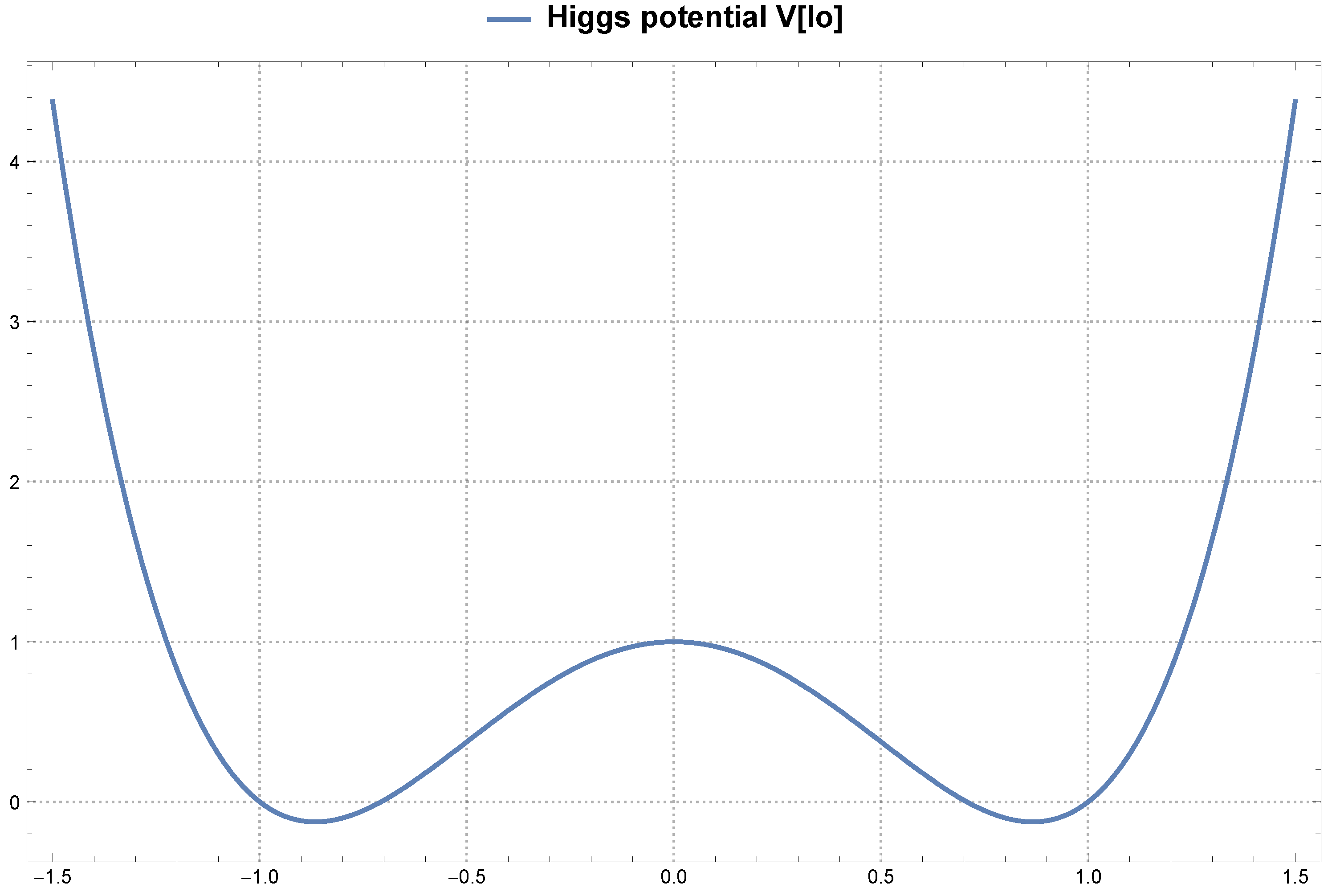
Figure 2.
Weyl tensor component as a wave.
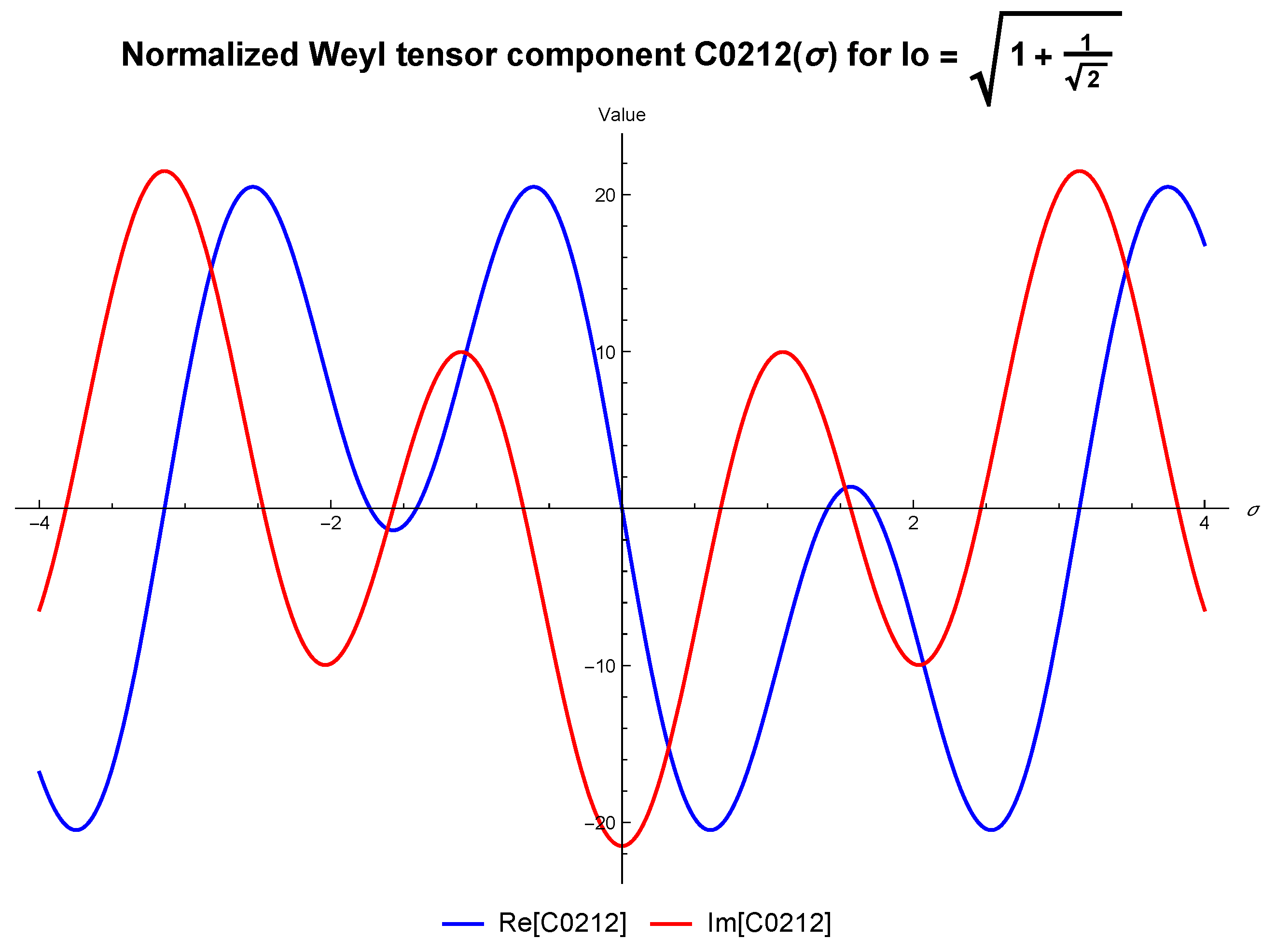
Figure 3.
Deformation visualization for particles on a circle.
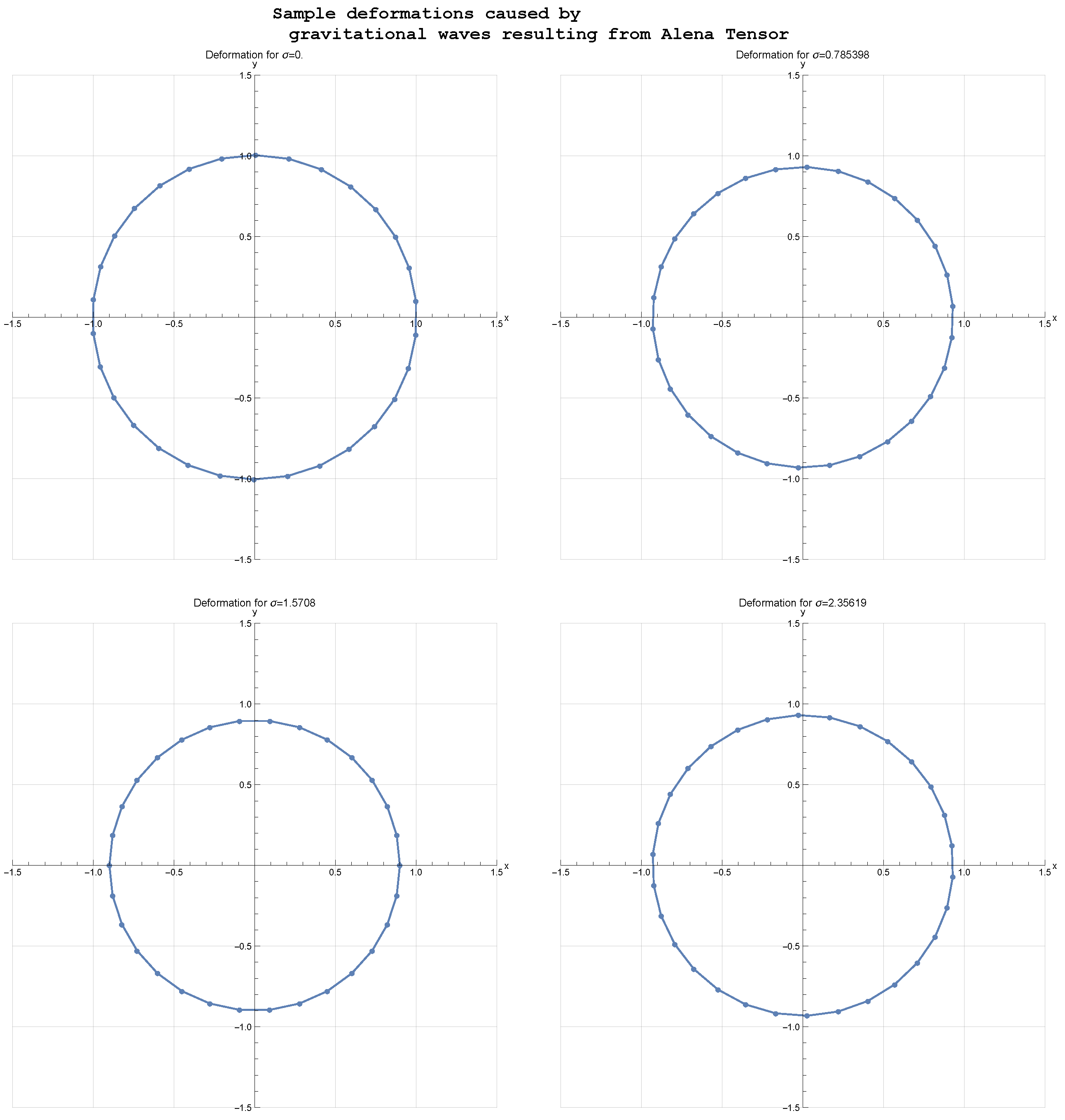
Disclaimer/Publisher’s Note: The statements, opinions and data contained in all publications are solely those of the individual author(s) and contributor(s) and not of MDPI and/or the editor(s). MDPI and/or the editor(s) disclaim responsibility for any injury to people or property resulting from any ideas, methods, instructions or products referred to in the content. |
© 2025 by the authors. Licensee MDPI, Basel, Switzerland. This article is an open access article distributed under the terms and conditions of the Creative Commons Attribution (CC BY) license (http://creativecommons.org/licenses/by/4.0/).
Copyright: This open access article is published under a Creative Commons CC BY 4.0 license, which permit the free download, distribution, and reuse, provided that the author and preprint are cited in any reuse.


