Preprint
Article

This version is not peer-reviewed.

Time-Like Extra Dimensions: Quantum Nonlocality, Spin, and Tsirelson Bound

A peer-reviewed article of this preprint also exists.

Submitted:

29 January 2025

Posted:

30 January 2025

You are already at the latest version

Abstract

The E8 ⊗ E8 octonionic theory of unification suggests that our universe is six-dimensional and that the two extra dimensions are timelike. These timelike extra dimensions, in principle, offer an explanation of the quantum nonlocality puzzle, also known as the EPR paradox. Quantum systems access all six dimensions whereas classical systems such as detectors experience only four dimensions. Therefore, correlated quantum events which are timelike separated in 6D can appear to be spacelike separated, and hence nonlocal, when projected to 4D. Our lack of awareness of the extra timelike dimensions creates the illusion of nonlocality whereas in reality the communication obeys special relativity and is local. Bell inequalities continue to be violated because quantum correlations continue to hold. In principle, this idea can be tested experimentally. We develop our analysis after first constructing the Dirac equation in 6D using quaternions, and using the equation to derive spin matrices in 6D and then in 4D. We also show that the Tsirelson bound of the CHSH inequality can in principle be violated in 6D.

Keywords: 
;  ;  ;  ;  

1. Introduction

The EPR paradox notes the following property of quantum mechanics. Given a correlated pair of say two quantum subsystems, a measurement on one subsystem influences the other subsystem non-locally. This property has been confirmed by experiments and is equivalent to the confirmation that quantum systems violate Bell’s inequalities. Such a Bell-type measurement cannot be used to transmit information faster than light; therefore the laws of special relativity are not violated, in spite of there being a nonlocal influence. One could accept this peculiarity as an inevitable feature of quantum mechanics and assert that the collapse of the wavefunction is accompanied by a nonlocal effect, and there is nothing more to be explained. Alternatively, one could insist that the following needs to be explained: what is the physical mechanism whereby subsystems in a correlated quantum system impact each other outside the light cone [1,2]? Could it be that our understanding of spacetime structure in quantum theory is incomplete? It is this latter stance which is adopted in the present brief article, and a simple solution is proposed, which removes this tension between quantum mechanics and special relativity, without altering the laws of either theory.
Our proposal is that the spacetime of our universe is not four-dimensional, but six-dimensional. And that the two extra dimensions are timelike. Laws of special relativity hold also in this bigger spacetime with signature ( 3 , 3 ) and influence of wave function collapse takes place locally in 6D spacetime. Correlated events that are time-like separated in 6D can appear to be spacelike separated in 4D, giving rise to the EPR paradox. Bell’s inequalities continue to be violated, in 6D as well as in 4D. This is so because the violation is equivalent to ruling out a deterministic locality. Indeterministic locality is permitted (which is what gives rise to higher-than-classical quantum correlations). In 4D, this translates into an apparent indeterministic nonlocality, giving rise to the illusion of a conflict between quantum mechanics and relativity.
In the next section, we briefly introduce the Dirac equation in 6D spacetime. Also, one can embed two 4D spacetime manifolds in 6D, having relatively flipped signatures. Classical systems, including detectors, live in only one of the two 4D submanifolds. In Section 3 we use the Dirac equation to derive spin matrices in 6D and then in 4D. In Section 4, we explain the resolution of the EPR paradox in some detail and comment on the hypothetical possibility of its experimental validation. In Section 5 we describe the motivation for extra time-like dimensions coming from our ongoing research program of gravi-weak unification. In Section 6 we note that the Tsirelson bound in the CHSH inequality can sometimes be violated.

2. Some Remarks on Dirac Equation in 6D Spacetime

2.1. Dirac Equation Using Gamma Matrices

We start with the 6D spacetime manifold M 6 with the coordinates ( t 1 , t 2 , t 3 , x 1 , x 2 , x 3 ) and signature (+, +, +, -, -, -). The Minkowski metric having the isometry group S O ( 3 , 3 ) is
d s 2 = d t 1 2 + d t 2 2 + d t 3 2 d x 1 2 d x 2 2 d x 3 2
The trajectory of a particle in M 6 can be identified by the functions t i ( τ ) , x i ( τ ) where τ is the proper time in M 6 . The Klein-Gordon equation is
( + m 2 ) ψ = 0 ; = t 1 2 + t 2 2 + t 3 2 x 1 2 x 2 2 x 3 2
We assume that prior to the electroweak symmetry breaking the universe is endowed with a 6D spacetime. The (chiral) symmetry breaking gives rise to two overlapping 4D spacetimes, one of which we are familiar with and whose pseudo-Riemannian geometry is determined by the laws of general relativity. The other 4D spacetime has a signature flipped with respect to ours, and its pseudo-Riemannian geometry can be shown to be a gravity-type interpretation of the weak force. The two spacetimes have one time and one space dimension in common. The two time dimensions of the other spacetime which are not part of this intersection can be interpreted as the internal symmetry directions overlaid (as a vector bundle) on our 4D spacetime. Prior to the symmetry breaking, gravitation and the electroweak interaction are unified into a 6D (non-chiral) theory of gravitation [3].
The following resolution of the EPR paradox depends only on there being a 6D spacetime of signature (3,3). It is independent of the above theoretical motivation for the 6D spacetime, coming from our approach to gravi-weak unification.
Inside the 6D spacetime, the 4D submanifold M 4 with symmetry S O ( 1 , 3 ) has the coordinates ( t 1 , x 1 , x 2 , x 3 ) with the signature (+,-,-,-). A second 4D submanifold M 4 with symmetry S O ( 3 , 1 ) can be chosen to be ( x 1 , t 1 , t 2 , t 3 ) which has the signature (-,+,+,+). Instead of choosing x 1 , we could also choose x, which is any linear combination of x 1 , x 2 and x 3 . This shows that there is a common plane ( t 1 , x ) between these manifolds. We should get the 6D Dirac equation using
= ( Γ μ μ ) ( Γ ν ν )
with { Γ μ , Γ ν } = 2 η μ ν I . In the 4D case, imposing the anti-commutation conditions on the four gamma matrices, we get a 4 × 4 matrix representation. What is the possible representation in this case of six gamma matrices with ( Γ i ) 2 = I for i = 1 , 2 , 3 and ( Γ i ) 2 = I for i = 4 , 5 , 6 ? Using the Clifford algebra representation, we get spinors of dimension 2 6 / 2 = 8 and a set of 8 × 8 gamma matrices. These gamma matrices can be constructed explicitly by choosing representations and we can also construct the corresponding Lagrangian. This gives us a Dirac equation ( i Γ μ μ Q ) ψ = 0 for M 6 where Q is a general source charge and this equation should also reduce to the Dirac equation in M 4 as we will see later. The 8D spinors in M 6 as we will explain, will break into two Dirac spinors, one belonging to the section M 4 and the other belonging to the section M 4 . Thus, we will be able to write
ψ M 6 = ψ M 4 + ψ M 4
This will allow us to understand that the quantum state is a superposition across these two submanifolds. We also need to define a new Hilbert space H H . We need to include more observables in our quantum system, a set of observables { A } in H, and a mirror set of observables { A } in H and some additional observables forming a complete set of observables for H H
{ A } { A } ψ M 4 ψ M 4
This describes the actions of different observables on the system in M 6 which is a superposition across M 4 and M 4 . These non-vanishing off-block-diagonal observables are the additional ones that we have to add to get a complete set. In section 3, we explicitly show how to construct the spin operators in H and H .

2.2. Dirac Operator Using Quaternions

We propose an alternative construction of the Dirac operator using quaternions. To construct the 6D Dirac operator we start with the Clifford algebra C l ( 0 , 3 ) of split biquaternions, expressed as H + ω H with ω satisfying ω ˜ = ω , ω 2 = 1 . We have pure imaginary quaternions associated with each set of quaternions as ( i ^ , j ^ , k ^ ) and ( l ^ , m ^ , n ^ ). The elements inside each set anticommute with each other, and elements of one set commute with the elements of the other set. These can be used as vectors in 3D spaces, and we would like to use them to describe our 6D spacetime. We express the events in 6D as
x 6 = t 1 i ^ + t 2 j ^ + t 3 k ^ + ω ( x 1 l ^ + x 2 m ^ + x 3 n ^ )
which gives
x 6 x 6 ˜ = t 1 2 + t 2 2 + t 3 2 x 1 2 x 2 2 x 3 2
This is the correct signature for the interval and is associated with SO(3,3). Note that this x 6 is not Hermitian. Let us denote t 1 , t 2 , t 3 , x 1 , x 2 , x 3 by the indices 01, 02, 03, 1, 2, 3. Now we construct the Dirac operator as
D 6 = i ^ 01 + j ^ 02 + k ^ 03 + ω ( l ^ 1 + m ^ 2 + n ^ 3 )
which gives us the correct Klein-Gordon operator
D 6 D 6 ˜ = 01 2 + 02 2 + 03 2 1 2 2 2 3 2
We then ask for a Dirac equation with a general source charge
i h D 6 ψ = Q ψ
This is similar to the one obtained above, but now we have quaternions instead of gamma matrices. For relating this to 4D spacetimes, this 6D Dirac operator can be broken down into two Dirac operators D 4 and D 4 .
D 4 = i ^ 01 + ω ( l ^ 1 + m ^ 2 + n ^ 3 )
which gives
D 4 D 4 ˜ = 01 2 1 2 2 2 3 2
Similarly for the Dirac operator D 4 we can write
D 4 = ω l ^ 1 + i ^ 01 + j ^ 02 + k ^ 03
This also gives the correct signature. Both these Dirac operators give the Dirac equation for M 4 and M 4 . We also note that Wilson [4] showed using S O ( 3 , 3 ) S L ( 4 , R ) and the generators of S L ( 4 , R ) having two copies of 4D spacetimes described in terms of gamma matrices and quaternions, it is easy to make maps between the quaternion vectors i ^ , j ^ , k ^ , l ^ , m ^ , n ^ and the quaternion bivectors to gamma matrices. We use this to reduce this quaternionic Dirac operator to the usual one. Use i ^ γ 0 , ω l ^ γ 1 , ω m ^ γ 2 , ω n ^ γ 3 to get the usual Dirac equation.
Alternatively, we can also construct the 4D Dirac operator as
D 4 = 0 i ( i ^ 1 + j ^ 2 + k ^ 3 )
This satisfies the above equation, and it is Hermitian. The Hermiticity is not preserved in the other cases mentioned above.

2.3. Dirac Equation Using Quaternion Bivectors

Another attempt motivated by Lambek’s work [8] was to define x 6 using the bivectors. We have 9 bivectors i ^ l ^ , j ^ l ^ , k ^ l ^ , i ^ m ^ , j ^ m ^ , k ^ m ^ , i ^ n ^ , j ^ n ^ , k ^ n ^ . In this case, the constructed x 6 will only use 6 of these bivectors and the Dirac operator will be written as
D 6 = l ^ i ^ 01 + l ^ j ^ 02 + l ^ k ^ 03 + ω ( m ^ i ^ 1 + m ^ j ^ 2 + m ^ k ^ 3 )
which gives
D 6 D 6 ˜ = 01 2 + 02 2 + 03 2 1 2 2 2 3 2 2 ω l ^ m ^ i ^ j ^ 01 2 2 ω l ^ m ^ i ^ k ^ 01 3 2 ω l ^ m ^ j ^ i ^ 02 1 2 ω l ^ m ^ j ^ k ^ 02 3 2 ω l ^ m ^ k ^ i ^ 03 1 2 ω l ^ m ^ k ^ j ^ 03 2 .
This is not giving the correct signature and one has these extra terms. They cancel when we impose the constraints
01 2 = 02 1 , 01 3 = 03 1 , 02 3 = 03 2
How do we interpret these odd relations? Based on Wilson’s work [4] this can also be related to gamma matrices as ( l ^ i ^ , l ^ j ^ , l ^ k ^ ) corresponds to ( γ 0 γ 1 , γ 0 γ 2 , γ 0 γ 3 ) and ( m ^ i ^ , m ^ j ^ , m ^ k ^ ) correspond to ( i γ 1 , i γ 2 , i γ 3 ). This means that
D 6 = γ 0 ( γ 1 01 + γ 2 02 + γ 3 03 ) + ω ( γ 1 1 + γ 2 2 + γ 3 3 )
Since γ 0 γ 1 commutes with γ 1 but not with γ 2 , we get similar extra terms while computing D 6 D 6 ˜ . This is fixed by mapping ω γ i to some new gamma matrices that complete the set of 6 gamma matrices( Γ i , Γ ˜ i ) for 6D. Let us also try to construct D 4 and D 4 from this
D 4 = l ^ i ^ 01 + ω ( m ^ i ^ 1 + m ^ j ^ 2 + m ^ k ^ 3 )
This shows that
D 4 D 4 ˜ = 01 2 1 2 2 2 3 2 2 ω l ^ m ^ i ^ j ^ 01 2 2 ω l ^ m ^ i ^ k ^ 01 3
thus again giving extra terms. We will therefore adhere to our earlier method of deriving the 6D and 4D Dirac equations from quaternions. An analogous decomposition (from 6D to 4D) of the Klein-Gordon equation can be expected to hold for bosons.

3. Interpreting Spin in 6D

In this section, we will explore the interpretation of spin by considering the non-relativistic limit of Dirac equation in 6D. By examining this limit and projecting to both M 4 and M 4 , we aim to identify the spin matrices. This framework can potentially faciliate in understanding the behavior of spin in the presence of additional time-like dimensions. Therefore, consider the Dirac equation of the form,
i Γ μ μ Q Φ = 0
where the set of gamma matrices are
[ Γ ^ 3 , 3 ] = Γ ˜ 3 , Γ ˜ 2 , Γ ˜ 1 , Γ 1 , Γ 2 , Γ 3
such that
{ Γ μ , Γ ν } = 2 η μ ν 1 8
where, η μ ν = diag ( + 1 , + 1 , + 1 , 1 , 1 , 1 ) . Here, Γ ˜ i 2 = 1 8 , and Γ i 2 = i 8 2 for i = 1 , 2 , 3 . Let us introduce the following decomposition,
Γ ˜ i = i B λ i ( i = 1 , 2 , 3 )
Γ i = B α i ( i = 1 , 2 , 3 )
such that
{ α i , α j } = 0 ( i j )
{ λ i , λ j } = 0 ( i j )
{ α i , λ j } = 0 ( i , j )
α i 2 = λ i 2 = B 2 = 1
Then, the Dirac equation can be written in a suitable form
i λ i ˜ i Φ = i α i i + B Q Φ
To take the non-relativistic limit, we will choose a basis wherein,
α i = Σ i 0 1 1 0
λ i = Σ ˜ i 1 0 0 1
B = 1 0 0 1
Σ ˜ i , Σ j ] = 0 ( i , j )
and decompose Φ as,
Φ = ϕ 1 ϕ 2 = φ 1 φ 2 φ 3 φ 4
where, both ϕ 1 and ϕ 2 are Dirac spinors. Substituting (35) into (30), we get,
i Σ ˜ i ˜ i 0 0 Σ ˜ i ˜ i ϕ 1 ϕ 2 = i 0 Σ i i Σ i i 0 + 1 0 0 1 Q ϕ 1 ϕ 2
The source charge matrix Q in our choice of bases is,
Q = m 0 0 0 0 0 0 m 0 0 m 0 0 m 0 0
This results in a system of four coupled differential equations
i ( Σ ˜ i ˜ i ) φ 1 = i ( Σ i i ) φ 3 + m φ 1
i ( Σ ˜ i ˜ i ) φ 2 = i ( Σ i i ) φ 4 + m φ 4
i ( Σ ˜ i ˜ i ) φ 3 = i ( Σ i i ) φ 1 m φ 3
i ( Σ ˜ i ˜ i ) φ 4 = i ( Σ i i ) φ 2 m φ 2
where, [ Σ ˜ i , Σ ˜ j ] = i ϵ i j k Σ ˜ k and [ Σ i , Σ j ] = i ϵ i j k Σ k .

3.1. Non-Relativistic Limit (v/c) Expansion for the First Dirac Spinor ( M 4 )

Consider the Dirac equation,
i λ i ˜ i Φ = i α i i + e A 0 + B Q Φ
Let us now consider,
i ( Σ ˜ i ˜ i ) φ 1 = i ( Σ i i ) φ 3 + e A 0 φ 1 + m φ 1
i ( Σ ˜ i ˜ i ) φ 3 = i ( Σ i i ) φ 1 + e A 0 φ 3 m φ 3
and decompose φ 1 and φ 3 as follows to describe them as slowly varying functions:
φ 1 e i m t i φ 1
φ 3 e i m t i φ 3
Substituting these into (38) and (40) gives us,
Σ ˜ i ( m + i ˜ i ) φ 1 = i ( Σ i i ) φ 3 + e A 0 φ 1 + m φ 1
Σ ˜ i ( m + i ˜ i ) φ 3 = i ( Σ i i ) φ 1 + e A 0 φ 3 m φ 3
In the non-relativistic limit, m e A 0 , we have,
e A 0 0
Σ ˜ i ˜ i 0
So, (48) becomes,
( Σ ˜ i m + m ) φ 3 = i ( Σ i i ) φ 1
Substituting (51) into (47), we get,
Σ ˜ i ( m + i ˜ i ) φ 1 = ( Σ i i ) 2 ( Σ ˜ i m + m ) 1 φ 1 + e A 0 φ 1 + m φ 1
Projecting to the spacetime M 4 with signature η μ ν = diag ( + 1 , 1 , 1 , 1 ) , we impose the following,
Σ ˜ i 1
i ˜ i i t
Hence, (52) becomes
1 ( m + i t ) φ 1 = ( Σ i i ) 2 ( 1 m + m ) 1 φ 1 + e A 0 φ 1 + m φ 1
i t = 1 2 m ( Σ i i ) 2 + e A 0
We have recovered Pauli’s equation which is typically represented as,
i t = 1 2 m ( σ · p ^ ) 2 + q ϕ
Comparing (55) and (57), we see that Σ i are the spatial spin matrices.

3.2. Non-Relativistic Limit (v/c) Expansion for the Other Dirac Spinor ( M 4 )

The source charge term m should be e 2 and the coupling factor is m instead of e (we explain the reason for this in Section 5). Following along with the previous section, let us now consider,
i ( Σ ˜ i ˜ i ) φ 2 = i ( Σ i i ) φ 4 + m A ˜ 0 φ 4 + e 2 φ 4
i ( Σ ˜ i ˜ i ) φ 4 = i ( Σ i i ) φ 2 + m A ˜ 0 φ 2 e 2 φ 2
Decompose φ 2 and φ 4 as follows:
φ 2 e i e 2 x i φ 2
φ 4 e i e 2 x i φ 4
Substituting these into (58) and (59) gives us,
i ( Σ ˜ i ˜ i ) φ 2 = Σ i ( e 2 + i i ) φ 4 + m A ˜ 0 φ 4 + e 2 φ 4
i ( Σ ˜ i ˜ i ) φ 4 = Σ i ( e 2 + i i ) φ 2 + m A ˜ 0 φ 2 e 2 φ 2
Taking the non-relativistic limit, e 2 m A ˜ 0 ,
m A ˜ 0 0
Σ i i 0
Hence, (63) becomes,
i ( Σ ˜ i ˜ i ) φ 4 = ( Σ i e 2 + e 2 ) φ 2
Substituting (66) in (62) we get,
Σ i ( e 2 + i i ) φ 4 = ( Σ ˜ i ˜ i ) 2 ( Σ i e 2 + e 2 ) 1 φ 4 + m A ˜ 0 φ 4 + e 2 φ 4
Projecting to the spacetime M 4 with signature η μ ν = diag ( 1 , 1 , 1 , + 1 ) , we impose the following,
Σ i 1
i i i x
Hence, (67) becomes
1 ( e 2 + i x ) φ 4 = ( Σ ˜ i ˜ i ) 2 ( 1 e 2 + e 2 ) 1 φ 4 + m A ˜ 0 φ 4 + e 2 φ 4
i x = 1 2 e 2 ( Σ ˜ i ˜ i ) 2 + m A ˜ 0
Owing to the resemblance with Pauli’s Equation (57), we identify Σ ˜ i to be the temporal spin matrices. Now, the spatial spin matrices are associated with M 4 and the temporal spin matrices are associated with M 4 , which gives an interpretation of spin in 6D.

4. Proposed Resolution of the EPR Paradox

4.1. Proposal

Suppose Alice and Bob are spacelike separated inertial observers in our 4D spacetime who are stationary with respect to each other. Both of them have one electron/positron each from a pair in an entangled state. When Alice makes an observation on her electron, the wave function of Bob’s positron seems to collapse as if it violates locality. Local hidden variable theories were introduced to understand this but Bell inequalities show that such theories have an upper bound, and quantum theories violate that bound showing that local hidden variable theories cannot explain experiments. Quantum theory goes against local realism, and any hidden variable theory must be non-local.
We propose that the non-locality puzzle can be resolved in the presence of a 6D spacetime of signature ( 3 , 3 ) 
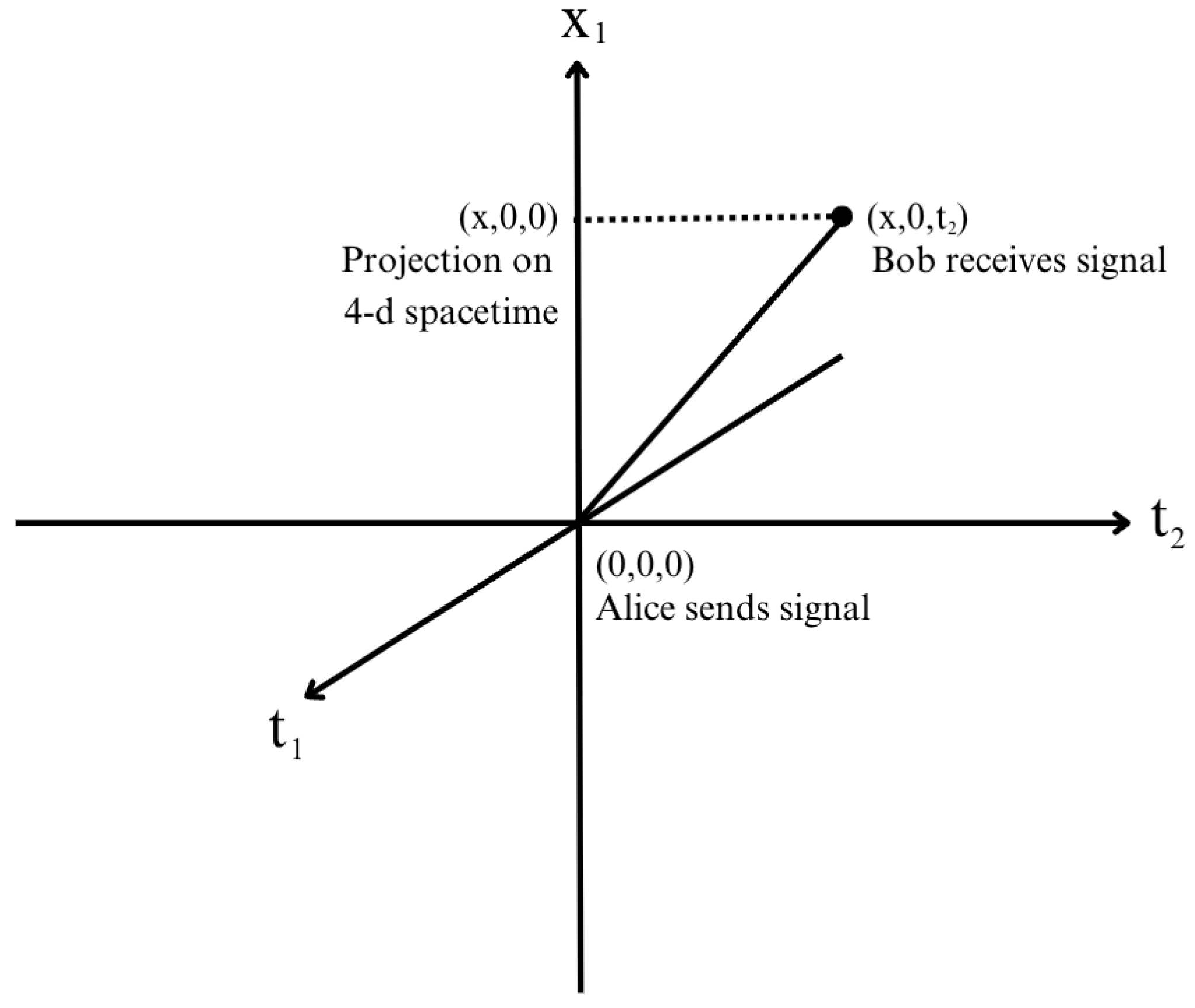
, and by assuming that the electron-positron pair traverse the 6D spacetime, not 4D spacetime. Consider the 3D illustration of Figure 1 where x 1 , t 1 are dimensions in our 4D spacetime and t 2 is a timelike dimension in 6D.
From Figure 1, the Minkowski space-time interval can be mathematically expressed as the following line element:
d s 2 = d t 2 2 + d t 1 2 d x 1 2
Choose d t 2 , d t 1 , and d x 1 such that the path defined by this line element is inside the light cone of this 3D spacetime ( t 2 , t 1 , x 1 ) which has signature ( + , + , ) , namely two time-like and one space-like directions. In other words, d s 2 > 0 . Now consider the case that even when d t 1 = 0 , the line element is time-like. That is,
d s 2 = d t 2 2 d x 1 2
is positive.
Consider the 2D spacetime ( t 1 , x 1 ) [which represents our spacetime in which Alice and Bob make measurements]. In such a case, while observing the event, we will naturally assume d t 2 = 0 and conclude that d s 2 = d x 1 2 < 0 and that the separation between the sending of a signal and the receiving of the signal is spacelike and hence nonlocal. This is as though faster-than-light influence has taken place. However, in the 3D universe, the event is local and obeys special relativity.
Thus, the EPR paradox can be resolved if there is an additional time-like direction in the universe. Classical systems do not probe the t 2 direction. Only quantum systems, which obey quantum linear superposition, probe t 2 . A photon travelling from Alice to Bob travels along a path which is a quantum superposition of a path in ( t 1 , x 1 ) and a path in ( t 2 , x 1 ) . If we do not know of the photon path in the other submanifold, that lack of knowledge gives rise to the EPR paradox.
In essence, we are saying that the path through the other sub-manifold is shorter than the path in ours and takes less time to traverse. The spatial coordinate separation is just d x 1 , which is the same in both submanifolds. But the proper physical spatial distance depends on the spacetime metric, and this metric can be different in the two sub-manifolds, making the path in the other sub-manifold shorter in spatial distance, and hence it is covered in less time. If L 2 is the proper spatial distance in the other submanifold and L 1 is the proper spatial distance in the usual 4D spacetime, then L 2 L 1 . Light takes time d t 2 = L 2 / c to travel from Alice to Bob in the other submanifold. In our 4D spacetime, the amount of t 1 time elapsed while a distance L 2 is covered in the other universe is L 2 / c , which is far less than the actual travel time L 1 / c in our 4D spacetime. The arrival at Bob appears instantaneous to us; which is why we set d t 1 = 0 .

4.2. Experimental Validation

Consider that Alice makes a measurement that causes the electron state to collapse. The signal carrying information about the collapse travels from Alice to Bob (through M 4 ) at the speed of light, arriving at the correlated positron after a time t 1 P = L 2 / c . Clearly, the influence on the positron is not instantaneous but takes a finite time t 1 P (howsoever small). If Bob makes his measurement on the positron prior to time t 1 P , i.e., prior to the arrival of information of collapse from Alice, evidently the correlation will not have been established. The results of Bob’s measurements in this case will not show a violation of Bell’s inequalities. The inequalities will only be violated if Bob’s measurements are made later than time t 1 P . In principle, this feature can be tested experimentally.
In practice, however, the experiment is extremely challenging, and essentially impossible, with current technology. This is because, in our research program of gravi-weak unification, the pseudo-Riemannian geometry of the manifold M 4 is determined by the weak force. Whereas in our spacetime M 4 , the cosmic horizon is at about 10 28 cm, in M 4 this same horizon is at the range of the weak force, namely about 10 16 cm. In other words, lengths are scaled down by an enormous factor 10 44 , and through M 4 light will travel from our location to the cosmic horizon in merely 10 26 s, which of course for all practical purposes is instantaneous. Therefore, in reality, t 1 P < 10 26 s and a Bell test of the 6D spacetime idea is simply impossible. An observer unaware of the 6D spacetime will infer that the signal travelled through our 4D spacetime at a staggering speed of 10 44 c. This is far, far greater than the lower experimental bound of about 10 5 c on the speed of such a correlation signal (assuming that collapse information travels through our 4D spacetime at the speed of light) [5]. This experimental bound also tells us that the shrinking of lengths in M 4 , relative to M 4 , is at least by a factor of 10 5 .
An important caveat in the above reasoning was brought to our attention by Gisin [6]. When the measurements by Alice and Bob are spacelike separated, there is no definite causal order (past to future) between Alice’s measurement and Bob’s measurement - the ordering is frame-dependent. Therefore, such an experiment as the one proposed above, if at all it could be done, will have to be in a universal absolute time, say in the rest frame of the cosmic microwave background.
The second path through M 4 could be suggestively called a `quantum wormhole’. Our proposal can also be viewed as a rigorous realisation of the ER=EPR idea [7]. Instead of the Einstein-Rosen bridge, we have an extremely short space-time path connecting Alice and Bob through the second spacetime. It will be interesting to study black-hole solutions in 6D spacetime, and enquire how such black holes relate to black hole solutions in M 4 and in M 4 .

5. Physical Motivation for Two Timelike Extra Dimensions

There is considerable literature on physics in six-dimensional spacetimes with signature ( 3 , 3 ) . The motivations for such considerations are varied, starting with desiring as many time dimensions as spatial ones. Quaternions also point to a 6D spacetime, as Lambek explains in his paper titled `Quaternions and three temporal dimensions’ [8]. He writes in the abstract of his paper: “The application of quaternions to special relativity predicts a six-dimensional universe, which uncannily resembles ours, except that it admits three dimensions of time. Yet its mathematical description with the help of quaternions gains in transparency, due to the crucial observation that every skew-symmetric four-by-four real matrix is the sum of two matrices representing multiplication by vector quaternions on the left and the right respectively.”
In an insightful paper titled `Germ of a synthesis: space-time is spinorial, extra dimensions are time-like’ Sparling [9] observes the relation of null twistor spaces with 6D spacetime. It is worthwhile to quote from his abstract:
First, an integral transform is introduced into Einstein’s general relativity that is non-local and spinorial. For Minkowskian space-time, the transform intertwines three spaces of six dimensions, which a priori are on an equal footing, linked by the octavic triality of Cartan. Two of these spaces are interpreted as null twistor spaces; the third may be regarded as giving space-time two extra time-like dimensions, for which the ordinary space-time is an axis of symmetry.
Second, it is suggested that the extra dimensions perdure for a general space–time: the overall structure is controlled by a generalized Fefferman tensor. Accordingly, it is posited that the additional time-like dimensions arise naturally and constitute an aspect of space-time reality that ultimately will be amenable to experimental investigation.
Highly relevant for us is also the (1985) paper of Patty and Smalley [10] titled `Dirac equation in a six-dimensional spacetime’. The authors show that a (3+3) spacetime can be divided into six copies of (3+1) subspaces. 6D spaces are also of interest from the viewpoint of a superluminal extension of (3+1) special relativity, and it has been shown that a 6D spacetime is the smallest one which can accommodate a superluminal as well as a subliminal branch of (3+1) spacetime [11]. Six dimensional = (3+3) spacetimes were studied extensively in a series of papers by Cole [12] and also by Teli [13]. An early work on `quaternions and quantum mechanics’ is Conway (1948) [14]. Very relevant for us is also Kritov (2021) [15] who shows that the Clifford algebra C l ( 3 , 0 ) can be used to make two copies of 4D spacetime with relatively flipped signatures. Dartora and Cabrera (2009) [16] have studied `The Dirac equation in six-dimensional SO(3,3) symmetry group and a non-chiral `electroweak theory’. An old (1950) paper by Podolanski [17] studies unified field theory in six dimensions, and in fact the abstract starts by saying `The geometry of the Dirac equation is actually six-dimensional’. An elegant (2020) paper by Venancio and Batista [18] analyses `Two-Component spinorial formalism using quaternions for six-dimensional spacetimes’. An insightful (1993) work by Boyling and Cole [19] studies the six-dimensional (3+3) Dirac equation and shows that particles have spatial spin-1/2 and temporal spin-1/2. See also Brody and Graefe (2011) [20]. Shtanov and Sahni studied a five-dimensional cosmological model with two time-like dimensions [21]. Interestingly, such a universe bounces at high densities and the nature of the bounce is similar to that in loop quantum cosmology.
Our interest in 6D spacetime stems from the ongoing research program on unification, known as the E 8 E 8 octonionic theory of unification, and recently reviewed in Singh (2024) [3]. This pre-spacetime, pre-quantum theory is a matrix-valued Lagrangian dynamics on a split bi-octonionic space, which obeys the E 8 E 8 unified symmetry prior to the electroweak symmetry breaking. This is also the gravi-weak symmetry breaking, wherein each of the two E 8 -s branch into four S U ( 3 ) s. The net result is a 6D spacetime of signature ( 3 , 3 ) broken into two overlapping 4D spacetimes M 4 and M 4 and six emergent forces. Four of these are currently known to us, and two new forces are predicted, these being S U ( 3 ) g r a v and U ( 1 ) D E M . On M 4 , the breaking S U ( 3 ) S U ( 2 ) L U ( 1 ) Y U ( 1 ) e m gives rise to the weak force as pseudo-Riemannian geometry of M 4 , with the unbroken sector S U ( 3 ) c o l o r U ( 1 ) e m providing the geometry of the vector bundle. The quantum number associated with U ( 1 ) e m is the electric charge e. Correspondingly, on M 4 , the breaking of another S U ( 3 ) S U ( 2 ) R U ( 1 ) Y D E M U ( 1 ) D E M gives rise to general relativity as the pseudo-Riemannian geometry of M 4 , with the unbroken sector S U ( 3 ) g r a v U ( 1 ) D E M providing the geometry of the vector bundle. DEM stands for dark electromagnetism and the quantum number associated with U ( 1 ) D E M is the square root of mass m (this is the reason for the interchange e m in Section 3 when going from M 4 to M 4 ).
Thus, the weak force is the space-time geometry of M 4 and general relativity is the space-time geometry of M 4 . Both interactions are chiral, the former being left-handed, and the latter right-handed. Together, they are unified into a (non-chiral) gravi-weak symmetry on 6D spacetime, prior to the electroweak symmetry breaking. A detailed analysis leading to these results will be presented in a forthcoming paper [22]. Thus, in our unification program, it is natural to consider a 6D spacetime with signature (3,3) as physical reality.

6. Tsirelson Bound

Bell’s theorems are a set of closely related results which imply that quantum mechanics is incompatible with local hidden variable theories. Bell’s inequality is the statement that when measurements are performed independently on two space-like separated particles in an entangled pair, the assumption that outcomes depend on local hidden variables implies an upper bound on the correlations between the outcomes. As we know, quantum mechanics predicts correlations which violate this upper bound. The CHSH inequality is a particular Bell inequality in which classical correlation (i.e., if local hidden variables exist) can take the maximum value of 2. Quantum mechanics violates this bound, allowing for a higher bound on the correlation, which can take the maximum value 2 2 , known as the Tsirelson bound [23]. Popescu and Rohrlich [24] showed that the assumption of relativistic causality allows for an even higher bound on the CHSH correlation, this value being 4. It is important to ask why the bound coming from causality is higher than the Tsirelson bound. Are there relativistic causal dynamical theories which violate the Tsirelson bound? In a recent paper [25], we found this to indeed be the case. We showed that the pre-quantum theory of trace dynamics, from which quantum theory is emergent as a thermodynamic approximation, permits the CHSH correlation to take values higher than 2 2 . We interpreted our findings to suggest that quantum theory is approximate and emergent from the more general theory of trace dynamics.
What impact does the extension of spacetime to 6D have on the Tsirelson bound on quantum correlations? Our analysis below suggests that in this scenario as well, the Tsirelson bound could be beaten.
Suppose the system under analysis is entangled, described by ψ 1 , the state prepared by us. The situation is the same as what is discussed in the EPR paradox. Consider the superposition state ψ = α ψ 1 + β ψ 2 (over the two spacetimes M 4 and M 4 ) and let us find out what happens to the correlations E ( A B ) . The expectation value of the correlation E ( A B ) is given by:
E ( A B ) = ψ | A B | ψ
Substituting ψ = α ψ 1 + β ψ 2 , we get
E ( A B ) = ( α ψ 1 + β ψ 2 ) | A B | ( α ψ 1 + β ψ 2 )
Using the linearity of the inner product and factoring out constants:
E ( A B ) = | α | 2 ψ 1 | A B | ψ 1 + α * β ψ 1 | A B | ψ 2 + β * α ψ 2 | A B | ψ 1 + | β | 2 ψ 2 | A B | ψ 2
There is an important contribution from cross-terms that may not be zero even if the states are orthogonal. This occurs because the operator AB defined on the complete Hilbert space can rotate ψ 2 in such a way that it positions it at an angle other than 90 deg relative to ψ 1 . This happens because of the off-block-diagonal terms in (5). Note that the states are normalised, that is, | α | 2 + | β | 2 = 1 . What we can now do is identify the real number coming from the cross-terms as
r A B = α * β ψ 1 | A B | ψ 2 + β * α ψ 2 | A B | ψ 1
The CHSH correlation function F is given by:
F = E ( A , B ) + E ( A , B ) + E ( A , B ) E ( A , B )
This can be expressed as:
F = | α | 2 F 1 + | β | 2 F 2 + r ; r = r A B + r A B + r A B r A B
where F 1 and F 2 are defined as :
F 1 = ψ 1 | A B | ψ 1 + ψ 1 | A B | ψ 1 + ψ 1 | A B | ψ 1 ψ 1 | A B | ψ 1
F 2 = ψ 2 | A B | ψ 2 + ψ 2 | A B | ψ 2 + ψ 2 | A B | ψ 2 ψ 2 | A B | ψ 2
We compute the squares of F 1 and F 2
F 1 2 = ψ 1 | 4 I [ A , A ] [ B . B ] | ψ 1
F 2 2 = ψ 2 | 4 I [ A , A ] [ B . B ] | ψ 2
The square of F, i.e., F 2 , in terms of F 1 , F 2 and r is given by:
F 2 = | α | 4 F 1 2 + 2 | α | 2 | β | 2 F 1 F 2 + | β | 4 F 2 2 + r 2 + 2 r ( | α | 2 F 1 + | β | 2 F 2 )
Now for the case of the normalized state a 2 + b 2 = 1 , where a = | α | and b = | β | . Using the upper bounds F 1 2 8 and F 2 2 8 and the AM-GM (arithmetic mean - geometric mean) inequality, the expression simplifies to:
F 2 8 ( a 4 + b 4 ) + a 2 b 2 ( F 1 2 + F 2 2 ) + r 2 + 2 r ( | α | 2 F 1 + | β | 2 F 2 )
which then gives us
F 2 8 ( a 4 + b 4 ) + 16 a 2 b 2 + r 2 + 2 r ( | α | 2 F 1 + | β | 2 F 2 ) 8 + r 2 + 4 2 r
This shows the possibility that the Tsirelson bound can be violated in some cases, provided r > 0 , or r < 4 2 . If 4 2 r 0 the CHSH inequality is obeyed. For r = 4 2 2 , the Popescu-Rohrlich bound of 4 on the CHSH correlation F is reached. Curiously, this numerical value 4 2 2 is precisely the gap between the PR value 4 and the Tsirelson bound of 2 2 . By defining the variable z = r + 2 2 the contribution of the cross-terms can be suggestively written as ( z 2 ( 2 2 ) 2 ) , showing z to be the measure of violation of the Tsirelson bound. The bound is obeyed when | z | 2 2 and violated if | z | > 2 2 . The PR bound is equivalent to | z | = 4 . Considering how r was defined in Eqn. (79) above, it seems to be the case that these cross-terms are precisely the missing link between the Tsirelson bound and the Popescu-Rohrlich bound.
It could be that current experiments are unable to detect supra-quantum nonlocal correlations precisely because the consequences of the cross-terms (which make r non-zero) are very hard to detect. This is for the same reasons as mentioned in Section 5; i.e., the transmission through the path in M 4 is enormously quick.
Also, the challenge for appropriate experiments is that whichever observables we currently measure act only on ψ 1 , they never rotate ψ 1 outside of M 4 ; at least, we cannot claim this theoretically. For the observables that do such rotations, one might wonder if they correspond to any physical quantity. Our assessment is that such observables will be physical; they likely relate to the weak interaction, since the weak interaction determines the spacetime geometry of M 4 . Therefore, it could be that high energy experiments proposed to test Bell’s inequalities at colliders [26] might be the ideal place to look for violation of the Tsirelson bound. Because such experiments are likely to be sensitive to the weak scale.
Considering that the weak force is the spacetime geometry of M 4 , there ought to exist weak waves, analogous to gravitational waves and electromagnetic waves, but having wavelengths smaller than 10 16 cm. If ever such waves are detected in experiments, they could be a possible indicator of 6D spacetime.
The presence of three times sometimes raises enquiry as to their physical implications. For instance, which of these is the time that flows, and hence defines an arrow of time? Our stance is that these three times are time coordinates, on the same footing as the three spatial coordinates. They are mechanistic and reversible, and cannot by themselves provide a time arrow. The role of fundamental time is played by a parameter which by itself is not part of the space-time manifold. In our research program, such a parameter is the so-called Connes time in non-commutative geometry, whose origin lies in the Tomita-Takesaki theorem for von Neumann algebras [27].

7. Conclusion

We demonstrated a possible resolution of the EPR paradox by adding extra timelike coordinates. This required the quantum system to be in superposition across M 4 and M 4 and this was shown for spinors using the Dirac equation in 6D. We constructed the 6D Dirac equation using the split biquaternions and analysed how this reduces to the Dirac equation in M 4 and M 4 . It was also crucial for the argument to interpret spin in both these submanifolds. This was achieved by associating Pauli spin matrices to both these submanifolds using the non-relativistic limit of the Dirac equation to get Pauli equations for M 4 and M 4 . An experimental validation was also proposed and it was shown that the Tsirelson bound can be violated in some cases because of the presence of interference terms arising when the 6D spacetime is decomposed into two 4D spacetimes and additional operators on the Hilbert space which rotate ψ M 4 such that it leaves a component in ψ M 4 .

Acknowledgments

For participation in the early stages of this work, we would like to thank Arpit Chhabra, Yash Gupta, Satwik Mittal, Abhijeet Mohanty, and Aaayush Srivastav. For helpful discussions, it is a pleasure to thank Priyanka Giri, Nicolas Gisin, Jose Isidro, Nehal Mittal, Hendrik Ulbricht, and Harald Weinfurter.

References

  1. N. Gisin. Quantum nonlocality: How does nature do it? Science 2009, 326, 1357. [Google Scholar] [CrossRef] [PubMed]
  2. T. Maudlin. Quantum non-locality and relativity - metaphysical intimations of modern physics, 3rd Edn. ed; Wiley-Blackwell, 2011. [Google Scholar]
  3. T. P. Singh. Trace dynamics, octonions, and unification: An E8E8 theory of unification. J. Phys. Conf. Series 2024, 2912, 012009. [Google Scholar] [CrossRef]
  4. R. A. Wilson. Remarks on the group-theoretical foundations of particle physics. 2020. Available online: https://www.newton.ac.uk/files/preprints/ni19011.pdf.
  5. Daniel Salart, Augustin Baas, Cyril Branciard, Nicolas Gisin and Hugo Zbinden. Testing the speed of spooky action at a distance. Nature 2008, 454, 861–864. [Google Scholar] [CrossRef] [PubMed]
  6. N. Gisin. Session 5: Open Discussion. Time Stamp 25:00, Conference on 100 years of quantum mechanics, IISER Kolkata. 2024. Available online: https://www.youtube.com/live/KcWmBW6PyfE?si=jOVqsRI2xOGRM4mR.
  7. Maldacena, Juan and Susskind, Leonard. Cool horizons for entangled black holes. Fortschritte der Physik 2013, arXiv:1306.053361, 781–811. [Google Scholar] [CrossRef]
  8. J. Lambek. Quaternions and three temporal dimensions. 2014. Available online: https://www.math.mcgill.ca/barr/lambek/pdffiles/Quater2014.pdf.
  9. G. A. Sparling. Germ of a synthesis: Space-time is spinorial, extra dimensions are time-like. Proc. R. Soc. A. 2007, 463, 463. [Google Scholar]
  10. C. E. Patty, Jr. and L. L. Smalley. Dirac equation in a six-dimensional spacetime: temporal polarisation for subluminal interactions. Phys. Rev. D 1985, 32, 891. [Google Scholar] [CrossRef] [PubMed]
  11. W. E. Hagston and I. D. Cox. An extended theory of relativity in a six-dimensional manifold. Foundations of Physics 1985, 15, 773. [Google Scholar] [CrossRef]
  12. E. A. B. Cole and S. A. Buchanan, Space-time transformations in six-dimensional special relativity, J. Phys. A: Math. Gen. 15, L255 (1982).
  13. M. T. Teli, General Lorentz transformations in six-dimensional spacetime, Phys. Lett. A 122, 447 (1987) and references therein.
  14. A.W. Conway, Quaternions and quantum mechanics, Pontificia Academia Scientiarum, 12, 204 (1948), Available athttps://www.pas.va/content/dam/casinapioiv/pas/pdf-volumi/acta/acta12pas.
  15. A. Kritov, Gravitation with cosmological term, expansion of the universe as uniform acceleration in Clifford coordinates, Symmetry, 2021, 13 (2021).
  16. C. A. Dartora and G. G. Cabrera, The Dirac Equation in Six-dimensional SO(3,3) Symmetry Group and a Non-chiral “Electroweak” Theory, Int. J. Theo. Phys. 49, 51 (2010).
  17. J. Podolanski, Unified field theory in six dimensions, Proceedings of the Royal Society of London. Series A, Mathematical and Physical Sciences, 201, 234 (1950).
  18. J. Venancio and C. Batista, Two-Component spinorial formalism using quaternions for six-dimensional spacetimes, Adv. Appl. Clifford Algebras, 31, 46 (2021).
  19. J. B. Boyling and E. A. B. Cole, Six-dimensional Dirac equation, Int. J. Theo. Phys. 32, 801 (1993).
  20. D. C. Brody and E-M. Graefe. Six-dimensional space-time from quaternionic quantum mechanics. Phys. Rev. D 2011, 84, 125016. [Google Scholar] [CrossRef]
  21. Y. Shtanov and V. Sahni. Bouncing braneworlds. Phys.Lett.B 2003, 557, 1–6. [Google Scholar] [CrossRef]
  22. T. Asselmeyer-Maluga, F. Finster, N. Gresnigt, J. Isidro, A. Marciano, C. Paganini, T. P. Singh and P Samuel Wesley. Gravi-weak unification in a six-dimensional spacetime with signature (3,3). in preparation 2025. [Google Scholar]
  23. B. S. Tsirelson. Quantum generalization of Bell’s inequalities. Lett. Math. Phys. 1980, 4, 93–100. [Google Scholar] [CrossRef]
  24. D. Rohrlich and S. Popescu. Nonlocality as an axiom for quantum theory. arXiv:quant-ph/9508009.
  25. R. G. Ahmed and T. P. Singh. A violation of the Tsirelson bound in the pre-quantum theory of trace dynamics. arXiv:2208.02209.
  26. A. J. Barr, M. Fabbrichesi, R. Floreanini, E. Gabrielli and L. Marzola. Quantum entanglement and Bell inequality violation at colliders. Prog. Part. Nucl. Phys. 2024, 139, 104134. [Google Scholar] [CrossRef]
  27. A. Connes and C. Rovelli. Class. Quant. Grav. 1994, 11, 2899–2918. [CrossRef]
Figure 1. t 1 corresponds to the time axis which is common between the 6D spacetime and 4D spacetime.
Preprints 147643 g001
Disclaimer/Publisher’s Note: The statements, opinions and data contained in all publications are solely those of the individual author(s) and contributor(s) and not of MDPI and/or the editor(s). MDPI and/or the editor(s) disclaim responsibility for any injury to people or property resulting from any ideas, methods, instructions or products referred to in the content.
Copyright: This open access article is published under a Creative Commons CC BY 4.0 license, which permit the free download, distribution, and reuse, provided that the author and preprint are cited in any reuse.
Prerpints.org logo

Preprints.org is a free preprint server supported by MDPI in Basel, Switzerland.

Subscribe

Disclaimer

Terms of Use

Privacy Policy

Privacy Settings

© 2025 MDPI (Basel, Switzerland) unless otherwise stated