
Submitted:
29 January 2025
Posted:
29 January 2025
You are already at the latest version
Abstract
Keeping track of the air quality is paramount to issue preemptive measures to mitigate their adversarial effects on the population. This study introduces a new quantum-classical approach, combining a graph-based deep learning structure with a quantum neural network one to predict ozone concentration up to 6 hours ahead. The proposed architecture used historical data from Houston, Texas, a major urban area that often falls short of complying with air quality regulations. Our results revealed that a smoother transition between the classical framework and its quantum counterpart enhances the model’s results. Moreover, we observed that merging min-max normalization with increased ansatz repetitions also improved the hybrid model’s performance. This is made clear by evaluating the assessment metrics Root Mean Square Error (RMSE), Coefficient of Determination (R2) and Forecast Skill (FS). Values for R2 and FS for the horizons considered were 94.12% and 31.01% for 1-hour, 83.94% and 48.01% for 3-hour, and 75.62% and 57.46% for 6-hour forecasts. A comparison with existing literature for both classical and QML models revealed that the proposed methodology could provide competitive results and even surpass some well-established forecasting models, proving to be a valuable resource for air quality forecasting and thus validating this approach.
Keywords:
air pollution
; ozone
; Houston
; forecasting
; quantum machine learning
; quantum neural network
; graph neural network
1. Introduction
Air quality is a significant concern in the current Anthropocene Era. The adverse effects of atmospheric contaminants in the atmosphere, mainly from the burning of fossil fuels and CO2 emissions [1,2,3], have been proven to degrade human health directly [4,5,6] and the economy alike, causing not only millions of deaths worldwide [7,8,9], but also negatively impacting the global economy [10,11,12]. Withing this scenario, it is paramount to constantly monitor the air quality condition, thus fostering the development of strategies to mitigate its adversarial effects on the environment, mainly based on adopting more restrictive environmental policies [13,14,15].
A traditional approach for forecasting toxic gas concentrations in the atmosphere is to apply a physically-based models, which rely on modelling the gas concentration using mathematical relationships describing the pollutant behavior in the atmosphere [16]. In this group, we can mention the successful implementation of Chemical transport models (CTM) in diverse previous studies [17,18,19,20]. Despite its outstanding results, such an approach suffers from significant drawbacks. It is computationally demanding, also requiring both deep knowledge of the physical problem being modeled and sufficiently refined spatiotemporal information for meteorological, geophysical and chemical information [21,22]. Additionally, it is prone to yield biased results and underestimated outcomes for daily variability [23].
Significant computational software and hardware improvements in past years [24,25], have aided the development of predictive models based on Machine Learning (ML) architectures as an alternate approach for predicting air pollution concentrations [26,27,28]. Compared to the previous methodology, ML models offer a more straightforward implementation and improved computational time, excelling in retrieving complex non-linear links within the data [29,30,31]. Given these positive characteristics of the ML paradigm, diverse studies covering several ML models applied to air quality monitoring can be retrieved from the literature. Some examples are tree-based models [32,33,34], artificial neural networks [35,36,37], and support vector machine-based approaches [38,39,40], which have been successfully validated in evaluating air quality and forecasting pollutant concentrations in the atmosphere.
A further improvement over the previously mentioned ML is called Deep Learning (DL). The DL has also been highly efficient in determining future pollutant values in the atmosphere, when compared to traditional ML and CTM models [41]. Models such as Recurrent Neural Networks (RNN) [42,43,44], combinations between Convolutional Neural Networks and RNN [45,46,47], attention-based architectures [48,49,50], and more recently, graph-based methodologies [51,52,53] often manage to return significantly improvements over the determination of future air quality indices and pollutants concentration levels.
In recent years, advancements in the quantum computing field, i.e. developments in quantum hardware and algorithms, have fostered the evolution of a new framework for processing information called quantum machine learning (QML) [54,55,56]. As its name may suggest, the QML merges knowledge from quantum mechanics and machine learning to delve into new possibilities for data assessment. Theory states that a combination of quantum mechanics principles like entanglement, superposition and interference may significantly improve both processing time and results’ accuracy [57]. Giving such a promising future, several studies have been conducted to validate different QML architectures. This paradigm has found success applications in finances [58,59], pharmacology [60,61], and material science [62,63] to cite a few. However, given its early stage, there is still little research on the environmental spatiotemporal application of QML [64,65], including air quality prediction [66,67].
Therefore, to deepen knowledge of the QML paradigm applied to air quality forecasting, the present study aims to investigate a hybrid methodology combining a deep learning graph-based forecasting model and a simulated QML architecture. Using data from Houston, Texas, the proposed approach is evaluated for forecasting ozone concentrations up to 6-hour ahead. The prominent contributions of this work include:
- To propose a novel air quality forecasting tool based on quantum machine learning.
- To address the information gap regarding using hybrid QML models for air quality modeling.
- To assess distinct topologies for the hybrid approach, several configurations for the QML architecture must be investigated, including a different preprocessing technique for normalization.
- To validate the proposed approach for predicting ozone concentrations in the atmosphere for up to 6 hours ahead.
2. Methodology
2.1. Important Quantum Mechanics Concepts
The initial conception of the need for a new approach to simulate natural phenomena occurring in nature was proposed by Feynman [68]. In their essay, Feynman argued that even though it is possible to simulate physical phenomena in classical computers using differential equations, the essence of the physical world is grounded in quantum mechanics. In other words, it is not possible to properly model naturally stochastic behavior using a deterministic approach like the one implemented by classical computing. Therefore, scientists sought to develop a new paradigm combining the properties of quantum mechanics to achieve a more refined simulation model.
In this case, it was essential to mimic the occurrence of the inherent properties of quantum mechanics. Here, we will focus on the most relevant ones for our proposed methodology.
2.1.1. Superposition
Superposition is perhaps the most well-known quantum property. It states that a quantum system may occur at all its feasible configurations concomitantly. This phenomenon is directly related to Schrödinger’s Equation, which describes the wave-like behavior of the particles in a complex Hilbert space ℂ⊗n, being n the total amount of particles within the system. The Hilbert space is a more general concept than the Euclidean one. In addition to all the common properties found in the Euclidean space, the Hilbert space ensures that an infinite sum of vectors within this space will converge to a value also contained in the Hilbert space. This is called Cauchy completeness of the Hilbert space and is fundamental for the quantum mechanics field [69,70].
This equation allows us to model all the quantum states which drive the system simultaneously. We suggest the reader refer to [71,72] for more information about Schrödinger’s Equation. Mathematically, this phenomenon is represented as the result of the linear combination between all the possible states, as in for an n-dimensional case. The Dirac notation describing the quantum states reveals that they have a complex composition, with each itself described by the Schrödinger’s Equation. The terms described by refer to the amplitude of each state , and are also complex valued. They also determine the most probable outcome for its respective quantum state. This is, the larger the value of , more probable is to to occur.
An upward toss of a coin can give a famous toy example for this property. Assuming a fair coin, when tossed upward, it is impossible to determine which side is facing an observer. Therefore, we can assume that, at that moment, the coin is in a superposition state of both heads and tails.
2.1.2. Measurement of a Quantum System
As previously stated, a quantum system exhibits a wave-like behavior which the Schrödinger’s Equation models. The measurement or observation of a quantum system causes it to collapse, i.e. it is forced to pick one of the many possible outcomes with a probability , where .
Using the previous example of the coin toss, the coin’s result, i.e. whether heads of tails, would only be known after measuring it, which in this case is catching it and observing its upside face.
2.1.3. Entanglement
Entanglement property is another essential characteristic of the quantum system. Its working mechanisms are yet to be fully understood, but it is stills one of the core principles of quantum mechanics [72]. To understand this phenomenon, we first must consider composite states formed for more than one particle. In this case, the resulting quantum state is mathematically defined as being the tensor product between the states composing it. For example, considering only two particles for the sake of simplicity, an entangled quantum state can be written as [73]:
We observe in Equation 1 that the state is achieved by the linear combination of the tensor products and . However, for this specific configuration, it is not possible to decompose as , as for no possible value for and the term can be achieved.
Overall, the entanglement of particles indicates that in the case of composite systems, there is no possibility to tell one particle independently from the state of the others. This implies that measuring one of the entangled particles will affect the states of all the remaining ones.
There is still debate on why entanglement occurs and why it results in an odd outcome, such as quantum teleportation, which Eistein referred to as “spooky action at a distance” [74]. An example of applying the entanglement property can be observed in Shor’s algorithm for prime number decomposition, allowing exponential speed up compared to the classical approach, proving to be a cornerstone to the quantum computing theory [75].
2.1.4. Interference
As mentioned previously, the particles in a quantum system have wave-like behavior. Therefore, these particles can interact among themselves, creating interferences much like classical waves. This phenomenon could be observed during the execution of the double slit experiment, where light would shine from a source, reaching a barrier containing the slits, and finally reaching the detection screen behind it. Through this approach, it was possible to identify that were darker or brighter, evidencing the occurrence of interference in the form of destruction and construction [76]. Mathematically, the interference is modeled as the interaction between the amplitude values of the quantum state.
2.2. Quantum Computing
The quantum computing paradigm seeks to implement the principles of quantum mechanics to process information. Unlike the classical computing framework, which stores and processes information using bits, the quantum computing counterpart employs quantum bits (qubits) to such an end. Similarly to its classical analogue, qubits can store and process information through the properties of quantum mechanics [72,79]. Qubits can be represented as vectors defined in the complex number system, ℂ⊗n , where n denotes amount of quantum bits describing the system. These qubits span a high-dimensional complex Hilbert space, a separable vector space that contains the quantum system resulting from the interactions among the qubits describing it. Within the complex Hilbert space, the quantum system can be represented by the qubits of ground state , and the excited state (considering one qubit only). The general quantum state configuration, composed by n-qubits, can be written by the following expression [78]:
Assessing Equation (2), it is possible to observe that its left side represents the quantum state, , resulting from the linear combination of the states considering n-qubits. The term represents the amplitude for its respective quantum state , and , with . This latter expression is, in fact, the probability of occurrence for a quantum state, where larger values indicate more likely outcomes. Such a configuration for the qubits allows them to synergize beyond the simple binary system of the classical computing framework. These interactions are the ones described by the quantum mechanics properties, namely superposition, entanglement, and interference, which leverages the computing power for the quantum methodology [76,80,81].
However, these interactions can be simulated by two different strategies of performing quantum computing: gate-based and adiabatic. We will focus on the gate-based approach as it is the methodology used in our study. More information about adiabatic quantum computing is available in the following references [56,79,81].
The quantum gates are essentially unitary matrices that operate over the qubits, changing their state within the Hilbert space. To this end, the quantum gates should suffice the condition of being a unitary matrix, , following that . This relationship is fundamental for quantum computing, as it allows revertible operations while maintaining the inner product between the qubit vectors unchanged [78,81]. Also, a combination of several quantum gates operating over the qubits results in called quantum circuits, which can form complex quantum algorithms to represent the quantum interactions in the modelled system.
2.3. Quantum Neural Networks
The structure of the Quantum Neural Network (QNN) is composed of three core components: the feature map, the ansatz and the measurement of the resulting system [65]. They are presented in the following subsections.
2.3.1. Feature Map
The feature map is perhaps the most essential component of the QNN model. It maps the classical information from the dataset into a highly dimensional Hilbert space. Such transformation allows the information to be processed in a quantum framework [82,83]. The feature map can be performed using two distinct approaches: implicit and explicit. The one used in the present study is the implicit one and consists of applying unitary operators to the input qubits. For this approach, the input quantum bits are analogous to the input parameters of the classical ML counterpart. The feature map implemented in this work makes use of a parameterized angle encoding, described in the following Equation 2 [84]:
In Equation (3), the resulting quantum state is reached after individual application of rotation gates, , to each one of the input parameters (where ), considering an initial state.
2.3.2. Ansatz
The QNN’s ansatz is also a paramount part of its architecture. The term comes from German and refers to providing an educated guess to solve a problem. Like the feature map, the ansatz is also a parameterized structure, meaning that the quantum gates parameters can be freely tunned. Regarding the QML framework, the ansatz is a quantum circuit determining the application of quantum gates to specific qubits though a succession of ansatz layers [81].
Initially, the ansatz takes input information from the feature map and applies parameterized unitary gates, i.e. quantum gates U, with initial parameters θ [85]. The parameters θ driving the unitary gates are updated for each step through an optimization process. Given its layer-like characteristic, which parameters can be finely tuned after optimization, the ansatz structure resembles the weights optimization in a classical multilayer perceptron structure [65].
There are different approaches to implementing the ansatz quantum circuit. Generally, the ansatz gates alternate between rotations and entanglement, initially starting with random values. In the present study, this structure was called TwoLocal ansatz [86]. It was implemented using Pauli Y rotation gates and linear entanglement strategy. Regarding the entanglement structure, it will entangle the i-th qubit with its subsequent i+1 for all the quantum bits composing the quantum system, i.e. for a system composed by n-qubits [86].
Additionally, the combination of rotation and entanglement gates can be repeated. In theory, such a repetition can go on indefinitely. Works investigating this area proposed that repetition of quantum circuits, composing the feature map and the ansatz, is beneficial for the model’s performance. In fact, an increasing in the number of repetitions allows the QML architecture, theoretically, to serve as an universal approximator, improving their results [81]. However, given that the proposed model is a simulation using classical computing hardware, the number of repeating circuits becomes increasingly demanding to the classical machine. Thus, to avoid long processing times during the simulated model, the repetitions were limited to a value of up to 3 [65].
2.3.3. Ansatz Optimization Strategy
Different algorithms can perform ansatz optimization. For the present investigation, the selected optimizer was the Limited-memory Broyden-Fletcher-Goldfarb-Shanno Bound (L-BFGS-B). This optimization technique is an iterative model which can deal with non-linear optimization problems without constraints [87]. It is also a quasi-Newton algorithm, meaning that the L-BFGS-B does not require the target function’s second derivative to optimize it. Finally, this optimization strategy has been proven to yield good outputs with reasonable convergence time when applied to quantum circuits, making it a sensible choice for this study [65,88].
Finally, it is paramount to emphasize that the QNN approach here implemented was based on the already validated architecture proposed by Oliveira Santos and colleagues [65]. In their work, the authors used QNN architecture with the following configuration presented in Table 1 which is the same adopted in this work.
2.3.4. Measurement
The last component of the quantum circuit is the measurement. After implementing the feature map, the ansatz and its optimization process are measured, and the resulting quantum state for the QNN model is measured. Measuring a quantum system leads to the collapse of its wave function and, therefore, is a non-reversible process. Under these circumstances, the most likely outcome is given by the probability amplitude , where larger values are more likely to occur [78,81].
2.3.5. On the Use of Simulated Quantum Circuits
The proposed QNN model was implemented in simulated quantum hardware using the Qiskit package for the Python language. This was set due to the current conditions regarding the available quantum hardware. Nowadays, very few companies have actual quantum computers available, limiting their usage on a larger scale. Additionally, using real quantum computing services is still expensive, another hampering characteristic of the current quantum computing era. Another limitation is that the accessible quantum hardware is still error-prone due to the environment noise and has a narrow total of available qubits [65,89].
Given these constraints, researchers often resort to computational simulations of quantum circuits to validate their models. Besides being cheaper, the simulation of quantum circuits for QML is more versatile, and there are different available libraries like PennyLane and Qiskit to support code implementation [90,91]. Additionally, simulated quantum circuits are not limited by the number of qubits available in real quantum hardware, nor suffer from noisy interferences (even though they can also be simulated) on their outputs, deeming the implementation of different QML configurations possible. However, classical machines struggle to simulate their quantum counterparts, thus proving it to be a very computationally demanding task [81]. Nevertheless, there is literature on simulated QML applications which attests to the viability of such an approach, proving it to be a reliable choice for this study [61,65,92,93].
2.4. Graph-Based Deep Learning
The classical part of the graph-based architecture consists of a deep learning structure stablished on graph theory. The Graph Neural Network Sample and Aggregate (GNN-SAGE). Different from conventional ML and other DL approaches, these types of models naturally consider a graph-shaped structure for the data, being able to extract the underlaying spatiotemporal information from the compiled data efficiently. This is done by sampling neighboring nodes around the node of interest during each iteration. With more iterations, the model can learn increasingly complex relationships within the graph’s datapoints. Then, the aggregating operator concatenates the acquired information, allowing the graph’s topology to be discovered and the unknown data to be generalized [94].
The GNN-SAGE algorithm proved a versatile and powerful tool for spatiotemporal forecasting. It has shown improved outcomes when handling predictions for air quality, flooding occurrences, water quality, and wind speed [30,51,95,96,97]. However, to our understanding, this model has yet to be tested for a hybrid QML structure. Thus, the primary motivation of this work is to validate the hybrid GNN-SAGE-QNN performance for an air quality forecasting scenario, and, therefore, assess the viability of hybrid quantum-classical configurations for spatiotemporal forecasting.
2.5. Validation Study Site and Database
To validate the proposed methodology, this research selected the site of Houston, Texas. Houston is a major urban area in the United States, and it is a transport hub with several airports, railway connections, and a port [98]. It is also an industrial hub housing different oil refineries and petrochemical manufacturers [99,100]. A Köppen-Geiger indicates that Houston has a humid subtropical climate with elevated temperatures during summer and mild winter [101,102]. The combination of the urban characteristics and its climate makes the Houston region a non-attained location, according to the Environmental Protection Agency (EPA) from the United States. Consequently, the study site fails to comply with the stipulated air quality indices, as recommended by the National Ambient Air Quality Standards (NAAQS) [103].
Therefore, developing precise and accurate forecasting tools to determine air pollution concentrations within a sufficiently large window is paramount. This enables the issuance of preemptive measures to mitigate the harmful impacts of atmospheric contaminants on the local population. Addressing this challenge, data concerning the air quality for the study location was collected from the Texas Commission on Environmental Quality. The data comprises the period from 2011 to 2020 and is a collection of several air contaminants, including ozone, NOx, propane, benzene, toluene, and more. This data is collected with hourly resolution.
Additionally ,the information about the atmosphere contaminants, relative humidity, direction and speed of wind, temperature and solar radiation were also included in the dataset, as they also play a significant role in the driving mechanisms behind ozone accumulation [51,104]. The following Figure 1 depicts the study location, and the placement of the monitoring stations spread across its territory. Note that the numbers over the green arrows represent the station code.
The graph-based model requires one of the stations to be the reference site, i.e., the location to which the model will forecast, considering its neighboring locations. Following the proposed methodology validated in previous work by Oliveira Santos et al. [51], which validated the present approach, the reference station was set to be 482011035, in the South-Eastern part of Houston, near Pasadena. Still, according to their methodology, the forecasting horizons of 1-, 3-, and 6 hours were investigated. For each prediction window, a different combination of the input parameters and time-lags, i.e., the amount of past information provided to the prediction model. The best set of predictors and their respective time lags are presented in the following Table 2 [51].
2.6. Data Normalization
Another topic investigated in the present study was using two different normalization approaches for data preprocessing. Normalization is an essential preprocessing step for the implementation of ML models. It ensures that the input data is within the same order of magnitude, which has been proved to favor the predictive methods’ training and consequently improve their outcomes.
The first normalization investigated was implemented in the original work [51], and is called standard normalization, or z-score. It consists of subtracting the attribute value by its vector mean value and dividing it by its standard deviation. Its formulation is presented in Equation 4 [107]:
Where is the i-th value of the attribute vector , is the attribute’s x mean value, and is its standard deviation. This approach ensures that the normalized values have zero mean and unity variance [108].
The second methodology investigated was min-max scaling. It is a simpler approach than the previous one of rescaling the attributes’ values to numbers within the interval [0,1] [107]. Consequently, the attribute value is adjusted by subtracting the minimum value and then dividing by the range between the maximum and minimum values. Its formulation is presented in Equation 5:
Where is the i-th value of the attribute vector , is the smallest value in the attribute vector , and is its maximum counterpart.
3. Results
The proposed model was implemented for Python language, using PyTorch version 2.3.1 with CUDA version 11.8 for the GNN-SAGE algorithm [109]. The QNN methodology was implemented using the Qiskit library [91]. The version information for each Qiskit software is presented in the following Table 3.
The hardware used in this study consisted of two computers. The first one has a 13th generation i7 processor, 32Gb of RAM and RTX 4080 GPU, running a Windows 10 OS. The second machine has a 13th generation i9 processor, 32Gb of RAM, and RTX A4500 GPU, running a Windows 11 OS.
The proposed model performance was assessed using several metrics. They consist of the Root Mean Square Error (RMSE), the coefficient of determination (R2), and the forecast skill (FS). The FS metric compares the proposed architecture result with the benchmarking model of persistence. Persistence is a basic forecasting approach. It assumes that future ozone concentration values will match the most recent ones. Albeit simple, persistence is a very hard contender for predictive models for short time windows [110]. However, as the forecasting horizon increases, the persistence prediction deteriorates, as it cannot capture the complex dynamicity driving the ozone concentration occurrence [111].
These metrics are among the most used for time-series modeling, offering insights into the model functioning based on its outputs [112,113]. Finally, the model was trained using data from the years 2011 to 2019 and validated with data from the remaining year 2020.
3.1. The Initial Hybrid GNN-SAGE-QNN Architecture
This first implementation of the hybrid GNN-SAGE-QNN model consisted of the z-score normalization (Equation 4) with 1 ansatz repetition [51]. This was conceived by coupling the QNN part into the GNN-SAGE one, as depicted in Figure 2.
Figure 2 shows that the hybrid architecture comprises successive convolutional layers of 512 neurons. These convolutional layers are activated by the Leaky ReLu function with a leakage factor α = 0.1, later followed by a 10% dropout layer that serves as regularization to avoid overfitting. After the model processes the data, learning the connections between the input nodes of the graph structure, the dataset is then vectorized by implementing a dense layer, also containing 512 neurons in its structure.
After the first dense layer, the QNN module is inserted into the graph-based model, thus forming the hybrid configuration. At this part, the classical data from the deep learning model is processed by the quantum framework implemented by the QNN quantum circuit containing two qubits. Finally, the output from the QML part is processed by another classical dense layer containing one neuron, which outputs the final ozone concentration estimation.
The model’s results for the forecasting windows of 1-, 3-, and 6-hour are introduced in Table 4.
From Table 4, it is noticeable that the results for the investigated time windows are acceptable in terms of RMSE and R2. However, a deeper investigation regarding the FS value indicates that the model is suboptimal when dealing with the 1-hour forecasting horizon, given its negative value. The value of -32.53% reveals that this approach is over 32% inferior compared to the persistence model.
The same is not true for the following horizons 3-, and 6-hour. The former reached a satisfactory FS value of 17.64%, and the latter achieved a value of 50.65%. This indicates the superiority of the model for these time frames. Additionally, it is relevant to point out that the hybrid model, for this specific configuration, presented a behavior not common in regression scenarios. This is because the error is expected to rise as the forecasting horizon increases. This is caused by the need of further spatiotemporal information for longer time windows, given that this is a significantly more complex relationship to model [95,114,115]. It is possible to observe that the RMSE increases from 7.61 ppb to 10.36 ppb for 1- to 3-hour, but then it reduces to 9.33 ppb, between 3-hour and 6-hour horizons. At the same time, the coefficient of determination has similar behavior, going from over 78% to 59.62% at the first interval and then going up to 67.18%. Such an uncommon nature has been stated in a previous study, where the QNN model improved its predicted outputs for longer forecasting horizons [65].
Finally, despite the satisfactory outcomes for 3- and 6-hour, the model’s results for 1-hour indicate that the proposed architecture must be rebuilt to overcome this complication. Therefore, we investigated different configurations for the initial approach, focusing on the dense layer configuration.
3.2. Topological Investigation of the Dense Layer of the GNN-SAGE-QNN Model
As previously mentioned, we aimed for the model’s improvement for the 1-hour forecasting horizon. To this end, we assessed distinct dense layers topologies for the proposed model. The reasoning behind this was that the dense layer 1 (Figure 2) had an input size of 512 (coming from the convolutional layer 4), and then suddenly reduced its output to 2, to fit the input requirement of the QNN module. At an initial investigation of the hybrid model, this approach was investigated to understand the model’s behaviour better. However, this proved to be inadequate. In fact, in implementing classical ML models, such an abrupt change is not common. The dimensionality reduction is often done gradually, from more complex to increasingly simpler layers, as in autoencoders and multilayer perceptron structures [116,117,118].
Therefore, we investigated five different configurations regarding the transition between the classical dense layers and the QNN architecture. The topologies are depicted in Figure 3.
Figure 5 depicts the investigated approaches. In (1), a very smooth transition was implemented, seeking to half the number of classical neurons for each one of the subsequent layers until the last one output’s dimension of 16, connecting to the QNN. Approach (2) is similar, but each layer has one-fourth of its predecessor this time until an output of dimension 8 is reached for the last component. Approaches (3), (4) and (5) are similar and investigate a more abrupt transition between the classical and the quantum frameworks, implementing only two dense layers before feeding the QNN architecture. This study was performed using the 1-hour forecasting horizon as a benchmarking dataset, given that this was the interval in which the proposed approach could not overcome persistence forecasting. The findings of this investigation are shown in Table 5.
From Table 5, it is possible to observe that the model struggles to beat the persistence model for the 1-hour forecasting horizon. Approaches (1) and (3) were no better than the original implementation of the hybrid model, achieving inferior results than their predecessor, as indicated by the metrics. Approach (2) slightly improved the model’s outcome, achieving reduced error value for the RMSE and improved coefficient of determination and FS. Finally, approaches (4) and (5) were the -performing configurations, surpassing the original model’s implementation significantly, specifically the latter, which achieved the best FS score among all the other topologies. The final model’s topology is presented in Figure 4.
Thus, the results for the hybrid model were achieved using approach (5) (Figure 3).
3.3. Investigation of the Normalization Approach and Ansatz Repetitions
As mentioned previously, the GNN-SAGE-QNN model was built using the z-score preprocessing and one ansatz repetition for the QNN structure. The forecasting results for 1-, 3-, and 6-hour ahead horizons are presented below, in Table 6, using the topology presented in Figure 4.
The metrics assessment alone demonstrates that the suggested methodology may perform well for the proposed application. However, further investigation into its graphical results, i.e., scatter plot and time-series plot, reveal some limitations in its current form. For the sake of clarity, we opt to show the plots for the 6-hour forecasting horizon. However, it is important to state that the same phenomenon occurs for the remaining prediction windows. Figure 5
Figure 5 depicts the scatter plot of the predicted results, y-axis, compared to the measured ozone levels by the monitoring stations, x-axis. The units are in ppb. The red line is the regression line and represents a perfect match between the simulated and actual values, having a ratio of 1:1. The marginal distributions are helpful to illustrate how well the distribution of the predicted values follows the real one. Thus, the more similar they are, the better the model results.
From this image, it is possible to notice that the predicted values are well grouped around the regression line. However, the model cannot estimate values greater than 40 ppb. Plus, it is observable that the model overestimates smaller values and underestimates larger ones, as represented by its distribution on the rightmost side.
This becomes even more noticeable by evaluating Figure 6, which compares the measured data trend, in orange, with the forecasted ozone concentrations, portrayed by the dashed blue line. In this image, the modeled values miss the ozone peaks, while the proposed approach well captures lesser values but still presents some overestimation by the model. Nonetheless, this is a major drawback, given that properly capturing extreme ozone fluctuations in the atmosphere is of utmost importance.
To overcome this hindrance, the hybrid model had to be changed again. To this end, we investigated a new normalization for the preprocessing phase and different numbers of ansatz repetitions. We investigated the effect of each change individually on the original model. First, the min-max normalization was implemented on a one-ansatz repetition model. The following results for the min-max implementation were acquired for a 6-hour forecasting horizon. The reason behind the selection of the 6-hour forecasting window is that when forecasting pollutants, it is crucial to determine their concentration as far into the future as possible. This is because the sooner the concentrations of a given pollutant are known, the sooner the preemptive measures can be issued, which can significantly diminish the adverse effects of the contaminants on the population. The results of this configuration are presented in Figure 7 and Figure 8.
Figure 7 and Figure 8 show similar behavior to the ones in Figure 5 and 6. Again, it is noticeable that the saturation occurs, but this time at a higher threshold value near 60 ppb. Overestimation for smaller values becomes more apparent, as indicated by the scattered points above the regression line. Additionally, using min-max as a normalization technique allowed the model to capture the first ozone peak present in Figure 8, showing some progress when compared to the original model’s implementation in Figure 6. This is reflected in the model’s performance, which could yield better metric values when compared to the ones presented in Table 6, for the 6-hour forecasting scenario. This time, the model returned an RMSE of 8.31 ppb, an R2 of 74.00% and an FS of 56.07%. The min-max approach demonstrated that it was possible to push upwards the saturated results, thus improving the identification of higher ozone levels. However, it still not completely solve the saturation issue on its own.
Addressing this problem, the second modification investigated was the effect of two ansatz repetitions. Its outcomes were assessed on the original z-score normalization. Again, the 6-hour forecasting horizon was selected for reasons previously disclosed. Its results are presented in Figure 9 and Figure 10 below.
Figure 9 and Figure 10 again show the saturation problem occurring on the values predicted by the hybrid model. The limitation occurs at a threshold of around 40 ppb, similar to the one reported in Figure 5 and Figure 6. Additionally, the marginal distributions in Figure 9 highlight the difference between the modeled and real ozone levels. There is a clear discrepancy in the extreme values predicted by the hybrid model, caused by underestimating the values in those regions.
Complementary to Figure 9, Figure 10 reveals that the lower values are better captured by the proposed model, which indicates better performance than its predecessors, as depicted in Figure 6 and Figure 8. However, this approach cannot identify any of the peaks in Figure 10, contrary to the results presented in Figure 8. However, the configuration using two ansatz repetitions returned better metric results than the original ones in Table 6, with an RMSE of 8.80 ppb, an R2 of 70.88% and an FS of 53.52%. The improvement in the model’s performance, even with the occurrence of the saturation phenomenon, indicates the importance of the ansatz repetition to the returned simulated values.
By close evaluation of the individual results of min-max preprocessing and the ansatz repetition, it was decided that combining both strategies could then improve the model, and solve the saturation problem. Indeed, this approach effectively addressed the model’s limitation in identifying ozone peaks. Interestingly, predictions for 1 hour ahead required three ansatz repetitions, while for 3-and 6-hour time windows, two ansatz repetitions sufficed.
3.4. Ozone Forecasting Results for 1-, 3- and 6-Hour Ahead
Finally, the results for the proposed forecasting horizons were achieved using the optimal configuration proposed for the hybrid approach, as described in Table 7. The outcomes are presented in Table 8.
The results for the predicted ozone levels at 1-hour forecasting horizon are presented in Figure 11 and Figure 12.
Figure 11 and 12 shows how the inclusion of the proposed alterations managed to soar the model’s performance, substantially improving the metrics values and its predictions alike. The scatter points are visibly well grouped around the regression line, and the marginal distributions are similar, indicating a good agreement between the predicted and measured values. With the current configuration, the RMSE, R2 and FS achieved significant improvements of 28.00%, 5.51%, and 27.00%, respectively. Additionally, Figure 11 presents how well the model could capture the ozone levels on the dataset, as the marginal distributions suggest.
Assessing Figure 12, it is clear that all the ozone peaks in the dataset could be adequately modeled by the proposed hybrid architecture. The measured ozone trends are closely followed by the predicted values, again showing good accordance between the proposed methodology and ground truth numbers. This good accordance can be observed for both small and large ozone concentrations, as indicated by the image, thus attesting its good performance for ozone level forecasting.
The following Figure 13 and Figure 14 illustrate the results achieved by the model for a 3-hour forecasting horizon.
Figure 13 also shows good arrangement between the predicted and the measured ozone data. Again, the points are scattered in a fashion that is close to the regression line. This time, however, the model exhibits some overestimation towards small values when verifying the marginal distribution graphs. Still, the metric results for this time window present significant improvement over the original one shown in Table 6. The new configuration improves the RMSE by 19.38%, the coefficient of determination by 5.58% and the FS by 12.35%.
Figure 14 corroborates the good efficiency of the proposed model. Using this enhanced configuration, the model still can capture significant ozone level peaks 3-hours in advance. It is also possible to state that the hybrid configuration proposed in this study closely follows the real data trend, presenting some overestimation for the peaks.
Figure 15 illustrates that for the 6-hour forecasting horizon under study, the proposed hybrid GNN-SAGE-QNN model can predict the ozone level in Houston’s atmosphere. From its depiction, the model presents some overestimation for the predicted value, similar to the 3-hour forecasting horizon, as indicated by the marginal distribution picture. Still, this proved detrimental to the model’s ability to predict larger ozone values. This is observed, again, by the marginal distributions together with a closer examination of Figure 16. The highlight is that, once more, all the peaks described in that specific time window were adequately captured by the proposed hybrid approach.
The good performance of the model is stated once more by the value returned for the evaluation metrics. Assessing Table 6 and Table 8, the gains for RMSE, R2, and FS were 15.06%, 9.09%, and 7.30%. These values indicate a remarkable development of the proposed new configuration for the hybrid model compared to its initial structure.
4. Discussion
4.1. QML Results in the Current NISQ Era
The proposed hybrid approach GNN-SAGE-QNN model has achieved good performance for estimating future ozone concentration levels. Given the current NISQ era, it is of utmost importance to validate the proposed methodology, whether using simulated quantum hardware or implementing the algorithms in real quantum hardware. Even though the current available quantum hardware lacks computing speed and processing power and is prone to noisy errors [119], validating these newer methodologies at this moment will pave the road for more robust approaches as we will have a further understanding of the advantages and drawbacks of the quantum computing framework.
Therefore, even implementing QML models that fall short compared to their classical counterparts is important. This enables us to evaluate the viability of the implemented methodologies for specific situations, thus offering a deeper look into the working mechanisms of the proposed architecture. Thus, having this knowledge beforehand, as quantum technology becomes more accessible and more well-established, will allow us to leverage its exponential processing speed and achieve more accurate and precise outcomes.
4.2. Influence of Ansatz and Data Normalization
Although theory suggests that better generalization is achieved by increasing the ansatz repetitions in a parameterized quantum circuit, this phenomenon was not observed in the present study [81]. This discrepancy could be explained by the fact that the ansatz used in this investigation was validated for a different time-series problem [65] rather than ozone forecasting. Given that the ansatz is essential for a proper generalization of the modeled Hilbert space by the QML model, the TwoLocal ansatz may not have been the best choice [81,84].
Nevertheless, proved to yield good outcomes, as observed in Table 8. As previously stated, the feature map and the ansatz are parameterized structures. This is because the quantum gates composing their frameworks will behave according to the data input from the previous layer. In this case, the classical data, normalized by the z-score approach, was mapped into the quantum framework by the feature map and subsequently fed the ansatz structure. Being the quantum gates representations of qubit’s rotations in a high-dimensional Hilbert space, we can fathom that the information passed to the quantum gates as radians determining different rotations. Initially, using the z-score approach, the normalized values were not bound to a specific range, while min-max assured values within an interval between zero and one, which is included [107]. The use of values outside of the min-max range, could impair the quantum structure to properly capture the information within the dataset, as the conveyed normalized data may not allow a good representation of how the wave function describing the ozone forecasting problem behaved in its Hilbert Space, thus impacting on its performance [120]. In the present study, this was observed in the form of saturation (Figure 5, Figure 6, Figure 7, Figure 8, Figure 9 and Figure 10), from which the model could not learn to identify peak values for ozone concentrations.
Therefore, it is possible to conclude that the improvement behind increasing number of ansatz repetitions depends significantly on a combination of factors, such as the data, the ansatz design and the model’s goal. Additionally, a combination between proper data normalization and the ansatz configuration promoted better modeling of the performance of the hybrid GNN-SAGE-QNN model by improving its representation of the quantum wave function on the Hilbert space. Ultimately, this has significantly boosted the results for ozone level predictions and boost the results for ozone level predictions.
4.3. Comparison with Literature Found Quantum Models
As we are investigating a new methodology combining quantum and classical schemes, it is hard to find similar published studies to compare with. Some works have investigated the implementation of QML models for spatiotemporal scenarios. The previous work described in showed promising results for a QNN application for renewable energies, considering solar energy forecasting, indicating the best outcomes for larger forecasting horizons. Another study conducted by Correa-Jullian et al. [92], applied the Quantum Support Vector Machine (QSVM) framework to another renewable energy scenario, this time considering the case of fault detection in wind turbines.
Another quantum application of an ML model can be found in the work by Farooq and colleagues [66]. They implemented the hybrid quantum-classical methodology for air quality forecasting based on SVM, achieving good accuracy. Their results showed that the QSVM approach was viable for this situation. The work developed by Zhang and colleagues [121] managed to use real quantum hardware to implement a quantum version of the Convolutional Long Short-Term Memory (ConvLSTM) DL model. Their methodology proved to be a valuable resource for emission concentration forecasts by achieving lower error values and more accurate results. A comparable methodology can be found in the paper by Gohel and Joshi [64], where another quantum implementation of the LSTM architecture was proposed. Their work investigated the feasibility of this methodology for rain prediction. The QLSTM showed remarkable results for the proposed dataset.
Considering the case of hybrid methodologies, published results are still scarce, with few issued applications to be found. An hybrid method combining ML, the Internet of Things (IoT) and the quantum framework was proposed by [67]. Their implementation investigated the classification approach for air quality monitoring in industrial areas. Their model showed robust results for the proposed case, achieving improved accuracy and convergence speed. In Wang et al. [122], another hybrid architecture was proposed for air quality index prediction. The authors used a fuzzy-based model combined with the quantum structure to output more accurate results than the classical take. The DL model of LSTM and a QML model were combined [123] for solar irradiance forecasting. The combination of architectures reached better time-dependent information extraction from the dataset, thus improving the predictions for solar energy compared to classical ML models.
The proposed methodology in this study achieved similar conclusions to those found in the published works. Leveraging the benefits from both classical and quantum computing frameworks has been shown to advance the forecast of air quality conditions in terms of RMSE, coefficient of determination and FS, as presented in Table 8. The validation of the viability of this model will lead to improved versions of similar methodologies in the future.
4.4. Comparison with Literature Found Classical Models
The performance of the proposed hybrid approach was evaluated against previously published classical models for the same task of ozone forecasting. We understand that a direct comparison between these different frameworks may not be entirely correct. However, it still offers a good insight into how the quantum-based methodology compares to the classical one. This is possible given the evaluation metrics, which allow to assess the accuracy of each model, given their particularities [124]. Table 9 compiles the information for several proposed classical models for ozone forecasting.
Comparing the results of the proposed model with the ones reported by [51], the original work where the GNN-SAGE structure was validated for ozone forecasting, it is possible to observe comparable performance by the hybrid quantum-classical approach. Close evaluation for the forecasting horizons of 1- and 3-hour reveals similar results achieved by both models, where a difference of less than 1% for RMSE and R2 metrics favoring the classical implementation. For the 6-hour time frame, however, the hybrid approach surpassed its classical counterpart, again by a slight difference. This indicates that the hybrid model combining classical and quantum frameworks is suitable for longer forecasts. Interestingly, a similar conclusion was achieved by the results reported by [65]. The authors observed that the QML model improved its performance for longer prediction horizons, surpassing well-established classical ML implementations. Therefore, it is possible to attest, again, to the good performance of quantum structures for forecasting time-series data further into the future, which is again observed in this study.
The work [125] developed a recurrent deep learning model based on LSTM and applied to determine ozone levels over Los Angeles, USA. Their work achieved good results for ozone concentration prediction for 1 hour ahead, reaching an RMSE of 7.50 ppb and an R2 of 83.69%. Compared to the proposed approach, the hybrid methodology managed to overcome these values significantly, improving 47.2% and 10.22% for RMSE and R2, respectively. Even though the metrics reflect the performance of different applications, it is possible to observe that the hybrid model can perform better than classical deep learning models.
The works by [49] and [126] explored deep learning models based on attention. The former investigated a hybrid approach combining LSTM and attention structures for ozone forecasting in Beijing, China. Concerning a forecasting horizon of 1 hour, their proposed model achieved an excellent result of 2.92 ppb regarding the RMSE model. This value was the best one among the compiled studies in Table 9. Nevertheless, the proposed methodology could return values within the same order of magnitude, thus being a competitive option. The second study used the transform framework to predict ozone in Marrakech, Morocco. Their methodology returned very similar outcomes to those reported by the proposed GNN-SAGE-QNN model. Both RMSE and the coefficient of determination were very similar for 1- and 3-hour forecasting scenarios, indicating, again, that the hybrid approach can indeed offer competitive results to those yielded by the classical methodologies.
Finally, the work [127] investigated classical ML models, such as SVM, XGBoost, RF and multilayer perceptron, to predict ozone concentrations over different locations in England. The highest-performing approach was identified as SVM, reaching significant metric values shown in Table 9. Compared to our proposed approach, the GNN-SAGE-QNN reached better metric values for all time windows. This could be explained since the quantum-classical model is more complex than simple ML methodologies, being able to capture the spatiotemporal information within the data much more effectively. On top of that, differently from our methods, the work by [127] did not include exogenous data as input variables. Consequently, future ozone concentration was forecasted based solely on its previous values. It is expected that the additional information from exogenous data could benefit the predictive model, deeming them to reach better values for both RMSE and the coefficient of determination, as reported in [51].
As final remark, it is noticeable that the metrics values decrease for further leading times. This behavior is observed in Table 2 for the references [51,126,127], from Table 2. This is a known phenomenon in the time-series forecasting field, and has been reported in previous studies [30,114,128]. The reduced values indicate that further forecasting horizons are difficult to model, given the increased complexity that is to capture the spatiotemporal information from these scenarios. This could be because the lack of additional information from the dataset, whether not enough samples or independent variables, which result in inferiors results to those of short forecasting windows [95]. Nevertheless, it is important to disclose that even with the limitations for larger leading times, the proposed methodology was able to output remarkable results, proving as a valuable tool for larger forecasting horizons, stating the capacity of the hybrid quantum-classical machine learning models.
5. Conclusion
This work proposed a new hybrid architecture combining quantum and classical ML models for air quality forecasting. To this end, historical data for Houston, Texas, ranging from 2011 to 2020 was used. With this information, Ozone concentration in the atmosphere was predicted for three different forecasting horizons: 1-, 3-, and 6-hour.
Preliminary results revealed that the initial hybrid graph-based DL model and the QNN implementation of the quantum counterpart (Figure 2) achieved suboptimal forecast error for the 1-hour time frame regarding the FS metric. With further investigation of the proposed topology, a new configuration regarding the smoother progression between the classical dense layer and the quantum one (Figure 4) was a better choice for the studied scenario. Further investigation also highlighted the importance of data preprocessing and the number of ansatzes in the QML structure. With this newer configuration, the hybrid model substantially improved its predictions for the considered forecasting horizons of 1-, 3-, and 6-hour, boosting its RMSE, R2 and FS values (Table 8).
Despite the scarcity of publications in this field, a comparison with the existing literature for the QML standalone and hybrid approaches showed that the proposed methodology can achieve similar results. This deems the hybrid GNN-SAGE-QNN methodology as a viable tool for air quality forecasting. Additional comparison with traditional DL and ML models published in this field revealed that the proposed methodology can provide competitive outcomes, surpassing some well-established ozone forecasting methodologies.
Several other configurations for the hybrid methodology can be evaluated for future work. In this case, different implementations consider various quantum structure approaches. The proposed method can also be evaluated for different spatiotemporal practical applications, such as wind speed and renewable energy forecasting. Finally, implementing the GNN-SAGE-QNN model in the next generation of advanced quantum hardware would allow us to assess its full potential as an early warning system for real-time poor air quality zone mapping, as improved computational time and more accurate results are expected to be achieved.
Author Contributions
Conceptualization, J.V.G.T. and B.G.; methodology, P.A.C.R., J.V.G.T., and B.G.; software, V.O.S., and P.A.C.R.; validation, P.A.C.R., J.V.G.T., and B.G.; formal analysis, P.A.C.R.; investigation, P.A.C.R., J.V.G.T., and B.G.; resources, J.V.G.T. and B.G.; data curation, J.V.G.T. and B.G.; writing—original draft preparation, V.O.S., and P.A.C.R.; writing—review and editing, V.O.S., P.A.C.R., J.V.G.T., and B.G.; visualization, V.O.S., and P.A.C.R.; supervision, J.V.G.T. and B.G.; project administration, J.V.G.T. and B.G.; funding acquisition, B.G. and J.V.G.T. All authors have read and agreed to the published version of the manuscript.
Funding
This research study was funded by the Natural Sciences and Engineering Research Council of Canada (NSERC) Alliance, grant No. 401643, in association with Lakes Environmental Software Inc., and by the Conselho Nacional de Desenvolvimento Científico e Tecnológico—Brasil (CNPq), grant No. 303585/2022-6.
Data Availability Statement
The raw data supporting the conclusions of this article will be made available by the authors upon request.
Conflicts of Interest
The author Jesse Van Griensven Thé is employed by the company Lakes Environmental. The remaining authors declare that this research was conducted in the absence of any commercial or financial relationships that could be construed as potential conflicts of interest.
References
- Carneiro, F.O.M.; Moura, L.F.M.; Costa Rocha, P.A.; Pontes Lima, R.J.; Ismail, K.A.R. Application and Analysis of the Moving Mesh Algorithm AMI in a Small Scale HAWT: Validation with Field Test’s Results against the Frozen Rotor Approach. Energy 2019, 171, 819–829. [Google Scholar] [CrossRef]
- Vidal Bezerra, F.D.; Pinto Marinho, F.; Costa Rocha, P.A.; Oliveira Santos, V.; Van Griensven Thé, J.; Gharabaghi, B. Machine Learning Dynamic Ensemble Methods for Solar Irradiance and Wind Speed Predictions. Atmosphere 2023, 14, 1635. [Google Scholar] [CrossRef]
- Verma, P.; Verma, R.; Mallet, M.; Sisodiya, S.; Zare, A.; Dwivedi, G.; Ristovski, Z. Assessment of Human and Meteorological Influences on PM10 Concentrations: Insights from Machine Learning Algorithms. Atmospheric Pollut. Res. 2024, 15, 102123. [Google Scholar] [CrossRef]
- Liao, M.; Braunstein, Z.; Rao, X. Sex Differences in Particulate Air Pollution-Related Cardiovascular Diseases: A Review of Human and Animal Evidence. Sci. Total Environ. 2023, 884, 163803. [Google Scholar] [CrossRef]
- Sierra-Vargas, M.P.; Montero-Vargas, J.M.; Debray-García, Y.; Vizuet-de-Rueda, J.C.; Loaeza-Román, A.; Terán, L.M. Oxidative Stress and Air Pollution: Its Impact on Chronic Respiratory Diseases. Int. J. Mol. Sci. 2023, 24, 853. [Google Scholar] [CrossRef]
- Lin, G.-Y.; Cheng, Y.-H.; Dejchanchaiwong, R. Insight into Secondary Inorganic Aerosol (SIA) Production Enhanced by Domestic Ozone Using a Machine Learning Technique. Atmos. Environ. 2024, 316, 120194. [Google Scholar] [CrossRef]
- Xie, Y.; Zhou, M.; Hunt, K.M.R.; Mauzerall, D.L. Recent PM2.5 Air Quality Improvements in India Benefited from Meteorological Variation. Nat. Sustain. 2024, 7, 983–993. [Google Scholar] [CrossRef]
- Shindell, D.; Faluvegi, G.; Nagamoto, E.; Parsons, L.; Zhang, Y. Reductions in Premature Deaths from Heat and Particulate Matter Air Pollution in South Asia, China, and the United States under Decarbonization. Proc. Natl. Acad. Sci. 2024, 121, e2312832120. [Google Scholar] [CrossRef] [PubMed]
- Ghaffarpasand, O.; Okure, D.; Green, P.; Sayyahi, S.; Adong, P.; Sserunjogi, R.; Bainomugisha, E.; Pope, F.D. The Impact of Urban Mobility on Air Pollution in Kampala, an Exemplar Sub-Saharan African City. Atmospheric Pollut. Res. 2024, 15, 102057. [Google Scholar] [CrossRef]
- Roy, R.; Braathen, N.A. The Rising Cost of Ambient Air Pollution Thus Far in the 21st Century: Results from the BRIICS and the OECD Countries; OECD: Paris, 2017. [Google Scholar]
- Tran, H.M.; Tsai, F.-J.; Lee, Y.-L.; Chang, J.-H.; Chang, L.-T.; Chang, T.-Y.; Chung, K.F.; Kuo, H.-P.; Lee, K.-Y.; Chuang, K.-J.; et al. The Impact of Air Pollution on Respiratory Diseases in an Era of Climate Change: A Review of the Current Evidence. Sci. Total Environ. 2023, 898, 166340. [Google Scholar] [CrossRef] [PubMed]
- Ma, M.; Liu, M.; Song, X.; Liu, M.; Fan, W.; Wang, Y.; Xing, H.; Meng, F.; Lv, Y. Spatiotemporal Patterns and Quantitative Analysis of Influencing Factors of PM2.5 and O3 Pollution in the North China Plain. Atmospheric Pollut. Res. 2024, 15, 101950. [Google Scholar] [CrossRef]
- Steinebach, Y. Instrument Choice, Implementation Structures, and the Effectiveness of Environmental Policies: A Cross-National Analysis. Regul. Gov. 2022, 16, 225–242. [Google Scholar] [CrossRef]
- Tang, J.-H.; Pan, S.-R.; Li, L.; Chan, P.-W. A Machine Learning-Based Method for Identifying the Meteorological Field Potentially Inducing Ozone Pollution. Atmos. Environ. 2023, 312, 120047. [Google Scholar] [CrossRef]
- Zafra-Pérez, A.; Medina-García, J.; Boente, C.; Gómez-Galán, J.A.; Sánchez De La Campa, A.; De La Rosa, J.D. Designing a Low-Cost Wireless Sensor Network for Particulate Matter Monitoring: Implementation, Calibration, and Field-Test. Atmospheric Pollut. Res. 2024, 15, 102208. [Google Scholar] [CrossRef]
- Sayeed, A.; Choi, Y.; Jung, J.; Lops, Y.; Eslami, E.; Salman, A.K. A Deep Convolutional Neural Network Model for Improving WRF Simulations. IEEE Trans. Neural Netw. Learn. Syst. 2021, 1–11. [Google Scholar] [CrossRef] [PubMed]
- Li, Z.; Wang, W.; He, Q.; Chen, X.; Huang, J.; Zhang, M. Estimating Ground-Level High-Resolution Ozone Concentration across China Using a Stacked Machine-Learning Method. Atmospheric Pollut. Res. 2024, 15, 102114. [Google Scholar] [CrossRef]
- Liu, Y.; Geng, X.; Smargiassi, A.; Fournier, M.; Gamage, S.M.; Zalzal, J.; Yamanouchi, S.; Torbatian, S.; Minet, L.; Hatzopoulou, M.; et al. Changes in Industrial Air Pollution and the Onset of Childhood Asthma in Quebec, Canada. Environ. Res. 2024, 243, 117831. [Google Scholar] [CrossRef]
- Tang, B.; Stanier, C.O.; Carmichael, G.R.; Gao, M. Ozone, Nitrogen Dioxide, and PM2.5 Estimation from Observation-Model Machine Learning Fusion over S. Korea: Influence of Observation Density, Chemical Transport Model Resolution, and Geostationary Remotely Sensed AOD. Atmos. Environ. 2024, 331, 120603. [Google Scholar] [CrossRef]
- Yang, W.; Wu, Q.; Li, J.; Chen, X.; Du, H.; Wang, Z.; Li, D.; Tang, X.; Sun, Y.; Ye, Z.; et al. Predictions of Air Quality and Challenges for Eliminating Air Pollution during the 2022 Olympic Winter Games. Atmospheric Res. 2024, 300, 107225. [Google Scholar] [CrossRef]
- Wang, L.; Zhao, Y.; Shi, J.; Ma, J.; Liu, X.; Han, D.; Gao, H.; Huang, T. Predicting Ozone Formation in Petrochemical Industrialized Lanzhou City by Interpretable Ensemble Machine Learning. Environ. Pollut. 2022, 120798. [Google Scholar] [CrossRef] [PubMed]
- Rocha, P.A.C.; Santos, V.O. Global Horizontal and Direct Normal Solar Irradiance Modeling by the Machine Learning Methods XGBoost and Deep Neural Networks with CNN-LSTM Layers: A Case Study Using the GOES-16 Satellite Imagery. Int. J. Energy Environ. Eng. 2022, 13, 1271–1286. [Google Scholar] [CrossRef]
- Friberg, M.D.; Zhai, X.; Holmes, H.A.; Chang, H.H.; Strickland, M.J.; Sarnat, S.E.; Tolbert, P.E.; Russell, A.G.; Mulholland, J.A. Method for Fusing Observational Data and Chemical Transport Model Simulations To Estimate Spatiotemporally Resolved Ambient Air Pollution. Environ. Sci. Technol. 2016, 50, 3695–3705. [Google Scholar] [CrossRef]
- Goodfellow, I.; Bengio, Y.; Courville, A. Deep Learning; MIT Press, 2016; ISBN 978-0-262-03561-3.
- LeCun, Y.; Bengio, Y.; Hinton, G. Deep Learning. Nature 2015, 521, 436–444. [Google Scholar] [CrossRef]
- Salah Eddine, S.; Drissi, L.B.; Mejjad, N.; Mabrouki, J.; Romanov, A.A. Machine Learning Models Application for Spatiotemporal Patterns of Particulate Matter Prediction and Forecasting over Morocco in North of Africa. Atmospheric Pollut. Res. 2024, 15, 102239. [Google Scholar] [CrossRef]
- Luo, R.; Wang, J.; Gates, I. Estimating Air Methane and Total Hydrocarbon Concentrations in Alberta, Canada Using Machine Learning. Atmospheric Pollut. Res. 2024, 15, 101984. [Google Scholar] [CrossRef]
- De La Cruz Libardi, A.; Masselot, P.; Schneider, R.; Nightingale, E.; Milojevic, A.; Vanoli, J.; Mistry, M.N.; Gasparrini, A. High Resolution Mapping of Nitrogen Dioxide and Particulate Matter in Great Britain (2003–2021) with Multi-Stage Data Reconstruction and Ensemble Machine Learning Methods. Atmospheric Pollut. Res. 2024, 15, 102284. [Google Scholar] [CrossRef]
- Nouayti, A.; Berriban, I.; Chham, E.; Azahra, M.; Satti, H.; Drissi El-Bouzaidi, M.; Yerrou, R.; Arectout, A.; Ziani, H.; El Bardouni, T.; et al. Utilizing Innovative Input Data and ANN Modeling to Predict Atmospheric Gross Beta Radioactivity in Spain. Atmospheric Pollut. Res. 2024, 15, 102264. [Google Scholar] [CrossRef]
- Costa Rocha, P.A.; Oliveira Santos, V.; Scott, J.; Van Griensven Thé, J.; Gharabaghi, B. Application of Graph Neural Networks to Forecast Urban Flood Events: The Case Study of the 2013 Flood of the Bow River, Calgary, Canada. Int. J. River Basin Manag. 2024, 1–18. [Google Scholar] [CrossRef]
- Ren, K.; Chen, K.; Jin, C.; Li, X.; Yu, Y.; Lin, Y. TEMDI: A Temporal Enhanced Multisource Data Integration Model for Accurate PM2.5 Concentration Forecasting. Atmospheric Pollut. Res. 2024, 15, 102269. [Google Scholar] [CrossRef]
- Lei, T.M.T.; Ng, S.C.W.; Siu, S.W.I. Application of ANN, XGBoost, and Other ML Methods to Forecast Air Quality in Macau. Sustainability 2023, 15, 5341. [Google Scholar] [CrossRef]
- Al-Eidi, S.; Amsaad, F.; Darwish, O.; Tashtoush, Y.; Alqahtani, A.; Niveshitha, N. Comparative Analysis Study for Air Quality Prediction in Smart Cities Using Regression Techniques. IEEE Access 2023, 11, 115140–115149. [Google Scholar] [CrossRef]
- Ketu, S. Spatial Air Quality Index and Air Pollutant Concentration Prediction Using Linear Regression Based Recursive Feature Elimination with Random Forest Regression (RFERF): A Case Study in India. Nat. Hazards 2022, 114, 2109–2138. [Google Scholar] [CrossRef]
- Zhou, Z.; Qiu, C.; Zhang, Y. A Comparative Analysis of Linear Regression, Neural Networks and Random Forest Regression for Predicting Air Ozone Employing Soft Sensor Models. Sci. Rep. 2023, 13, 22420. [Google Scholar] [CrossRef] [PubMed]
- He, Z.; Guo, Q.; Wang, Z.; Li, X. Prediction of Monthly PM2.5 Concentration in Liaocheng in China Employing Artificial Neural Network. Atmosphere 2022, 13, 1221. [Google Scholar] [CrossRef]
- Ren, L.; An, F.; Su, M.; Liu, J. Exposure Assessment of Traffic-Related Air Pollution Based on CFD and BP Neural Network and Artificial Intelligence Prediction of Optimal Route in an Urban Area. Buildings 2022, 12, 1227. [Google Scholar] [CrossRef]
- Maltare, N.N.; Vahora, S. Air Quality Index Prediction Using Machine Learning for Ahmedabad City. Digit. Chem. Eng. 2023, 7, 100093. [Google Scholar] [CrossRef]
- Imam, M.; Adam, S.; Dev, S.; Nesa, N. Air Quality Monitoring Using Statistical Learning Models for Sustainable Environment. Intell. Syst. Appl. 2024, 22, 200333. [Google Scholar] [CrossRef]
- Zhen, L.; Chen, B.; Wang, L.; Yang, L.; Xu, W.; Huang, R.-J. Data Imbalance Causes Underestimation of High Ozone Pollution in Machine Learning Models: A Weighted Support Vector Regression Solution. Atmos. Environ. 2025, 343, 120952. [Google Scholar] [CrossRef]
- Salman, A.K.; Choi, Y.; Singh, D.; Kayastha, S.G.; Dimri, R.; Park, J. Temporal CNN-Based 72-h Ozone Forecasting in South Korea: Explainability and Uncertainty Quantification. Atmos. Environ. 2025, 343, 120987. [Google Scholar] [CrossRef]
- Aarthi, C.; Ramya, V.J.; Falkowski-Gilski, P.; Divakarachari, P.B. Balanced Spider Monkey Optimization with Bi-LSTM for Sustainable Air Quality Prediction. Sustainability 2023, 15, 1637. [Google Scholar] [CrossRef]
- Nguyen, H.A.D.; Ha, Q.P.; Duc, H.; Azzi, M.; Jiang, N.; Barthelemy, X.; Riley, M. Long Short-Term Memory Bayesian Neural Network for Air Pollution Forecast. IEEE Access 2023, 11, 35710–35725. [Google Scholar] [CrossRef]
- Jia, T.; Cheng, G.; Chen, Z.; Yang, J.; Li, Y. Forecasting Urban Air Pollution Using Multi-Site Spatiotemporal Data Fusion Method (Geo-BiLSTMA). Atmospheric Pollut. Res. 2024, 15, 102107. [Google Scholar] [CrossRef]
- Guo, Z.; Yang, C.; Wang, D.; Liu, H. A Novel Deep Learning Model Integrating CNN and GRU to Predict Particulate Matter Concentrations. Process Saf. Environ. Prot. 2023, 173, 604–613. [Google Scholar] [CrossRef]
- Lu, Y.; Li, K. Multistation Collaborative Prediction of Air Pollutants Based on the CNN-BiLSTM Model. Environ. Sci. Pollut. Res. 2023, 30, 92417–92435. [Google Scholar] [CrossRef]
- Rabie, R.; Asghari, M.; Nosrati, H.; Emami Niri, M.; Karimi, S. Spatially Resolved Air Quality Index Prediction in Megacities with a CNN-Bi-LSTM Hybrid Framework. Sustain. Cities Soc. 2024, 109, 105537. [Google Scholar] [CrossRef]
- Wang, Z.; Wu, F.; Yang, Y. Air Pollution Measurement Based on Hybrid Convolutional Neural Network with Spatial-and-Channel Attention Mechanism. Expert Syst. Appl. 2023, 233, 120921. [Google Scholar] [CrossRef]
- Li, W.; Jiang, X. Prediction of Air Pollutant Concentrations Based on TCN-BiLSTM-DMAttention with STL Decomposition. Sci. Rep. 2023, 13, 4665. [Google Scholar] [CrossRef]
- Elbaz, K.; Shaban, W.M.; Zhou, A.; Shen, S.-L. Real Time Image-Based Air Quality Forecasts Using a 3D-CNN Approach with an Attention Mechanism. Chemosphere 2023, 333, 138867. [Google Scholar] [CrossRef] [PubMed]
- Oliveira Santos, V.; Costa Rocha, P.A.; Scott, J.; Van Griensven Thé, J.; Gharabaghi, B. Spatiotemporal Air Pollution Forecasting in Houston-TX: A Case Study for Ozone Using Deep Graph Neural Networks. Atmosphere 2023, 14, 308. [Google Scholar] [CrossRef]
- Jin, X.-B.; Wang, Z.-Y.; Kong, J.-L.; Bai, Y.-T.; Su, T.-L.; Ma, H.-J.; Chakrabarti, P. Deep Spatio-Temporal Graph Network with Self-Optimization for Air Quality Prediction. Entropy 2023, 25, 247. [Google Scholar] [CrossRef]
- Wang, X.; Zhang, S.; Chen, Y.; He, L.; Ren, Y.; Zhang, Z.; Li, J.; Zhang, S. Air Quality Forecasting Using a Spatiotemporal Hybrid Deep Learning Model Based on VMD–GAT–BiLSTM. Sci. Rep. 2024, 14, 17841. [Google Scholar] [CrossRef] [PubMed]
- Biamonte, J.; Wittek, P.; Pancotti, N.; Rebentrost, P.; Wiebe, N.; Lloyd, S. Quantum Machine Learning. Nature 2017, 549, 195–202. [Google Scholar] [CrossRef] [PubMed]
- Sachdeva, N.; Harnett, G.S.; Maity, S.; Marsh, S.; Wang, Y.; Winick, A.; Dougherty, R.; Canuto, D.; Chong, Y.Q.; Hush, M.; et al. Quantum Optimization Using a 127-Qubit Gate-Model IBM Quantum Computer Can Outperform Quantum Annealers for Nontrivial Binary Optimization Problems 2024.
- Klusch, M.; Lässig, J.; Müssig, D.; Macaluso, A.; Wilhelm, F.K. Quantum Artificial Intelligence: A Brief Survey. KI - Künstl. Intell. 2024. [Google Scholar] [CrossRef]
- Cerezo, M.; Verdon, G.; Huang, H.-Y.; Cincio, L.; Coles, P.J. Challenges and Opportunities in Quantum Machine Learning. Nat. Comput. Sci. 2022, 2, 567–576. [Google Scholar] [CrossRef]
- Thakkar, S.; Kazdaghli, S.; Mathur, N.; Kerenidis, I.; Ferreira–Martins, A.J.; Brito, S. Improved Financial Forecasting via Quantum Machine Learning. Quantum Mach. Intell. 2024, 6, 27. [Google Scholar] [CrossRef]
- Bhasin, N.K.; Kadyan, S.; Santosh, K.; HP, R.; Changala, R.; Bala, B.K. Enhancing Quantum Machine Learning Algorithms for Optimized Financial Portfolio Management. In Proceedings of the 2024 Third International Conference on Intelligent Techniques in Control, Optimization and Signal Processing (INCOS); March 2024; pp. 1–7. [Google Scholar]
- Avramouli, M.; Savvas, I.K.; Vasilaki, A.; Garani, G. Unlocking the Potential of Quantum Machine Learning to Advance Drug Discovery. Electronics 2023, 12, 2402. [Google Scholar] [CrossRef]
- Sagingalieva, A.; Kordzanganeh, M.; Kenbayev, N.; Kosichkina, D.; Tomashuk, T.; Melnikov, A. Hybrid Quantum Neural Network for Drug Response Prediction. Cancers 2023, 15, 2705. [Google Scholar] [CrossRef] [PubMed]
- Lourenço, M.P.; Herrera, L.B.; Hostaš, J.; Calaminici, P.; Köster, A.M.; Tchagang, A.; Salahub, D.R. QMLMaterial─A Quantum Machine Learning Software for Material Design and Discovery. J. Chem. Theory Comput. 2023, 19, 5999–6010. [Google Scholar] [CrossRef]
- Rosyid, M.R.; Mawaddah, L.; Santosa, A.P.; Akrom, M.; Rustad, S.; Dipojono, H.K. Implementation of Quantum Machine Learning in Predicting Corrosion Inhibition Efficiency of Expired Drugs. Mater. Today Commun. 2024, 40, 109830. [Google Scholar] [CrossRef]
- Gohel, P.; Joshi, M. Quantum Time Series Forecasting. In Proceedings of the Sixteenth International Conference on Machine Vision (ICMV 2023); Osten, W., Ed.; SPIE: Yerevan, Armenia, April 3, 2024; p. 39. [Google Scholar]
- Oliveira Santos, V.; Marinho, F.P.; Costa Rocha, P.A.; Thé, J.V.G.; Gharabaghi, B. Application of Quantum Neural Network for Solar Irradiance Forecasting: A Case Study Using the Folsom Dataset, California. 2024. [CrossRef]
- Farooq, O.; Shahid, M.; Arshad, S.; Altaf, A.; Iqbal, F.; Vera, Y.A.M.; Flores, M.A.L.; Ashraf, I. An Enhanced Approach for Predicting Air Pollution Using Quantum Support Vector Machine. Sci. Rep. 2024, 14, 19521. [Google Scholar] [CrossRef]
- Tsoukalas, M.Z.; Stratogiannis, D.G.; Dritsas, L.; Papadakis, A. Hybrid Quantum and Classical Machine Learning Classification for IoT-Based Air Quality Monitoring. In Proceedings of the 2024 10th International Conference on Automation, Robotics and Applications (ICARA); February 2024; pp. 546–550. [Google Scholar]
- Feynman, R.P. Simulating Physics with Computers. Int. J. Theor. Phys. 1982, 21, 467–488. [Google Scholar] [CrossRef]
- Berberian, S.K. Introduction to Hilbert Space; American Mathematical Soc., 1999; ISBN 978-0-8218-1912-8.
- Halmos, P.R. Introduction to Hilbert Space and the Theory of Spectral Multiplicity: Second Edition; Courier Dover Publications, 2017; ISBN 978-0-486-81733-0.
- Fleisch, D.A. A Student’s Guide to the Schrödinger Equation; Cambridge University Press, 2020; ISBN 978-1-108-83473-5.
- Nielsen, M.A.; Chuang, I.L. Quantum Computation and Quantum Information; 10th, anniversary (Eds.) ; Cambridge University Press: Cambridge ; New York, 2010; ISBN 978-1-107-00217-3.
- Kaye, P.; Laflamme, R.; Mosca, M. An Introduction to Quantum Computing; 1. publ.; Oxford University Press: Oxford, 2007; ISBN 978-0-19-857000-4. [Google Scholar]
- Einstein, A.; Podolsky, B.; Rosen, N. Can Quantum-Mechanical Description of Physical Reality Be Considered Complete? Phys. Rev. 1935, 47, 777–780. [Google Scholar] [CrossRef]
- Shor, P.W. Polynomial-Time Algorithms for Prime Factorization and Discrete Logarithms on a Quantum Computer. SIAM J. Comput. 1997, 26, 1484–1509. [Google Scholar] [CrossRef]
- Shankar, R. Principles of Quantum Mechanics; Springer, 1994; ISBN 978-0-306-44790-7.
- Grover, L.K. A Fast Quantum Mechanical Algorithm for Database Search. In Proceedings of the Proceedings of the twenty-eighth annual ACM symposium on Theory of computing - STOC ’96; ACM Press: Philadelphia, Pennsylvania, United States, 1996; pp. 212–219. [Google Scholar]
- Sutor, R.S. Dancing with Qubits: How Quantum Computing Works and How It May Change the World; Expert insight; Packt: Birmingham Mumbai, 2019; ISBN 978-1-83882-736-6. [Google Scholar]
- Lee, D.P.Y.; Ji, D.H.; Cheng, D.R. Quantum Computing and Information: A Scaffolding Approach; Polaris QCI Publishing, 2024; ISBN 978-1-961880-03-0.
- Griffiths, D.J. Introduction to Quantum Mechanics; Cambridge University Press, 2017; ISBN 978-1-107-17986-8.
- Schuld, M.; Petruccione, F. Machine Learning with Quantum Computers; Springer Nature, 2021; ISBN 978-3-030-83098-4.
- Schuld, M.; Killoran, N. Quantum Machine Learning in Feature Hilbert Spaces. Phys. Rev. Lett. 2019, 122, 040504. [Google Scholar] [CrossRef]
- Mengoni, R.; Di Pierro, A. Kernel Methods in Quantum Machine Learning. Quantum Mach. Intell. 2019, 1, 65–71. [Google Scholar] [CrossRef]
- Combarro, E.F.; Gonzalez-Castillo, S.; Meglio, A.D. A Practical Guide to Quantum Machine Learning and Quantum Optimization: Hands-on Approach to Modern Quantum Algorithms; Packt Publishing Ltd, 2023; ISBN 978-1-80461-830-1.
- Sushmit, M.M.; Mahbubul, I.M. Forecasting Solar Irradiance with Hybrid Classical–Quantum Models: A Comprehensive Evaluation of Deep Learning and Quantum-Enhanced Techniques. Energy Convers. Manag. 2023, 294, 117555. [Google Scholar] [CrossRef]
- IBM Quantum TwoLocal Available online:. Available online: https://docs.quantum.ibm.com/api/qiskit/qiskit.circuit.library.TwoLocal (accessed on 12 June 2024).
- Dalvand, Z.; Hajarian, M. Solving Generalized Inverse Eigenvalue Problems via L-BFGS-B Method. Inverse Probl. Sci. Eng. 2020, 28, 1719–1746. [Google Scholar] [CrossRef]
- Wilson, M.; Stromswold, R.; Wudarski, F.; Hadfield, S.; Tubman, N.M.; Rieffel, E.G. Optimizing Quantum Heuristics with Meta-Learning. Quantum Mach. Intell. 2021, 3, 13. [Google Scholar] [CrossRef]
- Zheng, L.; Li, D.; Xu, J.; Xia, Z.; Hao, H.; Chen, Z. A Twenty-Years Remote Sensing Study Reveals Changes to Alpine Pastures under Asymmetric Climate Warming. ISPRS J. Photogramm. Remote Sens. 2022, 190, 69–78. [Google Scholar] [CrossRef]
- Bergholm, V.; Izaac, J.; Schuld, M.; Gogolin, C.; Ahmed, S.; Ajith, V.; Alam, M.S.; Alonso-Linaje, G.; AkashNarayanan, B.; Asadi, A.; et al. PennyLane: Automatic Differentiation of Hybrid Quantum-Classical Computations 2022.
- Javadi-Abhari, A.; Treinish, M.; Krsulich, K.; Wood, C.J.; Lishman, J.; Gacon, J.; Martiel, S.; Nation, P.D.; Bishop, L.S.; Cross, A.W.; et al. Quantum Computing with Qiskit 2024.
- Correa-Jullian, C.; Cofre-Martel, S.; San Martin, G.; Lopez Droguett, E.; De Novaes Pires Leite, G.; Costa, A. Exploring Quantum Machine Learning and Feature Reduction Techniques for Wind Turbine Pitch Fault Detection. Energies 2022, 15, 2792. [Google Scholar] [CrossRef]
- Jing, H.; Li, Y.; Brandsema, M.J.; Chen, Y.; Yue, M. HHL Algorithm with Mapping Function and Enhanced Sampling for Model Predictive Control in Microgrids. Appl. Energy 2024, 361, 122878. [Google Scholar] [CrossRef]
- Labonne, M. Hands-On Graph Neural Networks Using Python.
- Oliveira Santos, V.; Costa Rocha, P.A.; Scott, J.; Van Griensven Thé, J.; Gharabaghi, B. A New Graph-Based Deep Learning Model to Predict Flooding with Validation on a Case Study on the Humber River. Water 2023, 15, 1827. [Google Scholar] [CrossRef]
- Oliveira Santos, V.; Costa Rocha, P.A.; Thé, J.V.G.; Gharabaghi, B. Graph-Based Deep Learning Model for Forecasting Chloride Concentration in Urban Streams to Protect Salt-Vulnerable Areas. Environments 2023, 10, 157. [Google Scholar] [CrossRef]
- Oliveira Santos, V.; Costa Rocha, P.A.; Scott, J.; Van Griensven Thé, J.; Gharabaghi, B. Spatiotemporal Analysis of Bidimensional Wind Speed Forecasting: Development and Thorough Assessment of LSTM and Ensemble Graph Neural Networks on the Dutch Database. Energy 2023, 278, 127852. [Google Scholar] [CrossRef]
- Owusu-Mfum, S.; Hudson, M.D.; Osborne, P.E.; Roberts, T.J.; Zapata-Restrepo, L.M.; Williams, I.D. Atmospheric Pollution in Port Cities. Atmosphere 2023, 14, 1135. [Google Scholar] [CrossRef]
- Pan, S.; Roy, A.; Choi, Y.; Eslami, E.; Thomas, S.; Jiang, X.; Gao, H.O. Potential Impacts of Electric Vehicles on Air Quality and Health Endpoints in the Greater Houston Area in 2040. Atmos. Environ. 2019, 207, 38–51. [Google Scholar] [CrossRef]
- Sadeghi, B.; Choi, Y.; Yoon, S.; Flynn, J.; Kotsakis, A.; Lee, S. The Characterization of Fine Particulate Matter Downwind of Houston: Using Integrated Factor Analysis to Identify Anthropogenic and Natural Sources. Environ. Pollut. 2020, 262, 114345. [Google Scholar] [CrossRef]
- Beck, H.E.; Zimmermann, N.E.; McVicar, T.R.; Vergopolan, N.; Berg, A.; Wood, E.F. Present and Future Köppen-Geiger Climate Classification Maps at 1-Km Resolution. Sci. Data 2018, 5, 180214. [Google Scholar] [CrossRef] [PubMed]
- Kyropoulou, M. Thermal Comfort and Indoor Air Quality in Higher Education: A Case Study in Houston, TX, during Mid-Season. J. Phys. Conf. Ser. 2023, 2600, 102022. [Google Scholar] [CrossRef]
- EPA, U. Green Book | US EPA Available online:. Available online: https://www3.epa.gov/airquality/greenbook/jnc.html (accessed on 16 December 2022).
- Liao, D.; Wang, L.; Wang, Y.; Huang, H.; Zhuang, Z.; Choi, S.-D.; Hong, Y. Effects of Heat Waves on Ozone Pollution in a Coastal Industrial City: Meteorological Impacts and Photochemical Mechanisms. Atmospheric Pollut. Res. 2024, 15, 102280. [Google Scholar] [CrossRef]
- Open Street Map OpenStreetMap Available online:. Available online: https://www.openstreetmap.org (accessed on 27 February 2024).
- QGIS Development Team QGIS Geographic Information System 2024.
- Géron, A. Hands-On Machine Learning with Scikit-Learn, Keras, and TensorFlow; O’Reilly Media, Inc., 2022; ISBN 978-1-0981-2246-1.
- Zhang, A.; Lipton, Z.C.; Li, M.; Smola, A.J. Dive into Deep Learning; Cambridge University Press, 2023; ISBN 978-1-009-38943-3.
- Paszke, A.; Gross, S.; Massa, F.; Lerer, A.; Bradbury, J.; Chanan, G.; Killeen, T.; Lin, Z.; Gimelshein, N.; Antiga, L.; et al. PyTorch: An Imperative Style, High-Performance Deep Learning Library. In Proceedings of the Advances in Neural Information Processing Systems; Curran Associates, Inc., 2019; Vol. 32.
- Baïle, R.; Muzy, J.F.; Poggi, P. Short-Term Forecasting of Surface Layer Wind Speed Using a Continuous Random Cascade Model. Wind Energy 2011, 14, 719–734. [Google Scholar] [CrossRef]
- Hanifi, S.; Liu, X.; Lin, Z.; Lotfian, S. A Critical Review of Wind Power Forecasting Methods—Past, Present and Future. Energies 2020, 13, 3764. [Google Scholar] [CrossRef]
- Yang, D.; Kleissl, J.; Gueymard, C.A.; Pedro, H.T.C.; Coimbra, C.F.M. History and Trends in Solar Irradiance and PV Power Forecasting: A Preliminary Assessment and Review Using Text Mining. Sol. Energy 2018, 168, 60–101. [Google Scholar] [CrossRef]
- Chicco, D.; Warrens, M.J.; Jurman, G. The Coefficient of Determination R-Squared Is More Informative than SMAPE, MAE, MAPE, MSE and RMSE in Regression Analysis Evaluation. PeerJ Comput. Sci. 2021, 7, e623. [Google Scholar] [CrossRef]
- Ding, Y.; Zhu, Y.; Feng, J.; Zhang, P.; Cheng, Z. Interpretable Spatio-Temporal Attention LSTM Model for Flood Forecasting. Neurocomputing 2020, 403, 348–359. [Google Scholar] [CrossRef]
- Dazzi, S.; Vacondio, R.; Mignosa, P. Flood Stage Forecasting Using Machine-Learning Methods: A Case Study on the Parma River (Italy). Water 2021, 13, 1612. [Google Scholar] [CrossRef]
- Ghojogh, B.; Crowley, M.; Karray, F.; Ghodsi, A. Elements of Dimensionality Reduction and Manifold Learning; Springer International Publishing: Cham, 2023; ISBN 978-3-031-10601-9. [Google Scholar]
- James, G.; Witten, D.; Hastie, T.; Tibshirani, R.; Taylor, J. An Introduction to Statistical Learning: With Applications in Python; Springer International Publishing, 2023; ISBN 978-3-031-38746-3.
- Brunton, S.L.; Kutz, J.N. Data-Driven Science and Engineering: Machine Learning, Dynamical Systems, and Control; Cambridge University Press, 2022; ISBN 978-1-009-09848-9.
- Tennie, F.; Palmer, T.N. Quantum Computers for Weather and Climate Prediction: The Good, the Bad, and the Noisy. Bull. Am. Meteorol. Soc. 2023, 104, E488–E500. [Google Scholar] [CrossRef]
- Lim, H.; Kang, D.H.; Kim, J.; Pellow-Jarman, A.; McFarthing, S.; Pellow-Jarman, R.; Jeon, H.-N.; Oh, B.; Rhee, J.-K.K.; No, K.T. Fragment Molecular Orbital-Based Variational Quantum Eigensolver for Quantum Chemistry in the Age of Quantum Computing. Sci. Rep. 2024, 14, 2422. [Google Scholar] [CrossRef] [PubMed]
- Zheng, K.; Van Griensven, J.; Fraser, R. A Quantum Machine Learning Approach to Spatiotemporal Emission Modelling. Atmosphere 2023, 14, 944. [Google Scholar] [CrossRef]
- Wang, J.; Li, H.; Yang, H.; Wang, Y. Intelligent Multivariable Air-Quality Forecasting System Based on Feature Selection and Modified Evolving Interval Type-2 Quantum Fuzzy Neural Network. Environ. Pollut. 2021, 274, 116429. [Google Scholar] [CrossRef]
- Yu, Y.; Hu, G.; Liu, C.; Xiong, J.; Wu, Z. Prediction of Solar Irradiance One Hour Ahead Based on Quantum Long Short-Term Memory Network. IEEE Trans. Quantum Eng. 2023, 4, 1–15. [Google Scholar] [CrossRef]
- Nevo, S.; Morin, E.; Gerzi Rosenthal, A.; Metzger, A.; Barshai, C.; Weitzner, D.; Voloshin, D.; Kratzert, F.; Elidan, G.; Dror, G.; et al. Flood Forecasting with Machine Learning Models in an Operational Framework. Hydrol. Earth Syst. Sci. 2022, 26, 4013–4032. [Google Scholar] [CrossRef]
- Hong, F.; Ji, C.; Rao, J.; Chen, C.; Sun, W. Hourly Ozone Level Prediction Based on the Characterization of Its Periodic Behavior via Deep Learning. Process Saf. Environ. Prot. 2023, 174, 28–38. [Google Scholar] [CrossRef]
- Bekkar, A.; Hssina, B.; Douzi, S.; Douzi, K. Transformer-Based Model for Multi-Horizon Forecasting Ozone in Marrakech City, Morocco. In Proceedings of the 2023 14th International Conference on Intelligent Systems: Theories and Applications (SITA); IEEE: Casablanca, Morocco, November 22, 2023; pp. 1–8. [Google Scholar]
- Wood, D.A. Ozone Air Concentration Trend Attributes Assist Hours-Ahead Forecasts from Univariate Recorded Data Avoiding Exogenous Data Inputs. Urban Clim. 2023, 47, 101382. [Google Scholar] [CrossRef]
- Zavala-Romero, O.; Segura-Chavez, P.A.; Camacho-Gonzalez, P.; Zavala-Hidalgo, J.; Garcia, A.R.; Oropeza-Alfaro, P.; Romero-Centeno, R.; Gomez-Ramos, O. Operational Ozone Forecasting System in Mexico City: A Machine Learning Framework Integrating Forecasted Weather and Historical Ozone Data. Atmos. Environ. 2025, 344, 121017. [Google Scholar] [CrossRef]
Figure 1.
Map of the study location and the placement of the monitoring stations, represented by the green triangles [105,106].
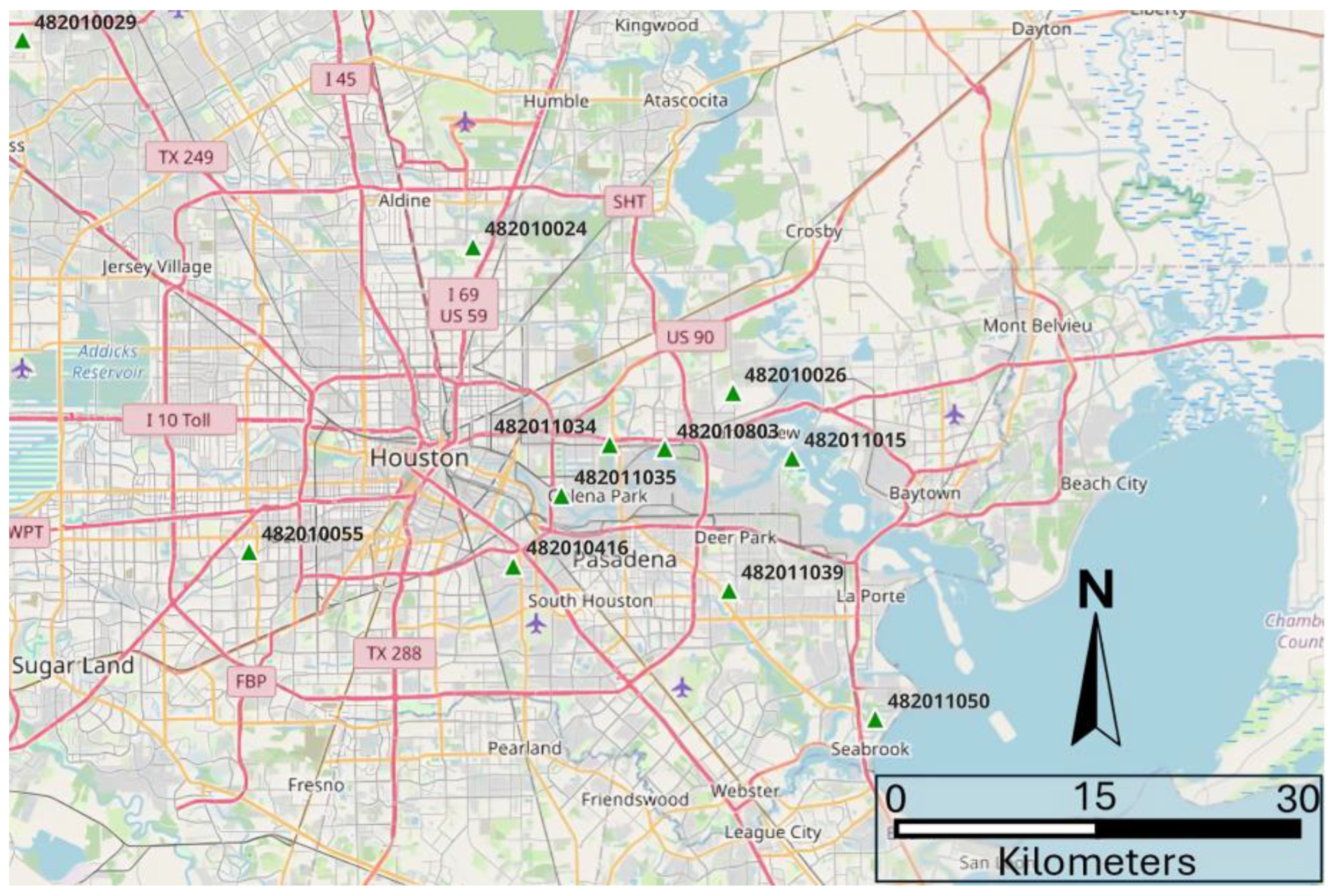
Figure 2.
The initial GNN-SAGE-QNN structure used for ozone forecasting.
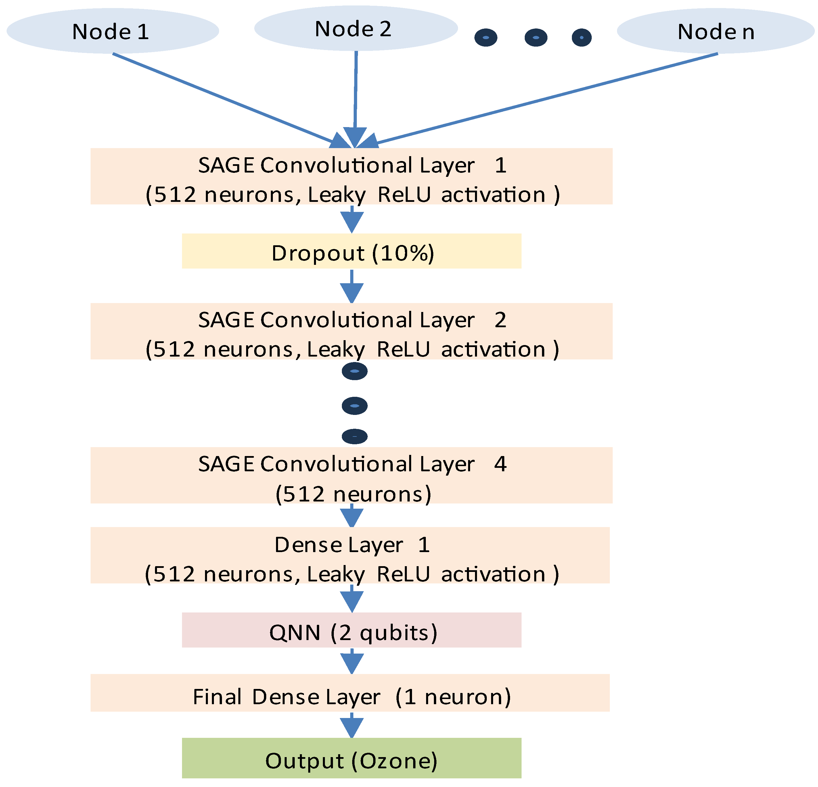
Figure 3.
The five distinct configurations for the dense layer transition from the classical to the QNN module.
Figure 3.
The five distinct configurations for the dense layer transition from the classical to the QNN module.
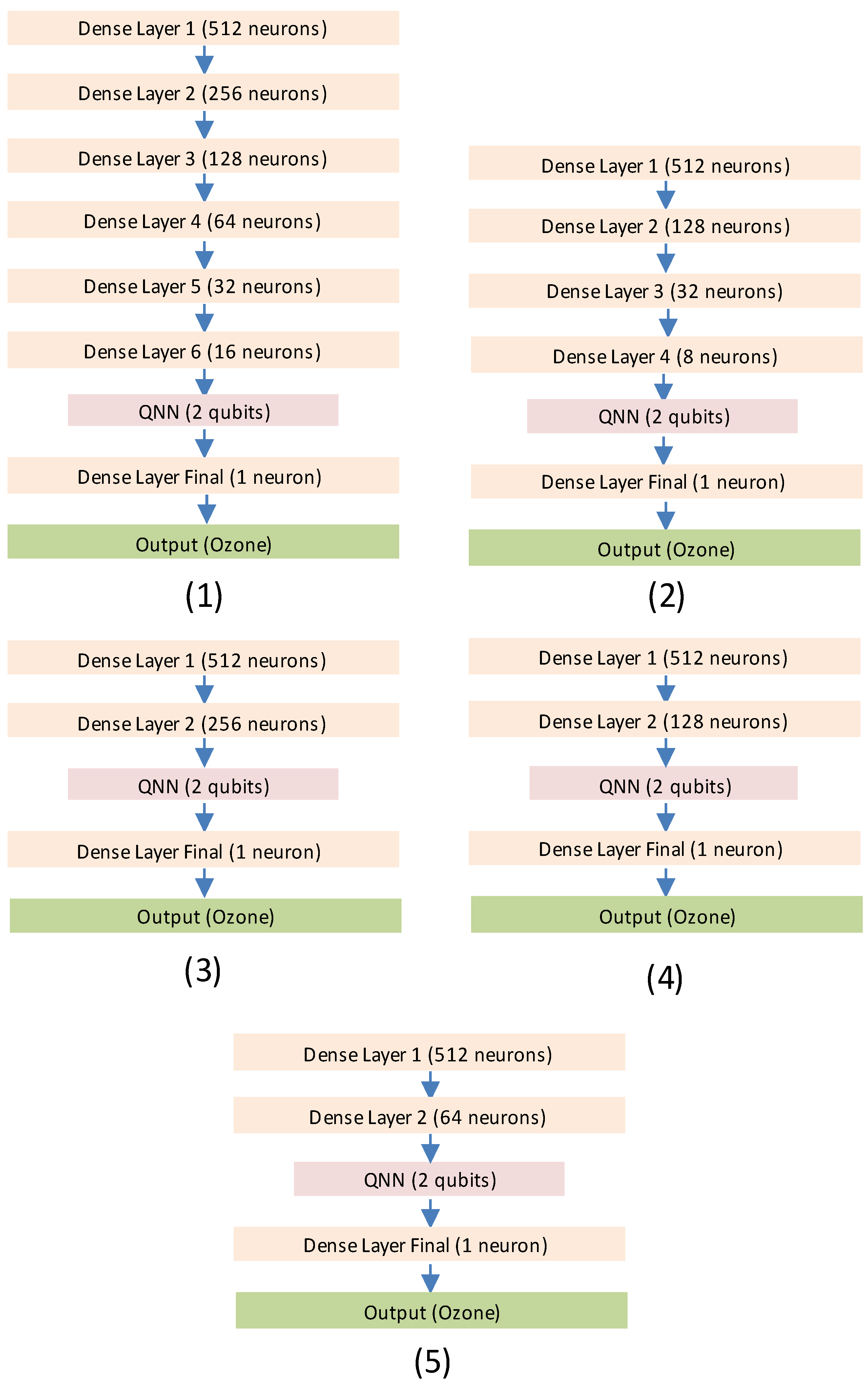
Figure 4.
Final configuration for the GNN-SAGE-QNN model for ozone concentration forecasting.
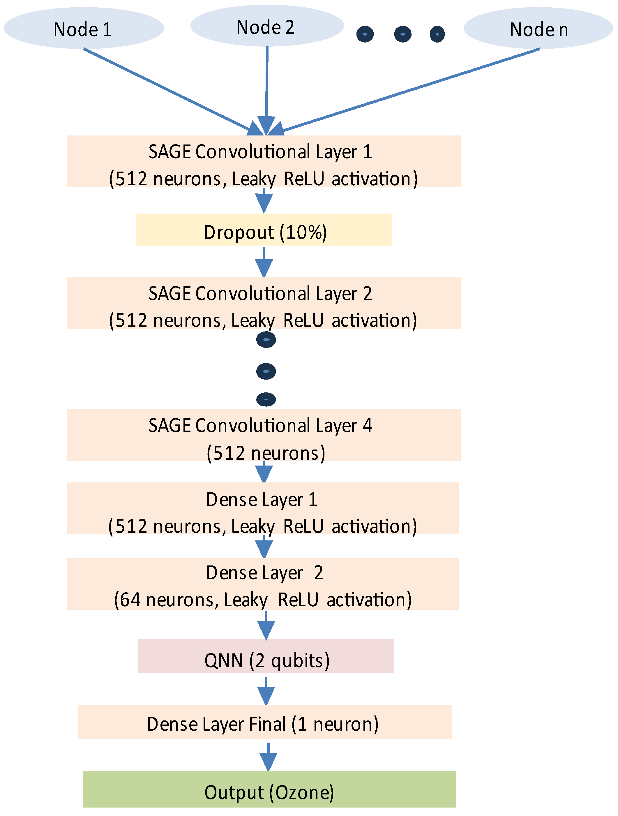
Figure 5.
Scatter plot for the 6-hour forecasting horizon using z-score normalization, one ansatz repetition and the topology depicted in Figure 4.
Figure 5.
Scatter plot for the 6-hour forecasting horizon using z-score normalization, one ansatz repetition and the topology depicted in Figure 4.
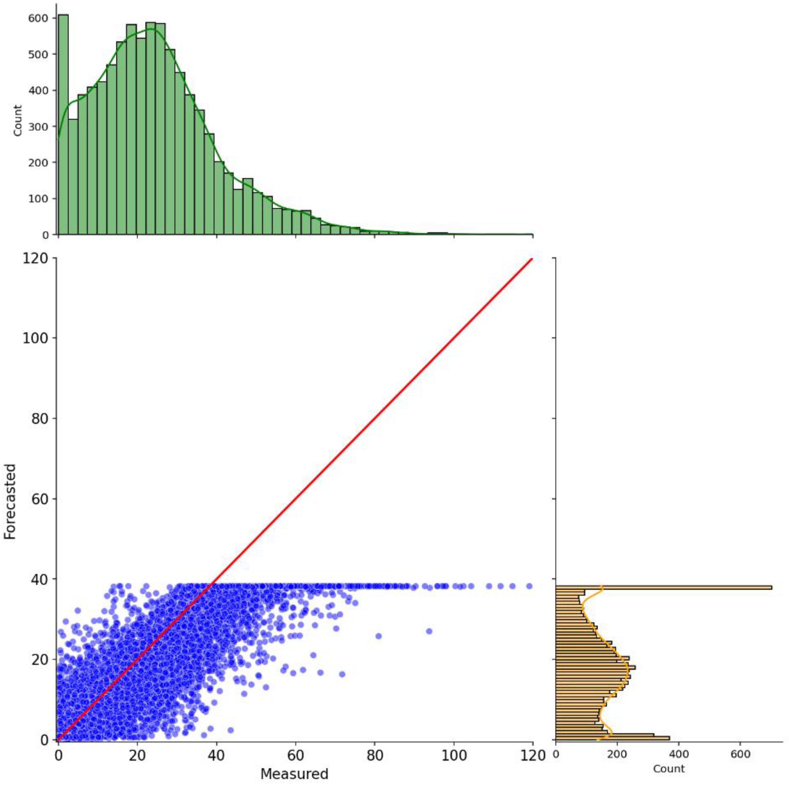
Figure 6.
Time-series comparison between the predicted and measured ozone levels 6-hour ahead for a specific period using z-score normalization, one ansatz repetition and the topology depicted in Figure 4.
Figure 6.
Time-series comparison between the predicted and measured ozone levels 6-hour ahead for a specific period using z-score normalization, one ansatz repetition and the topology depicted in Figure 4.
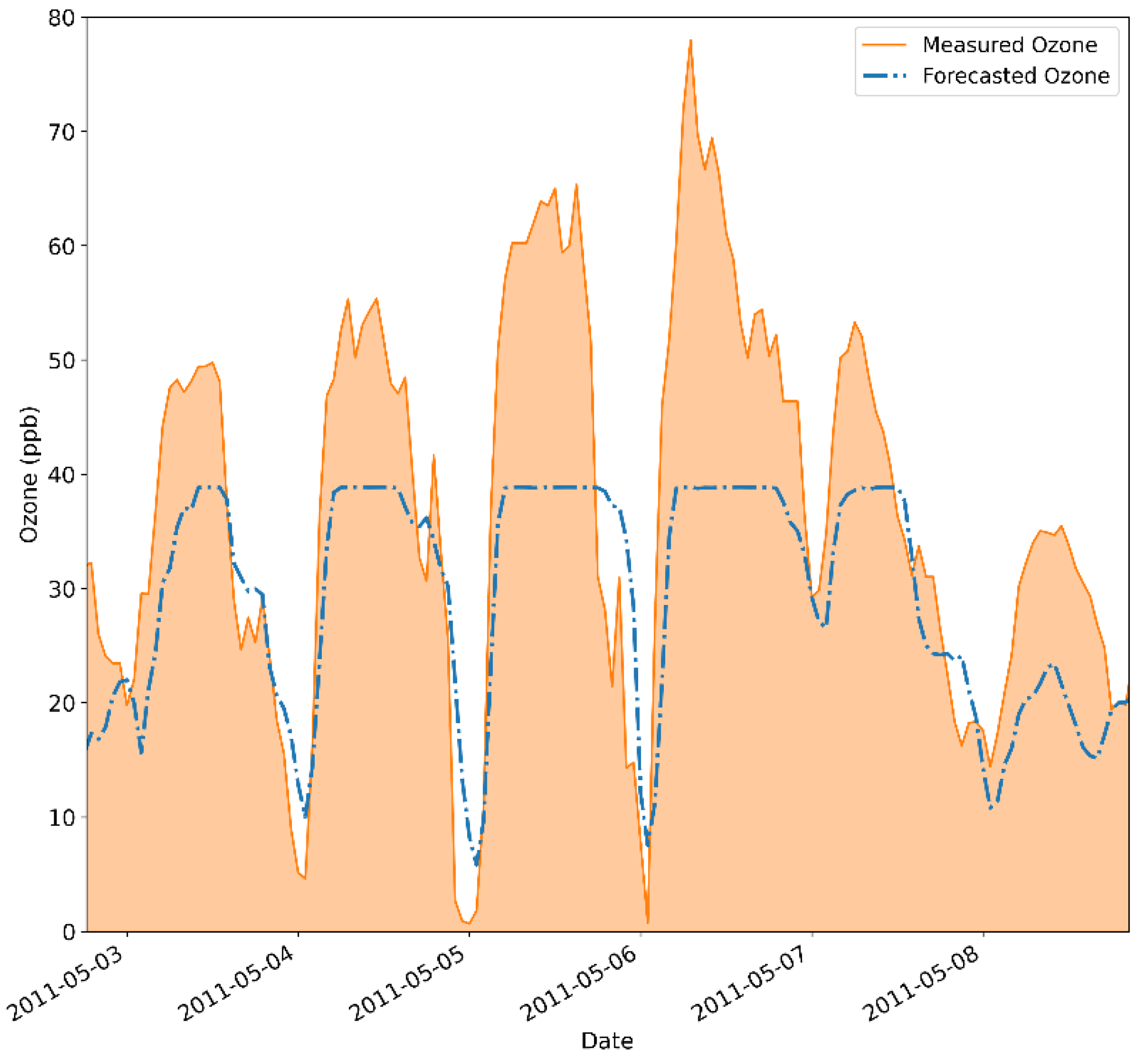
Figure 7.
Scatter plot for the 6-hour forecasting horizon using min-max normalization, one ansatz repetition and the topology depicted on Figure 4.
Figure 7.
Scatter plot for the 6-hour forecasting horizon using min-max normalization, one ansatz repetition and the topology depicted on Figure 4.
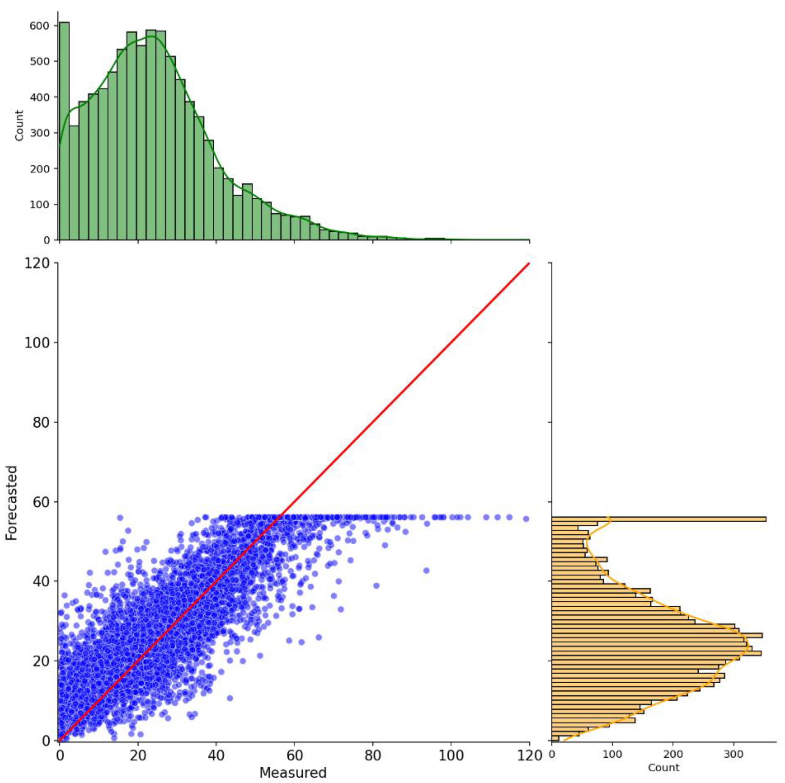
Figure 8.
Time-series comparison between the predicted and measured ozone levels 6-hour ahead for a specific period using min-max normalization, one ansatz repetition and the topology depicted on Figure 4.
Figure 8.
Time-series comparison between the predicted and measured ozone levels 6-hour ahead for a specific period using min-max normalization, one ansatz repetition and the topology depicted on Figure 4.
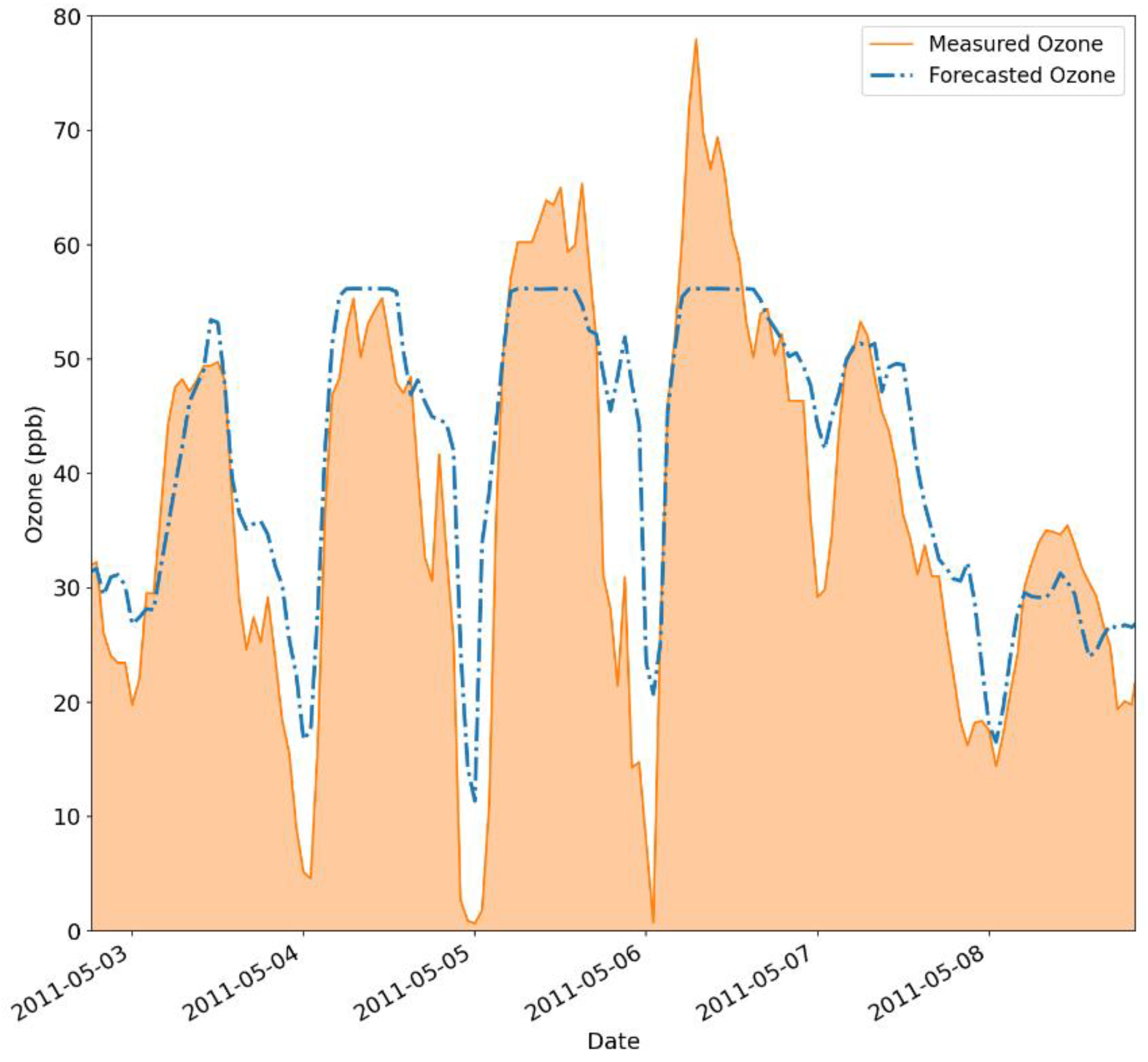
Figure 9.
Scatter plot for the 6-hour forecasting horizon using z-score normalization, two ansatz repetition and the topology depicted on Figure 4.
Figure 9.
Scatter plot for the 6-hour forecasting horizon using z-score normalization, two ansatz repetition and the topology depicted on Figure 4.
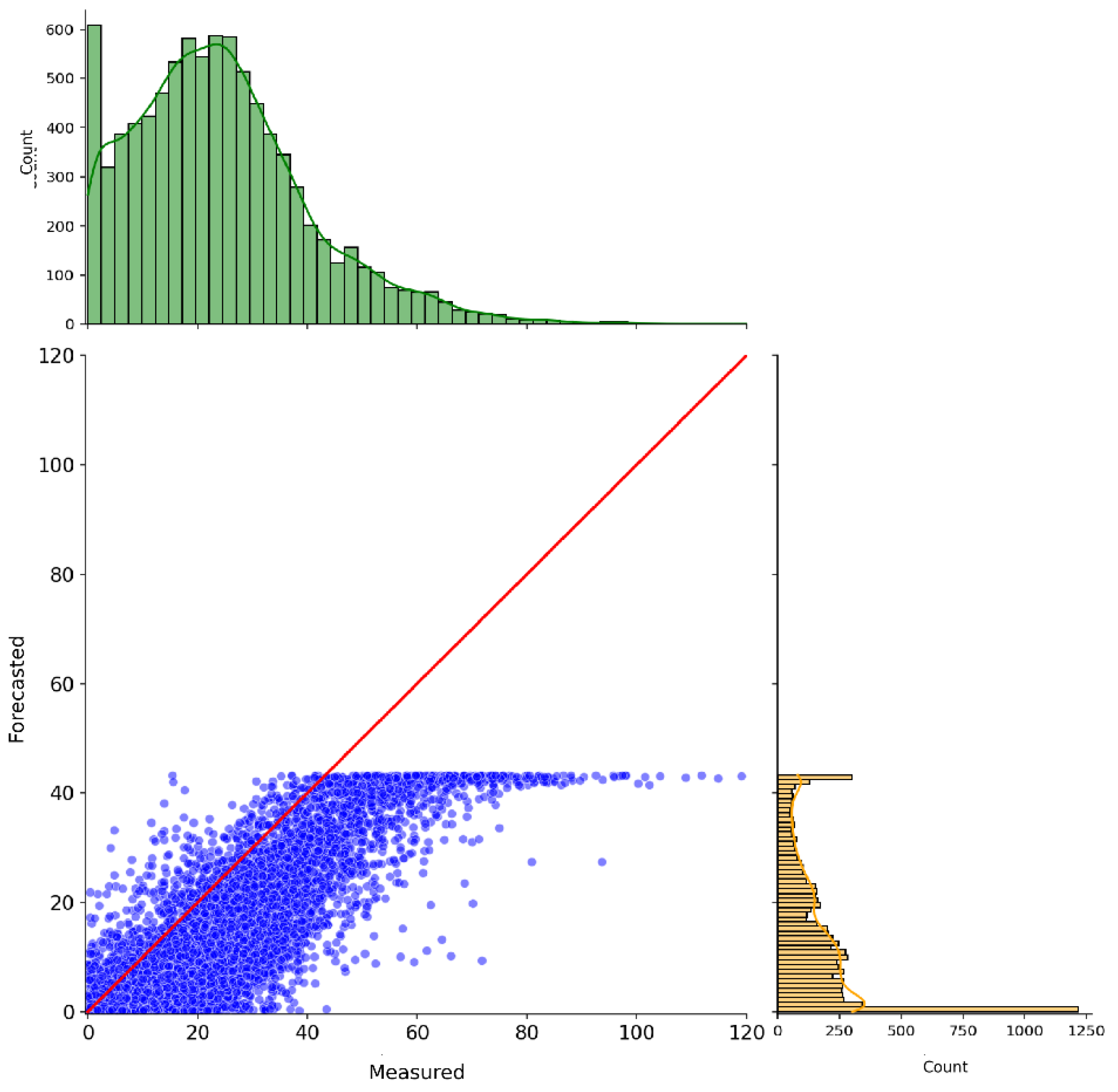
Figure 10.
Time-series comparison between the predicted and measured ozone levels 6 hours ahead for a specific period using z-score normalization, two ansatz repetition and the topology depicted on Figure 4.
Figure 10.
Time-series comparison between the predicted and measured ozone levels 6 hours ahead for a specific period using z-score normalization, two ansatz repetition and the topology depicted on Figure 4.
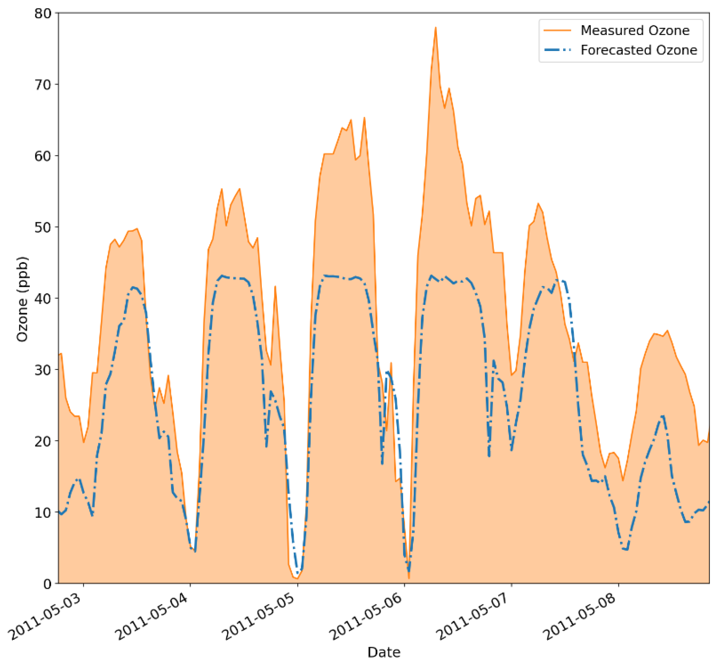
Figure 11.
Scatter plot for the 1-hour forecasting horizon using min-max normalization, three ansatz repetition and the topology depicted on Figure 4.
Figure 11.
Scatter plot for the 1-hour forecasting horizon using min-max normalization, three ansatz repetition and the topology depicted on Figure 4.
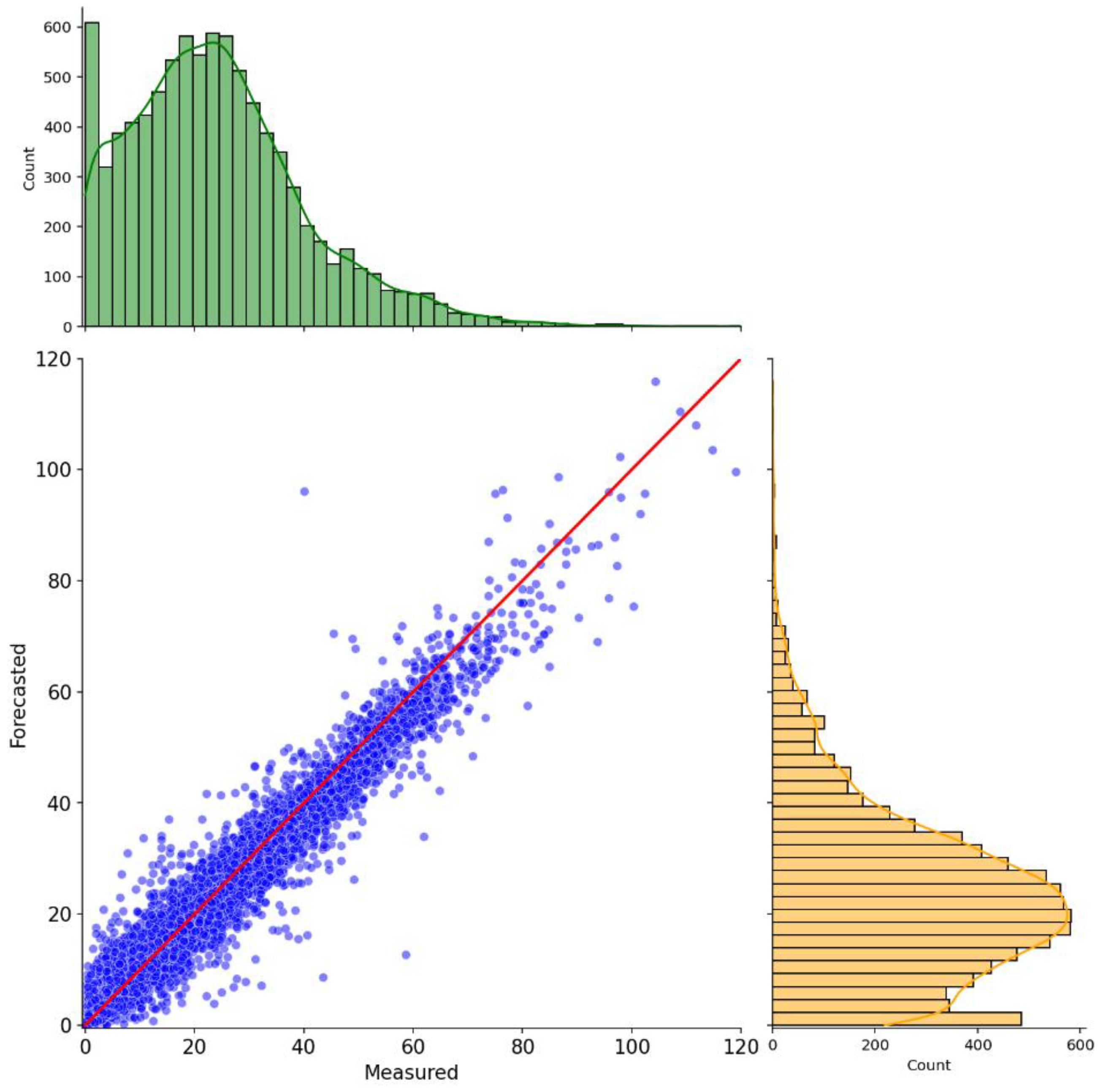
Figure 12.
Time-series comparison between the predicted and measured ozone levels 1-hour ahead for a specific period using min-max normalization, three ansatz repetition and the topology depicted on Figure 4.
Figure 12.
Time-series comparison between the predicted and measured ozone levels 1-hour ahead for a specific period using min-max normalization, three ansatz repetition and the topology depicted on Figure 4.
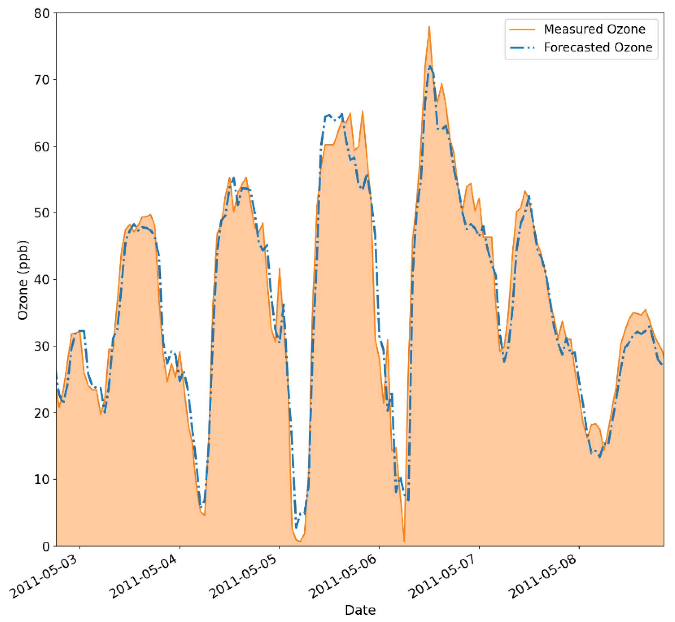
Figure 13.
Scatter plot for the 3-hour forecasting horizon using min-max normalization, two ansatz repetition and the topology depicted in Figure 4.
Figure 13.
Scatter plot for the 3-hour forecasting horizon using min-max normalization, two ansatz repetition and the topology depicted in Figure 4.
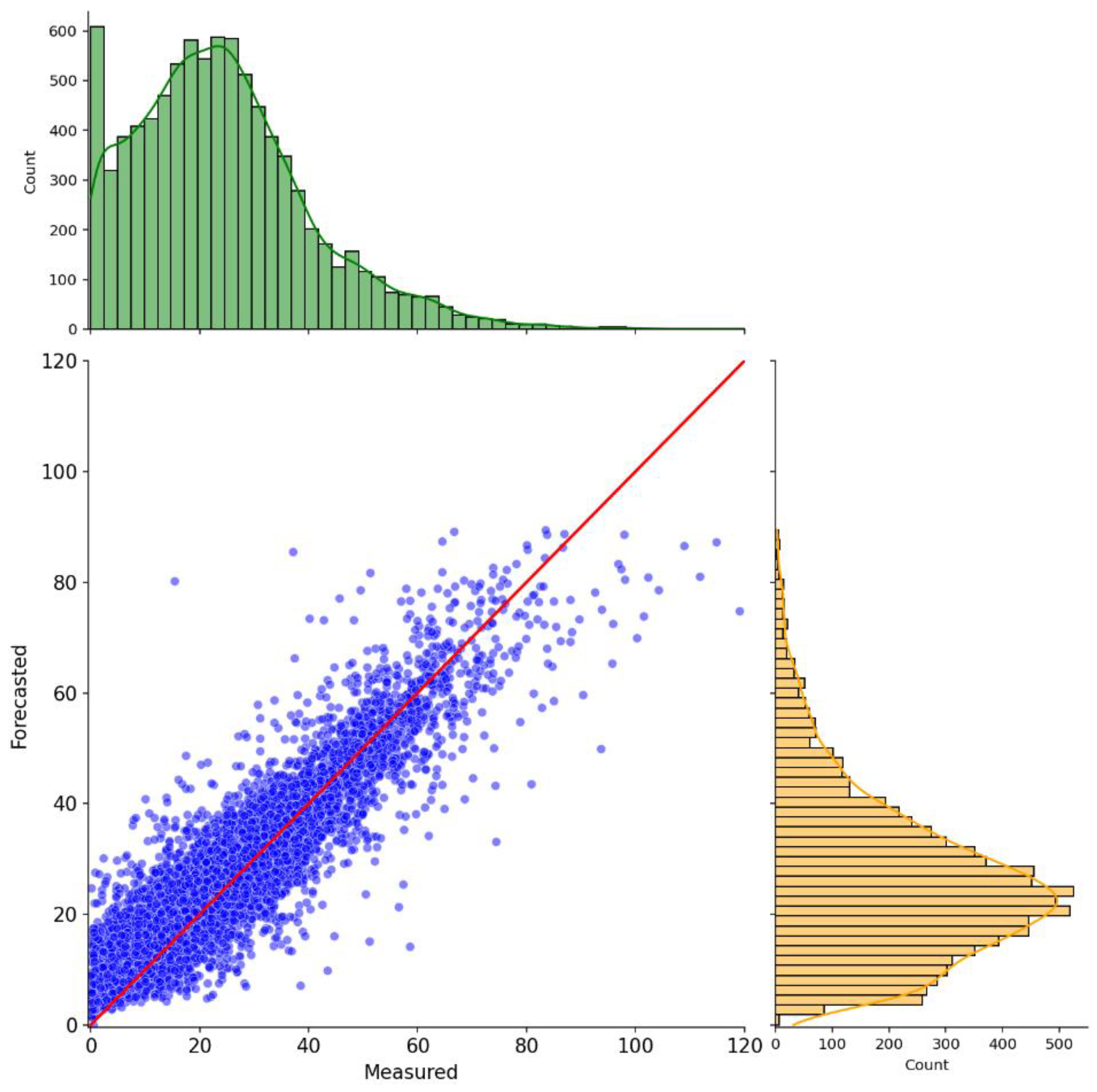
Figure 14.
Time-series comparison between the predicted and measured ozone levels 1 hour ahead for a specific period using min-max normalization, two ansatz repetition and the topology depicted in Figure 4.
Figure 14.
Time-series comparison between the predicted and measured ozone levels 1 hour ahead for a specific period using min-max normalization, two ansatz repetition and the topology depicted in Figure 4.
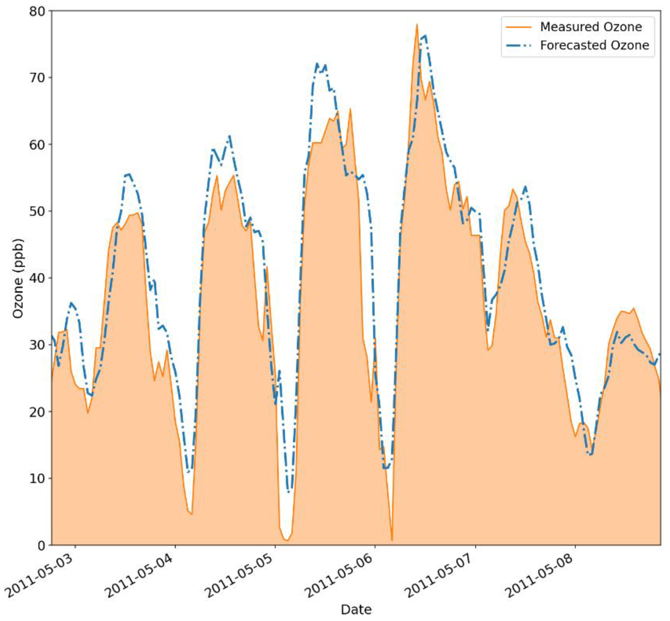
Figure 15.
Scatter plot for the 6-hour forecasting horizon using min-max normalization, two ansatz repetition and the topology depicted in Figure 4.
Figure 15.
Scatter plot for the 6-hour forecasting horizon using min-max normalization, two ansatz repetition and the topology depicted in Figure 4.
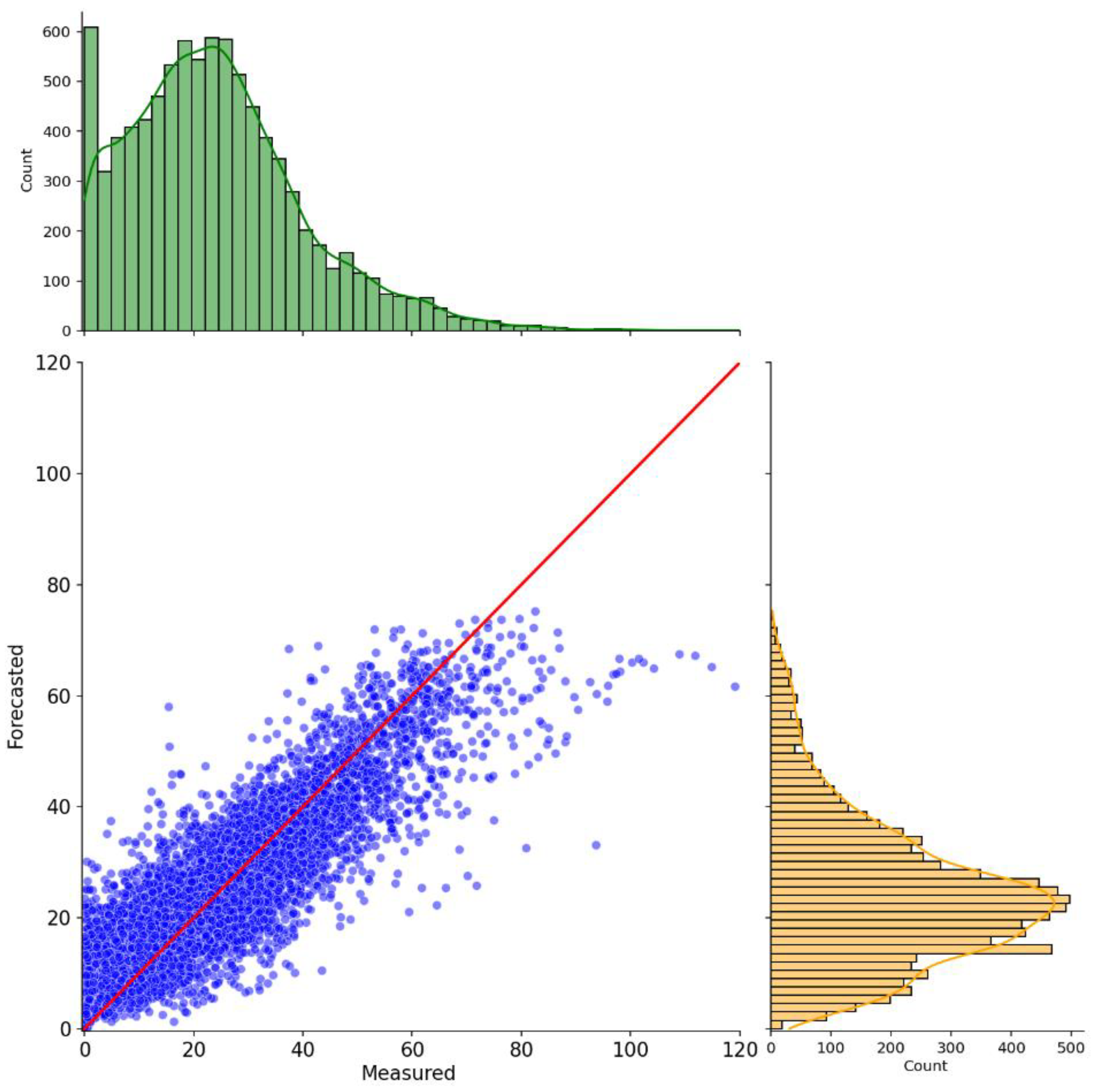
Figure 16.
Time-series comparison between the predicted and measured ozone levels 6 hours ahead for a specific period using min-max normalization, two ansatz repetition and the topology depicted in Figure 4.
Figure 16.
Time-series comparison between the predicted and measured ozone levels 6 hours ahead for a specific period using min-max normalization, two ansatz repetition and the topology depicted in Figure 4.
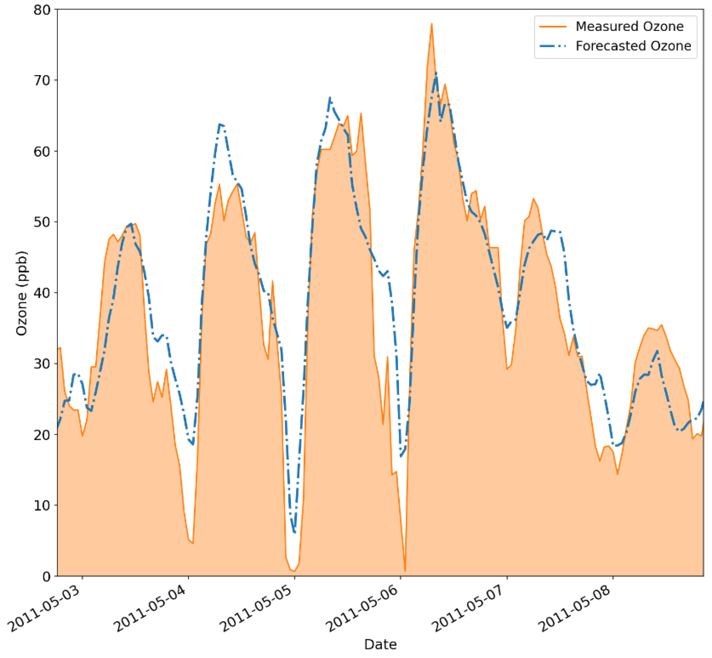

Table 1.
QNN structured used in the proposed GNN-SAGE-QNN model.
| QNN Component |
Used Approach |
|---|---|
| Feature Map | Pauli Y angle encoding |
| Ansatz | TwoLocal ansatz, with linear entanglement |
| Ansatz Optimization | L-BFGS-B |
Table 2.
Discrimination of predictors for each forecasting horizon and their respective time lags.
| Forecasting Window |
Predictors | Time-lag |
|
1 hour |
|
4 hours |
|
3 hours |
2 hours |
|
|
6 hours |
7 hours |
Table 3.
Qiskit software version.
| Qiskit Software | Version |
|---|---|
| qiskit | 1.0.2 |
| qiskit-algorithms | 0.3.0 |
| qiskit-machine-learning | 0.7.2 |
Table 4.
Results for the hybrid GNN-SAGE-QNN model using the initial structure presented in Figure 2.
Table 4.
Results for the hybrid GNN-SAGE-QNN model using the initial structure presented in Figure 2.
| Forecasting Horizon |
RMSE (ppb) |
R2 (%) |
FS (%) |
| 1 hour | 7.61 | 78.24 | -32.53 |
| 3 hours | 10.36 | 59.62 | 17.64 |
| 6 hours | 9.33 | 67.18 | 50.65 |
Table 5.
Outcomes for the different transition configurations between the dense layers and the QNN module.
Table 5.
Outcomes for the different transition configurations between the dense layers and the QNN module.
| Approach | RMSE (ppb) |
R2 (%) |
FS (%) |
| 1 | 9.11 | 68.75 | -58.80 |
| 2 | 6.31 | 85.02 | -9.97 |
| 3 | 7.63 | 78.13 | -32.86 |
| 4 | 5.58 | 88.28 | 2.75 |
| 5 | 5.50 | 88.60 | 4.10 |
Table 6.
Results for ozone levels forecasting for each prediction window using z-score normalization and one ansatz repetition.
Table 6.
Results for ozone levels forecasting for each prediction window using z-score normalization and one ansatz repetition.
| Forecasting Horizon | RMSE (ppb) |
R2 (%) |
FS (%) |
| 1-hour | 5.50 | 88.61 | 4.11 |
| 3-hour | 8.10 | 75.36 | 35.66 |
| 6-hour | 9.43 | 66.53 | 50.16 |
Table 7.
Final configuration for the hybrid GNN-SAGE-QNN model for each forecasting horizon.
| Forecasting Horizon |
Normalization | Number of Ansatz repetition |
| 1-hour | Min-max | 3 |
| 3-hour | Min-max | 2 |
| 6-hour | Min-max | 2 |
Table 8.
The outcomes for the evaluated forecasting horizons using the selected topology (Figure 4), min-max normalization and increased number of ansatz repetitions.
Table 8.
The outcomes for the evaluated forecasting horizons using the selected topology (Figure 4), min-max normalization and increased number of ansatz repetitions.
| Forecasting Horizon |
RMSE (ppb) |
R2 (%) |
FS (%) |
| 1-hour | 3.96 | 94.12 | 31.01 |
| 3-hour | 6.53 | 83.94 | 48.01 |
| 6-hour | 8.01 | 75.62 | 57.46 |
Table 9.
Literature found values for ozone forecasting for different predictive models.
| Model | Metric Value | Author |
| GNN-SAGE | RMSE – R2 – FS 3.80 ppb – 0.95% – 33.70% for 1 h horizon 6.45 ppb – 0.84% – 48.70% for 3 h horizon 8.09 ppb – 0.75% – 57.10% for 6 h horizon |
[51] |
| LSTM-based deep learning model | RMSE – R2 7.50 ppb – 83.69% for 1 h horizon |
[125] |
| Attention-based deep learning model | RMSE 2.92 ppb for 1 h horizon |
[49] |
| Transformer-based deep learning model | RMSE – R2 3.99 ppb – 92.20% for 1 h horizon 5.35 ppb – 86.31% for 3 h horizon |
[126] |
| Several classical ML models, where the SVM emerged as the best performing approach | RMSE – R2 9.24 ppb – 85.00% for 1 h horizon 14.01 ppb – 65.50% for 3 h horizon 17.70 ppb – 45.10% for 6 h horizon |
[127] |
Disclaimer/Publisher’s Note: The statements, opinions and data contained in all publications are solely those of the individual author(s) and contributor(s) and not of MDPI and/or the editor(s). MDPI and/or the editor(s) disclaim responsibility for any injury to people or property resulting from any ideas, methods, instructions or products referred to in the content. |
© 2025 by the authors. Licensee MDPI, Basel, Switzerland. This article is an open access article distributed under the terms and conditions of the Creative Commons Attribution (CC BY) license (http://creativecommons.org/licenses/by/4.0/).
Copyright: This open access article is published under a Creative Commons CC BY 4.0 license, which permit the free download, distribution, and reuse, provided that the author and preprint are cited in any reuse.


