Investigating the Possibility of Integrating Quantum Mechanics with General Relativity Through a Novel Way of Treating Time

1. Introduction

In the present work we will explore a new approach to modelling time in reference to space which diverges from the usual approaches. In our approach, time is not a fixed dimension which is experienced in the same way for all other dimensions, which are spatial. We model time by making it “dynamical” in nature, in the sense that it is neither fixed nor the same for different dimensional phenomena. Our time will always be the plus one dimension to the spatial dimensions our phenomena interact and propagate. For a phenomenon that propagates and interacts in 3 dimensions, time is the usual 4th dimension. For a phenomenon that propagates and interacts in 4 dimensions, time will be an extra 5th dimension and for this phenomenon the 4th dimension will behave as space together with the other 3 spatial dimensions of the lower dimensional phenomena. All spatial dimensions are indistinguishable from each other and behave in the exact same way (no spatial dimension is more important or different than the other). The important parameter is not the dimension we are studying (for example the 4th or the 5th) but the number of dimensions. In such an approach, time for one phenomenon can act as space for a higher dimensional one. This may appear confusing at first and may seem prone to chaotic behaviors, but when a set of rules is applied to such a dynamic multi-dimensional spacetime framework we observe that some of the predictions of both quantum mechanics and general relativity seem to arise naturally, which in turn gives us a means to integrate mathematical tools from both theories which previously were considered incompatible with each other.

In the following sections we will try to clarify the key characteristics of a time dimension for the purpose of generalizing those characteristics according to our framework. Following that, we will focus on how a higher dimensional wave would propagate in this framework and explore how a mass term arises from such a wave, the connection with the Einstein Energy Equation and how the metric tensor seems to integrate in our framework. Then, we will investigate the possible ways such a wave may interact or interfere with itself and other waves and how this would appear to us, the 3 + 1 dimensional observer. Through this we will understand why observables and complex functions would be necessary for describing such waves and why the results would appear probabilistic, with us being able only to describe correlations between them. Furthermore, we will try to derive our first most simple equation for a wave of a non-interactive scalar 4 + 1 dimensional field and compare our results with the Klein – Gordon equation and the mass term derived earlier. Lastly, we will investigate the testability of our framework by exploring possible implications it would have in our 3 + 1 dimensional frame of reference, compare some our assumptions with experimental results and examine how further experiments may validate some crucial aspects of our framework.

2. Characteristic Functions of a Time Dimension and How to Generalize Them: Connection with Entropy and Energy Dispersion

In order to better comprehend the role that a time dimension plays in our understanding and modelling of the physical world around us, we will start by examining the effects that a time dimension has on a periodic function.

We start with the usual 3 - dimensional wave of the form:

$$\mathsf{\Psi }=\mathrm{A}\sin (\omega t-k_{x}x-k_{y}y-k_{z}z)$$

(1)

where $\overrightarrow{k}$ =$\left[\begin{array}{c}{k}_x\\ k_y\\ k_z\end{array}\right]$ (1A), ${\displaystyle \frac{\omega }{\sqrt{({k_x}^2+{k_y}^2+{k_z}^2)}}}$= $u$ (1B)

(A is the amplitude of the wave, ω is the angular frequency, $\overrightarrow{k}$ is the wave vector, $u$is the velocity of the wave)

In such a wave the time dimension (symbolized by t) is vital for performing two functions:

1)

It propagates the wave (or more accurately the wave front) in space with speed $u$ in the direction of $\overrightarrow{k}$.

2)

If we focus on a specific point in space (for example $\overrightarrow{x}$ = ($\begin{array}{ccc}{x}_1,& y_1,& z_1\end{array})$), the amplitude A of that point oscillates with time with frequency f = ω/2π.

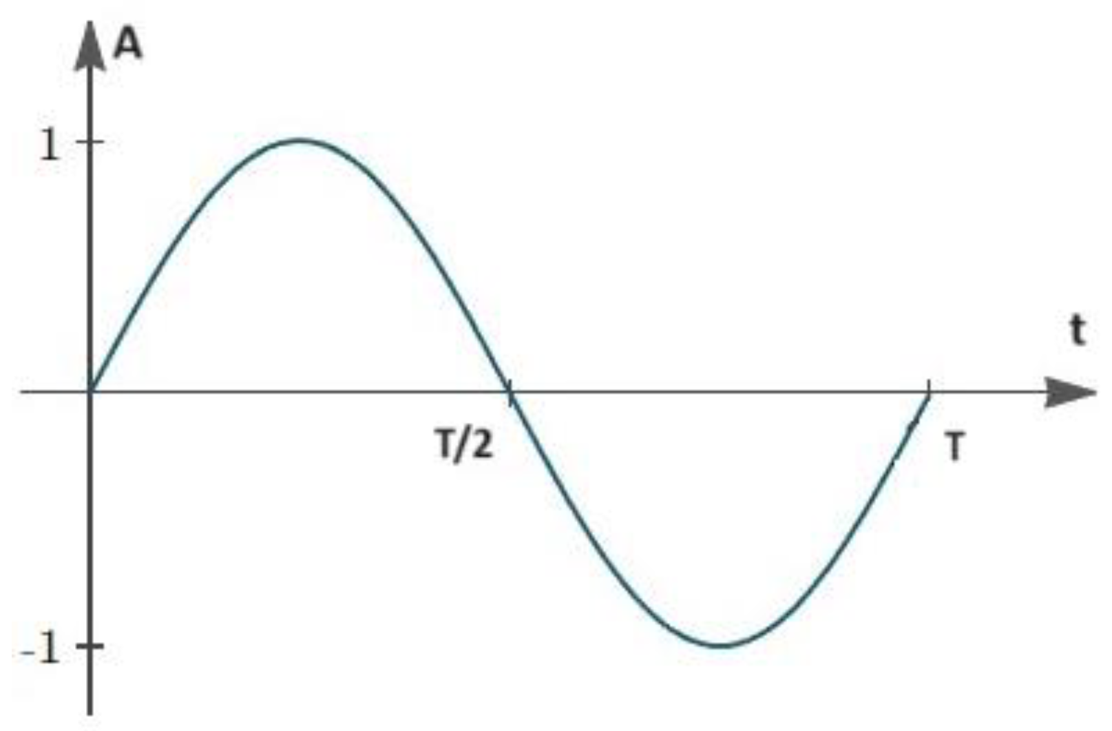
Figure 1. How the Amplitude of a 3-dimensional wave changes with time (Max Amplitude = 1, T = period of the wave) for a specific point in space $\overrightarrow{x}$ = ($\begin{array}{ccc}{x}_1,& y_1,& z_1\end{array})$.

Figure 1. How the Amplitude of a 3-dimensional wave changes with time (Max Amplitude = 1, T = period of the wave) for a specific point in space $\overrightarrow{x}$ = ($\begin{array}{ccc}{x}_1,& y_1,& z_1\end{array})$.

Every wave function corresponds to a wave equation which typically takes the form [2]:

$${\displaystyle \frac{{\partial }^2\phi }{{\partial t}^2}}=u^2({\displaystyle \frac{{\partial }^2\phi }{{\partial x}^2}}+{\displaystyle \frac{{\partial }^2\phi }{{\partial y}^2}}+{\displaystyle \frac{{\partial }^2\phi }{{\partial z}^2}})$$

(2)

The link between the two is the equation:

$$u=\mathrm{f} \ast \lambda$$

(3)

(λ is the wavelength of the wave, k = 2π / λ)

In order to model time in a dynamic way, as we mentioned in Section 1, we will focus on both of the characteristics shown above and try to generalize them together with a relation that connects the spatial dimensions with the temporal dimension, such as (3).

Regarding the first one, we are interested in propagation through space. In our framework, the time dimension of a lower dimensional phenomenon acts as a spatial dimension for a higher dimensional one. This means that we must always know the dimensionality of what we are trying to model and the dimensionality of the reference frame we are interested to model it in. For example, modelling a 4 + 1 dimensional wave in a 3 + 1 dimensional frame of reference. This is one of the things that sets apart our framework from other multidimensional frameworks. This means that we should always define the propagation vector with the right number of components (for example 4 components for the 4 + 1 dimensional wave) and also define a relation between these components that applies for the reference frame we are modelling it in (for a lower dimensional reference frame one of these components will behave as a time dimension, so it must be connected to the other components through a relation such as (3)). It is important to note that when modelling in a lower dimensional reference frame, all quantities and relations must be modelled in the lower dimensional observer’s time dimension together with relations that apply to that observer.

These relations are crucial for our framework because they are the link that connects spatial dimensions with the time dimension. Without them our framework would be prone to chaotic behaviors and results that do not correlate with our physical reality.

Focusing on the second characteristic, we turn our attention to a specific point in space. Here we should also be very careful of the dimensionality of what we are trying to model and the dimensionality of the reference frame we are interested to model it in. We must always take the same spatial dimensions as the spatial dimensions our interacting phenomenon has and examine how a specific value of this space changes with respect to the time dimension of the interacting phenomenon. For example, for a 4 + 1 dimensional wave the specific point in space we would study should also have 4 components and a specific value of this 4 – dimensional point should change in relation to the 5th dimension.

This may appear very confusing since a 3 + 1 dimensional observer would have no way of measuring the 5th dimension and in that observer’ s reference frame it would seem as a specific point in space in a specific point in time (4th dimension) has many values. This is why we need relations such as (3) that connect the temporal with the spatial dimensions so that our results remain consistent.

Finally, a crucial aspect of reality that our framework should uphold is causality and the speed of light. These should hold true for every reference frame of any dimensionality no matter the dimensionality of the phenomenon we are studying.

With all the above in mind, we will try to model a 4 + 1 dimensional wave in the reference frame of a 3 + 1 dimensional observer, with proper relations that connect the temporal with the spatial dimensions and correspond to the rules mentioned above.

3. Modelling the Propagation of 4+1 Dimensional Waves in Our Framework: Deriving a Mass Term, the Einstein Energy Relation and Integrating the Metric Tensor in Our Framework

In this Section we will focus our attempts on modelling the propagation of a 4 + 1 dimensional wave in the reference frame of a 3 + 1 dimensional observer.

As mentioned in the previous Section, we must always know the dimensionality of what we are trying to model and the dimensionality of the reference frame we are interested to model it in. This means that we should always define the propagation vector with the right number of components (4 components for the 4 + 1 dimensional wave). Also, since we are modelling in the reference frame of a 3 + 1 dimensional observer, all quantities and relations must be modelled in the observer’s time dimension and we should conserve all relationships that apply to the observer.

Furthermore, the 3 + 1 dimensional observer cannot measure the 5th dimensional component of a higher dimensional quantity or measure changes in that dimension. However, that does not mean that the observer does not experience effects of the interactions that relate to these components. Also, there are quantities that relate changes in the higher dimensional components to the lower dimensional ones (like frequency which expresses changes in time and is connected to spatial quantities through (3)). Since those quantities are vital to the lower dimensional observer for describing higher dimensional phenomena, it would make sense for the observer to model them as quantities that are intrinsic to that phenomenon and do not change or in other words are invariant quantities. An example of such a quantity may be a quantity that encapsulates the energy and momentum of a system which should remain a fundamental concept for ensuring physical laws’ consistency across all frames, analogous to invariant mass in general relativity [3].

Considering all the above, for a 4+1 dimensional wave, space is 4 dimensional (3 - dimensional time is part of our spatial dimensions now) and all space dimensions are equivalent and treated the exact same way, meaning that our new wave vector $\overrightarrow{k\text{'}}$must be 4 dimensional and have the form

$$\overrightarrow{k\text{'}}=\left[\begin{array}{c}{k}_t\\ k_x\\ \begin{array}{c}{k}_y\\ k_z\end{array}\end{array}\right]$$

$\overrightarrow{k\text{'}}$now has a 4 - dimensional direction, which means that the rate of transmition of that wave $\overrightarrow{u\text{'}}$ will also have a 4 - dimensional direction.

Also, we should have a relation analogous to (3) which connects the 4 spatial dimensions with the 5th time dimension. This relation should also preserve the speed of light limit.

Such a general relation could be the following:

The magnitude $\left|\overrightarrow{u\text{'}}\right|$ of the rate of transmition of all waves, no matter their dimensionality, is equal to the same number c, which is equal to the speed of light for the 3 - dimensional wave.

Applying such a relation would give us:

$$c={\displaystyle \frac{A}{\sqrt{{\left(\overrightarrow{k^{\text{'}}}\right)}^2}}}$$

(4)

where $A$ is the wave’s angular frequency in the 5th dimension.

The thing that remains now is to express all the above quantities in the 3 + 1 dimensional observer’s time (our time dimension) together with relations that apply to that observer (relations also expressed in our time dimension).

As we mentioned before, both quantities c and A express changes in the 5th dimension, so it would make sense for the 3 + 1 dimensional observer to express them as invariant quantities.

The new wave vector $\overrightarrow{k\text{'}}$ is a quantity that has real physical significance to the observer but depend on the observer’s reference frame. It has 4 components, 3 corresponding to the observer’s spatial dimensions and 1 corresponding to the observer’s time dimension. However, for a 4 + 1 dimensional phenomenon, the observer’s time dimension behaves as space. This means that we must express all the components of this vector with the same units and utilize the correct relations in order to express the magnitude of that vector. The solution is something that is very common in modern physics:

$$\sqrt{({k_t}^2+{k_x}^2+{{ k}_y}^2+{k_z}^2)}$$

in the 4+1 dimensional frame of reference, would be modelled as

$$\sqrt{{\displaystyle \frac{{\omega }^2}{c^2}}-{k_x}^2-{{ k}_y}^2-{k_z}^2}$$

(5)

in the 3 + 1 dimensional reference frame.

The minus sign is utilized because since both A and c remain constant in our approach, the quantity $\sqrt{{\left(\overrightarrow{k^{\text{'}}}\right)}^2}$ should also remain constant. This means that any change in magnitude of any of the components would correspond to an opposite change in some other component. Since the 3 + 1 dimensional observer experiences the 4th dimension as time it would make sense to model the 4th dimension differently and “group” those changes (that should always cancel each other out) as changes in the observer’s space and changes in the observer’s time.

Alternatively, in the formalism of vector analysis all this can be expressed as:

$$\left|\overrightarrow{k^{\text{'}}}\right|=\sqrt{{\left(\overrightarrow{k^{\text{'}}}\right)}^2}=$$

$$\sqrt{g^{\mu \nu }{k}_{\mu }{k}_{\nu }}=$$

$$\sqrt{{\displaystyle \frac{{\omega }^2}{c^2}}-{k_x}^2-{{ k}_y}^2-{k_z}^2}$$

At this point we see how the use of the metric tensor can be integrated in our framework.

Combining (4) and (5) we get:

$$c={\displaystyle \frac{A}{\sqrt{(\frac{{\omega }^2}{c^2}-{k_x}^2-{{ k}_y}^2-{k_z}^2)}}}$$

(6)

Taking the square of (6) in order to get rid of the square root in the denominator we get

$$c^2={\displaystyle \frac{A^2}{\frac{{\omega }^2}{c^2}-{k_x}^2-{{ k}_y}^2-{k_z}^2 }}$$

$$c^2\ast ({\displaystyle \frac{{\omega }^2}{c^2}}-{k_x}^2-{{ k}_y}^2-{k_z}^2)=A^2$$

$${\omega }^2-c^2{k_x}^2-{{ c^{2}k}_y}^2-{{c^{2}k}_z}^2=A^2$$

multiplying both sides with ${\hslash }^2$ in order to get units of energy we get

$$({\hslash \omega )}^2-c^2({{\hslash k}_x)}^2-{{ c^2(\hslash k}_y)}^2-{{c^2(\hslash k}_z)}^2={(\hslash A)}^2$$

$$({hf)}^2-c^2({p_x)}^2-{{ c^2(p}_y)}^2-{{c^2(p}_z)}^2={(\hslash A)}^2$$

$$E^2-c^2({p_x)}^2-{{ c^2(p}_y)}^2-{{c^2(p}_z)}^2={(\hslash A)}^2$$

(7)

For equation (7) we have used the deBroglie relation:

$p$ = $h$/λ = $\hslash k$ and the Einstein – Planck equation: E = $hf$

which apply to all fundamental particles [4].

Comparing (7) with the Einstein energy equation:

$$E^2={(m{c}^2)}^2+c^2({p_x)}^2+{{ c^2(p}_y)}^2+{{c^2(p}_z)}^2$$

(8)

we find that every 4-dimensional wave that obeys the rules we imposed on our framework should have a property which behaves like mass and is proportional to the wave’s angular frequency in the 5th dimension noted by the letter $A$.

By relating the quantity $A$ with mass we conclude that:

$${(\hslash A)}^2={\left(m{c}^2\right)}^2 \to {\displaystyle \frac{A}{c}}=\pm {\displaystyle \frac{mc}{\hslash }}$$

(9)

Summarizing the above, we see that 4 + 1 dimensional waves in our framework exhibit a property which is identical to a mass term and is proportional to the wave’s angular frequency in the 5th dimension. Also, inserting (9) to the frequency-wavelength relation (4) produces the correct form of the Einstein energy equation.

All these indicate that 4 + 1 dimensional waves in our framework have mass and propagate in 3-dimensional space with velocities less than those of the speed of light. Also, the bigger their velocities in 3-dimensional space is, the less their velocity in the 4th dimensional time. This is derived from (6) which becomes

$$\sqrt{({\displaystyle \frac{{\omega }^2}{c^2}}-{k_x}^2-{{ k}_y}^2-{k_z}^2)}={\displaystyle \frac{A}{c}}$$

Additionally, we saw that the metric tensor arises naturally from our framework. This is important because the metric tensor is a central object in general relativity that describes the local geometry of spacetime, thus making our framework compatible with the framework of general relativity [3].

4. Describing the Behaviour of a 4 + 1 Dimensional Wave: The Need for Observables and Complex Functions

In this Section, continuing the study of the behaviour of a 4 +1 dimensional wave in our framework, we will direct our efforts toward describing how a 3 + 1 dimensional observer can model the behaviour of a quantity that changes in reference to the 5th dimension.

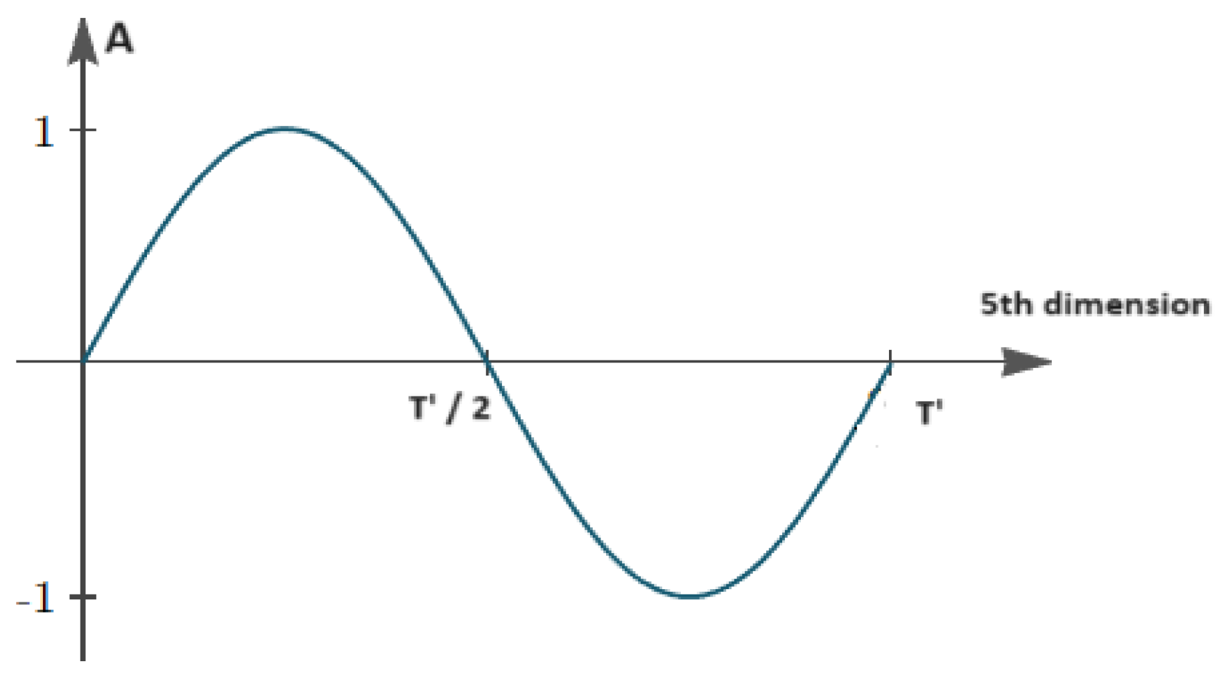
In order to do that and in accordance with Section 2, we turn our attention on a specific point in 4D space $\overrightarrow{x´}$ = ($x_1, y_1, z_1, t_1$). If the 4th dimension is treated as space, then at any such point the amplitude A of the 4th dimensional wave (not to be confused with the wave’s angular frequency in the 5th dimension which we also expressed as $A$ above) will oscillate in the 5th dimension with frequency f$\text{'}$ = ω$\text{'}$/2π.

Figure 2. How the Amplitude of a 4-dimensional wave changes in the 5th dimansion (Max Amplitude = 1, T´ = period of the wave in the 5th dimansion) for a specific point in 4D space $\overrightarrow{x´}$ = ($x_1, y_1, z_1, t_1$).

Figure 2. How the Amplitude of a 4-dimensional wave changes in the 5th dimansion (Max Amplitude = 1, T´ = period of the wave in the 5th dimansion) for a specific point in 4D space $\overrightarrow{x´}$ = ($x_1, y_1, z_1, t_1$).

This means that for a specific point in space and for a specific moment in time, as a 3D observer perceives it, a 4 - dimensional wave would seem to possess many values of A which cannot be known in advance since the observer doesn’t have access to the 5th dimension.

From the very first moment we try to mathematically model a dynamic spacetime, in the sense that we explained above, problems start to arise. More specifically, is it possible for a 3D observer to describe changes that happen in the same moment in time (4th dimension), like the Amplitude oscillation mentioned above?

In order to answer this question and start giving our dynamic spacetime a mathematical foundation, we once again turn to the 3 - dimensional wave of the form given in (1) and we ask a different question which may give us some insight into our problem. Can we model some aspects of the interactions and interferences of 3 dimensional waves without the need of time, only by using space?

Not surprisingly the answer is yes. If these waves all travel with the same speed ($u$) and all obey the equation: $u$ = f $\ast$ λ, then we can make predictions about the Amplitude of the wave on a specific point in space in correlation with its Amplitude on another point in space and also make predictions about interference patterns if we know the geometry of the sources and the relative phases of the waves [2]. This is where complex numbers come into play. For example, in a single wave if we measure the Amplitude (A₁) of the wave in one point in space we can know the amplitude (A₂) of another point at distance dx from the first point by multiplying it with a phase factor in the form:

$${\mathsf{A}}_2=\mathrm{Re}[{\displaystyle \frac{A}{A_1}}{e}^{idx\ast {\displaystyle \frac{2\pi }{\lambda }}}], \mathrm{i}=\sqrt{-1} (\mathrm{imaginary} \mathrm{unit})$$

Also, in the case of the double slit experiment for light, we know that the Amplitude of the interference pattern for any point on the screen is analogous to $e^{i\phi \left(r1\right)}$ + $e^{i\phi \left(r2\right)}$, where $r1$, $r2$ the distances of the slits from the point measured on the screen and $\phi \left(r\right)\propto$ $k\ast r$[2,9].

Figure 5. The double slit experiment and how it creates constructive and destructive interferences which have to do with the geometry of the experimental setup.

Figure 5. The double slit experiment and how it creates constructive and destructive interferences which have to do with the geometry of the experimental setup.

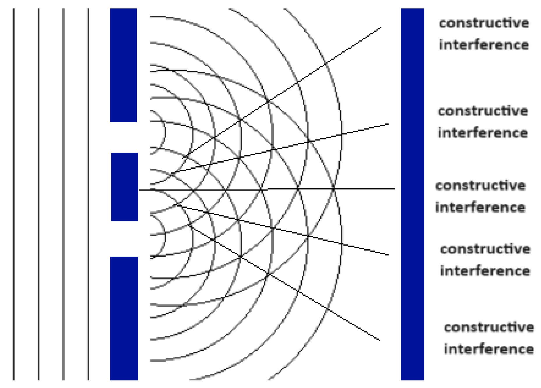
If there was an observer oblivious to the concept of our time (4th dimension) in any point of the screen of the double slit experiment, it would seem to him that the Amplitude of the wave can take many possible values. The only way any conclusion or correlation about the wave and its behavior can arise is with the use of complex numbers. Still some information is lost to the observer (like the exact value of the Amplitude because it oscillates with time, which the observer can’t measure or understand) but at least a great portion of the total information of the system would be accessible (for example if there is a constructive or destructive interference like in the double slit experiment for light).

Taking that into account, the observer who can’t understand and measure time would have to make use of complex functions and associate them with observables which the observer can measure and understand such as wavelength λ or energy (if the energy of a wave is proportional to its frequency which is the case for electromagnetic radiation – photons and free fundamental particles). Also, such waves can not be entirely described only by spatial functions (for example $\sin (\overrightarrow{k}\overrightarrow{r})$). Using the complex plane gives us a necessary extra degree of freedom, essential for our correlations.

Complex numbers are also essential for quantum mechanics. Experiments have shown that it is impossible to predict experimental results with real-number quantum theory. Also, the use of complex numbers is apparent in the fact that we can’t derive both Planck-Einstein and deBroglie relations (E=hf and p=h/λ) in quantum mechanics without their use.

A 3D wave is oscillating both in space and in time. For two different points (x₁, y₁, z₁, t₁) and (x₂, y₂, z₂, t₂), making precise correlations about the Amplitude in different times is impossible without any information about the time separation t₂-t₁. Analogous to this, if we (the 3D observer) wanted to describe a 4+1 dimensional wave and model its behaviour, the only way we could achieve this would be through the use of complex numbers, using them for correlations together with quantities measurable in the 3D plane (observables) such as distance, time separation or energy. This is where the connection with quantum mechanics in our framework starts to arise, since in quantum mechanics there is also a need for operators (which are measurable quantities) in order to determine the evolution of the quantum state and its expectation values, in reference with the values this quantum state possesses in a different point in space or in time [4,5].

Finally, we will try to give the most basic form of an equation in our framework by attempting to model a pure 4 +1 dimensional wave of a Scalar Field (Φ), which does not interact with lower dimensional disturbances of itself or any other field and propagates in a harmonic way. The magnitude of its rate of transmition is taken to be equal to the magnitude of the speed of light. For this wave the 5th dimension is acting as time and the 4th dimension (our time dimension) is acting as another spatial dimension. We are interested in modelling this wave in a way that makes sense to us, the 3 + 1 dimensional observer, following the same rules we imposed on the previous Sections.

This equation would take the form:

(Second time derivative term) = (rate of transmition)² x (second spatial derivative)

The following apply:

-

The wave is 4 + 1 dimensional which means that time for this wave is the 5th dimension

-

For this wave our time (the 4th dimension) is behaving as a spatial dimension. For this reason, our time dimension will be included in the spatial derivative terms

-

Since we are modelling the wave’s behaviour in the reference frame of a 3 + 1 dimensional observer, all quantities and relations must apply to that reference frame.

Taking all these into account our equation should have the form:

$$\mathrm{Sec}\mathrm{ond} 5\mathrm{th} \mathrm{dimensional} \mathrm{derivative} \mathrm{term}=c^2\times (\mathrm{second} \mathrm{spatial} \mathrm{derivative} \mathrm{terms})$$

(10)

$$\begin{gathered} \mathrm{Considering} \mathrm{that} \mathrm{the} \mathrm{wave} \mathrm{propagates} \mathrm{in} \mathrm{a} \mathrm{harmonic} \mathrm{way} \mathrm{in} \mathrm{the} 5\mathrm{th} \mathrm{dimension} \mathrm{and} \\ \mathrm{taking} \mathrm{a} \sin \mathrm{usoidal} \mathrm{solution} \mathsf{\Phi }, \mathrm{the} \sec \mathrm{ond} 5\mathrm{th} \mathrm{dimensional} \mathrm{derivative} \mathrm{term} \mathrm{will} \mathrm{be} \mathrm{in} \mathrm{the} \\ \mathrm{form}: {-A}^2\Phi \end{gathered}$$

(11)

(where $A$ is the wave’s angular frequency in the 5th dimension)

The second spatial derivative terms will now include 3-dimensional time (4th dimension) and we will again make use of the Minkowski metric (metric tensor for flat spacetime) because we want the results to have a physical meaning to us the 3 + 1 dimensional observer. This means that the spatial derivative terms will take the form [6]:

$$\left({\displaystyle \frac{1}{c^2}}{\displaystyle \frac{{\partial }^2}{{\partial }^{2}t}}-{\nabla }^2\right)\Phi$$

(12)

Combining (10), (11) and (12) we get:

$${-A}^2\mathsf{\Phi }=c^2\times \left({\displaystyle \frac{1}{c^2}}{\displaystyle \frac{{\partial }^2}{{\partial }^{2}t}}-{\nabla }^2\right)\Phi$$

$$\left({\displaystyle \frac{1}{c^2}}{\displaystyle \frac{{\partial }^2}{{\partial }^{2}t}}-{\nabla }^2\right)\mathsf{\Phi }+{\displaystyle \frac{A^2}{c^2}}\Phi =0$$

which is equal to the Klein – Gordon equation if we consider that:

$${\displaystyle \frac{A^2}{c^2}}={\left({\displaystyle \frac{mc}{\hslash }}\right)}^2 \to {\displaystyle \frac{A}{c}}=\pm {\displaystyle \frac{mc}{\hslash }}$$

The same result for $A$ as the one we derived earlier!

This is very promising since the mass term we derived by alternative means in Section 2 is identical to the mass related component in the Klein – Gordon and Dirac equations [7,8]:

$$\left[{\displaystyle \frac{1}{c^2}}{\displaystyle \frac{{\partial }^2}{{\partial }^{2}t}}-{\nabla }^2+{\left({\displaystyle \frac{mc}{\hslash }}\right)}^2\right]\Psi =0 (\mathrm{Klein}–\mathrm{Gordon} \mathrm{equation})$$

$${\gamma }^0{\displaystyle \frac{\partial \Psi }{c\partial t}}+{\gamma }^1{\displaystyle \frac{\partial \Psi }{\partial x}}+{\gamma }^2{\displaystyle \frac{\partial \Psi }{\partial y}}+{\gamma }^3{\displaystyle \frac{\partial \Psi }{\partial z}}+{\displaystyle \frac{mc}{\hslash }} i \Psi =0 (\mathrm{Dirac} \mathrm{equation})$$

Also, in QFT the mass term is recognized as a term in the Lagrangian that is quadratic in the field and has the form $A^2{\mathsf{\phi }}^2$ for some $A$ ($A$ ∝ m the mass of the particle) [7,8]. Since we can not exactly model the behaviour of 4+1 dimensional waves as we showed in this Section and need to make correlations with observables, such a term would make sense to appear in any attempt of the 3D observer to model the possible interactions and of those waves with themselves and other lower dimensional waves.

5. The Compatibility of Our Framework with Physical Reality and Its Testability

Considering the results of the previous Sections, we conclude that in our proposed framework all higher dimensional filed disturbances or interactions exhibit a property analogous (if not equivalent) to mass which produces the correct Einstein Energy Equation. Also, they propagate in 3-dimensional space with velocities lower than the speed of light and the more their 3D speed component approaches the speed of light the less their 4-dimesnional speed component would be. Additionally, we demonstrated that modelling exactly the behaviour of such disturbances or interactions in our 3+1 reference frame is not possible because of our lack of information regarding the 5th dimension. Instead, we can model their behaviour by making correlations with measurable, in our 3D plane, quantities and thus have a picture about interferences, dispersions and propagations.

Summarizing the above we conclude that all higher dimensional filed disturbances or interactions exhibit behaviour which is compatible with both quantum mechanics and special relativity. This compatibility should also apply to the interactions of these disturbances with lower dimensional fields or lower dimensional disturbances of themselves. Furthermore, the fact that the metric tensor arises naturally from the rules we imposed gives us a means of integrating the results of general relativity in our framework. This could for example be done by an equation that relates the metric tensor with the rate of transmition of the higher dimensional disturbance and the total energy of the system. All these demonstrate the compatibility of our framework with physical reality.

Our framework also exhibits some other aspects that are not integrated in other theories and it is these aspects that should provide us with a means of testing it.

In Section 3 we equated the 5th dimensional frequency with a term proportional to the quantity ${\displaystyle \frac{m}{\hslash }}$. In the case where a 3 + 1 dimensional wave beam is split in two, one enters a medium (where its speed decreases depending on the medium’s refractive index, but the frequency remains the same) and the other one does not and then the two beams are recombined, the interaction depends on the relative phase difference between the two beams when they recombine. The phase difference is affected by the optical path difference, which in turn depends on the frequency of the light because the refractive index of a medium is generally frequency-dependent (dispersion). Analogous to this if a 4 + 1 dimensional wave beam was split in two, the one part enters a region where its propagation would depend on the 5th dimensional frequency and the other one enters a region with different propagation - frequency dependence, when the two beams would recombine the interaction would depend on the 5th dimensional frequency of the waves which we equated to mass (9). This is in accordance with the gravity – induced quantum interference experiment in 1975 by R. Colella, A. Overhauser and S. A. Werner and their results published in Physical Rev. Lett. 34 (1975) 1472 [10], which say that the effects depend on the quantity ${\left({\displaystyle \frac{m}{\hslash }}\right)}^2$. Both beams pass through different propagation – 5th dimensional frequency (mass) dependence regions.

Furthermore, in our framework, our time dimension (4th dimension) can behave as space for a higher dimensional interaction. All spatial dimensions should behave in the exact same way and be indistinguishable from each other in the higher dimensional reference frame. This implies that there should be no restriction in the direction of motion of a higher dimensional disturbance in the 4th dimension. Taking into account that we have not considered the effects of entropy and the 2nd law of thermodynamics, which may restrict this direction of motion, experimental findings that suggest results with negative time correlation should be a strong supporter of our framework. These results should not however affect causality or provide faster than light propagation of information since it would violate the rule we imposed on Section 3. The results of recent research [11] done by a team in the University of Toronto and suggest that negative values taken by times such as the group delay have more physical significance than has generally been appreciated, may be one of those results in favor of our framework.

6. Summary

Through a novel way of modelling the time dimension we constructed a framework which allowed us to explore new ways of integrating quantum mechanics and general relativity by dynamically linking temporal and spatial dimensions, which are typically treated as distinct in these frameworks.

We demonstrated that under this framework higher dimensional filed disturbances or interactions exhibit properties analogous to mass and obey relationships consistent with the Einstein energy equation. This dynamic treatment of time also naturally incorporated the metric tensor, suggesting compatibility with general relativity. Furthermore, the probabilistic behaviour and need for observables in quantum mechanics emerged as an intrinsic feature of the framework.

The possibility of integrating some of the mathematical tools of both quantum mechanics and general relativity, in particular: Operators, Complex Functions (Wavefunctions), Probabilistic Behaviour, the Metric Tensor and the Einstein Energy Equation, offers a promising avenue for unifying quantum mechanics and general relativity, potentially solving one of the greatest problems of modern physics. Also, certain features of our framework seem to be in accordance with experimental results and we also suggested potential experimental directions to further test it.

Future research should delve into refining the mathematical foundation of this framework, investigating how interactions of higher and lower dimensional phenomena should be modelled, and exploring its compatibility with emerging experimental data. Finally, we believe that modelling the interaction of 4+1 dimensional and 3+1 dimensional fields together with imposing symmetries on them could be of much significance and possibly help better understand or more accurately produce some of the possible interactions and equations in QFT. These efforts may further validate and expand the scope of this dynamic higher-dimensional spacetime framework, bridging the gap between the two most successful theories of modern physics.

References

- Penrose, R. (2004). The Road to Reality: A Complete Guide to the Laws of the Universe. Jonathan Cape.
- Newton, R. G. Scattering Theory of Waves and Particles, 2nd ed., New York: McGraw-Hill, 1982.
- Misner, C. W., Thorne, K. S., & Wheeler, J. A. (1973). Gravitation. W. H. Freeman and Company.
- Griffiths, D. J. Introduction to Quantum Mechanics 2nd ed., Upper Saddle River, NJ: Pearson, 2005.
- J.J. Sakurai, J. Napolitano, Modern Quantum Mechanics, 2nd ed., Boston: Addison-Wesley, 2010.
- Gregory L. Naber, The Geometry of Minkowski Spacetime: An Introduction to the Mathematics of the Special Theory of Relativity. Springer-Verlag, 1992.
- M.Peskin and D.Schroder, An Introduction to Quantum Field Theory, Perseus Books, 1995.
- S.Coleman, Quantum Field Theory, World Scientific, 2019.
- Feynman R. P. and A. R. Hibbs. Quantum Mechanics and Path Integrals, New York: McGraw-Hill, 1965.
- R. Colella, A. W. Overhauser, S. A. Werner, Observation of Gravitationally Induced Quantum Interference, Phys. Rev. Lett. 34, 1472, June 1975.
- Daniela Angulo, Kyle Thompson, Vida-Michelle Nixon, Andy Jiao, Howard M. Wiseman, and Aephraim M. Steinberg1, Experimental evidence that a photon can spend a negative amount of time in an atom cloud. [CrossRef]
Disclaimer/Publisher’s Note: The statements, opinions and data contained in all publications are solely those of the individual author(s) and contributor(s) and not of MDPI and/or the editor(s). MDPI and/or the editor(s) disclaim responsibility for any injury to people or property resulting from any ideas, methods, instructions or products referred to in the content. |
© 2025 by the authors. Licensee MDPI, Basel, Switzerland. This article is an open access article distributed under the terms and conditions of the Creative Commons Attribution (CC BY) license (http://creativecommons.org/licenses/by/4.0/).
Copyright: This open access article is published under a Creative Commons CC BY 4.0 license, which permit the free download, distribution, and reuse, provided that the author and preprint are cited in any reuse.