A Framework for Iterative Phase Retrieval Technique Integration into Atmospheric Adaptive Optics. Part II: High Resolution Wavefront Control in Strong Scintillations

1. Introduction

In Part I of this two-part paper (see Ref. [1]) we provided analysis of scintillation resistant (SR) wavefront sensing architectures based on iterative phase retrieval (IPR) techniques that can potentially be applied for closed-loop wavefront control in atmospheric adaptive optics (A-AO) applications characterized by strong intensity fluctuations (scintillations) resulting from laser beam propagation over a horizontal or slant path near the ground. Among these applications are directed energy laser beam projection (DE-LBP) [2,3], remote laser power delivery (remote power beaming) [4,5] and free-space optical (FSO) communications [6,7].

Here in Part II we discuss basic A-AO system architectures characteristic for these applications in which the IPR-based SR wavefront sensing is utilized for adaptive mitigation of turbulence-induced phase aberrations. The wave-optics-based numerical simulation results presented demonstrate that the long-standing problem of AO control under strong intensity scintillations can potentially be resolved by transitioning to A-AO systems that utilize the IPR-based SR wavefront sensors (SR-WFSs) and feedback control approaches described.

Comparative performance analysis of different SR sensors – candidates for possible integration into A-AO systems – was presented in Part I through numerical modeling and simulation (M&S). It was shown that two phase-contrast type SR-WFSs, specifically the scintillation-resistant advanced phase-contrast (SAPCO) WFS and multi-aperture phase-contrast (MAPCO) sensor (Ref. [1] and Ref. [8]), have dominant performance superiority among other basic WFS types considered, and hence are the most promising for practical A-AO applications. Although both sensors exhibited nearly identical efficiency, due to simplicity of the SAPCO sensor the analysis in this paper (Part II) was narrowed down to only closed-loop AO control based on the SAPCO WFS, referred to here as SAPCO-AO control. However, as expected and assessed through M&S not presented here, analogous performance can be achieved using wavefront control based on the MAPCO WFS.

In Section 2 of this paper we introduce a generic DE-LBP system architecture utilizing SAPCO-AO control approach and discuss the corresponding mathematical model and issues characteristic for implementation of phase-conjugate (PC) type wavefront control algorithms in A-AO systems with IPR-based wavefront sensors. To primarily focus on the most essential control problems we intentionally considered an idealized model of piston-type wavefront corrector (deformable mirror, DM) composed of a densely packed array of n_DM x n_DM square mirrors (subapertures) providing independent control of subaperture-averaged (piston) phases.

For evaluation of SAPCO-AO control concept under different atmospheric turbulence and scintillation conditions the following application-specific performance measures (metrics) were considered: target-plane power-in-the-bucket (PIB) for DE-LBP, beam shape fidelity (BSF) for remote laser power beaming and power-in-the-fiber (PIF) for FSO communications. These metrics are introduced in the corresponding sections dedicated to each of these applications.

Analysis of SAPCO-AO control efficiency for DE-LBP (Section 2), remote laser power beaming (Section 3) and FSO communications (Section 4) applications was based on N_trial =100 computer simulated AO control trials. Each AO trial was composed of sequential wavefront aberration sensing and control update steps (AO control cycle steps) of equal duration τ_AO. The M&S trials were conducted using identical initial conditions and different (statistically independent) turbulence realizations represented by N_φ =20 equally spaced 2D random thin phase screens corresponding to the Kolmogorov turbulence power spectrum (as described in Part I, Ref [1]). Performance metric values computed in these AO trials were further averaged and the obtained dependencies characterizing atmospheric-averaged (or AO trial-averaged) metric evolution during AO control were utilized for SAPCO-AO control system parameter optimization and efficiency assessment under different turbulence strengths.

In numerical simulations of the DE-LBP system in Section 2 we also considered the impact of cross-wind induced effects. This analysis enables estimation of the SAPCO-AO closed-loop operational bandwidth for different turbulence strength and cross-wind speed values. The M&S methodology outlined here and described in more detail in Section 2 was applied for performance evaluation of SAPCO-AO control in the A-AO applications mentioned above.

Remote laser power transfer in a turbulent atmosphere with SAPCO-AO-based beam shaping is discussed in Section 3. The adaptive wavefront control problem is formulated in terms of minimization of the beam shape fidelity metric characterizing “closeness” of the target-plane intensity distribution to the desired (reference) 2D intensity profile associated with a specific shape of the power beaming receiver, e.g., a square densely packed array of photovoltaic cells (PVCs). It is shown that minimization of the beam shape fidelity metric can be achieved via conjugation of the wavefront phase of the received optical wave originating from a specially designed (pre-shaped) laser beacon beam, referred to here as a PS-beacon whose 2D intensity profile (shape) is defined by the laser power beaming receiver geometry. The introduced adaptive beam shaping technique was evaluated through M&S by considering remote laser power delivery onto different sizes of square shaped PVC receivers (PVC-targets) under different turbulence conditions. Numerical analysis demonstrates the capabilities and limitations of the proposed control approach to shape the transmitted laser beam intensity distribution onto the target shape in order to increase the amount of delivered laser power and reduce the level of turbulence-induced scintillations and intensity spikes inside the receiver area.

In Section 4 we consider the application of the SAPCO-AO control system architecture and adaptive beam shaping technique for performance enhancement of bidirectional FSO communication links utilizing single-mode fibers (SMFs) for both laser beam transmission and received light power (power-in-the-fiber, PIF) measurements. It was shown that wavefront control in FSO communication links leading to PIF metric maximization can be considered as a derivative of adaptive beam shaping control as described in Section 3, in which the PS-beacon beam having characteristics desired for PIF metric maximization coincides with the laser beam transmitted by the remotely located FSO communication terminal. M&S of the SAPCO-AO-based bidirectional FSO links were conducted for propagation distances ranging from 0.5 km to 10 km, and different turbulence strengths and piston DM resolutions (parameter n_DM). Numerical simulations show that within the system parameter space considered in Section 4 adaptive beam shaping applied at a single FSO terminal resulted in a significant increase in received laser power coupling into the SMFs at both FSO communication terminals and a corresponding maximization of the received PIF signal.

In the concluding remarks (Section 5) we discuss both the potentials for and challenges of implementing IPR-based SR wavefront sensing and control techniques for A-AO applications.

2. Laser Beam Projection in a Turbulent Atmosphere with SAPCO-AO Control

2.1. Control System Architecture

The AO wavefront control objective in DE-LBP application is the achievement and maintenance the highest possible laser power density within the vicinity of a pre-selected point (aimpoint) at a remotely located target via adaptive shaping (control) of the transmitted laser beam wavefront phase $u(r,t)$ [2,9]. Here $r=\{x,y\}$ and t are, correspondingly, the coordinate vector at the DE-LBP system transceiver telescope (beam director, BD) pupil plane and time.

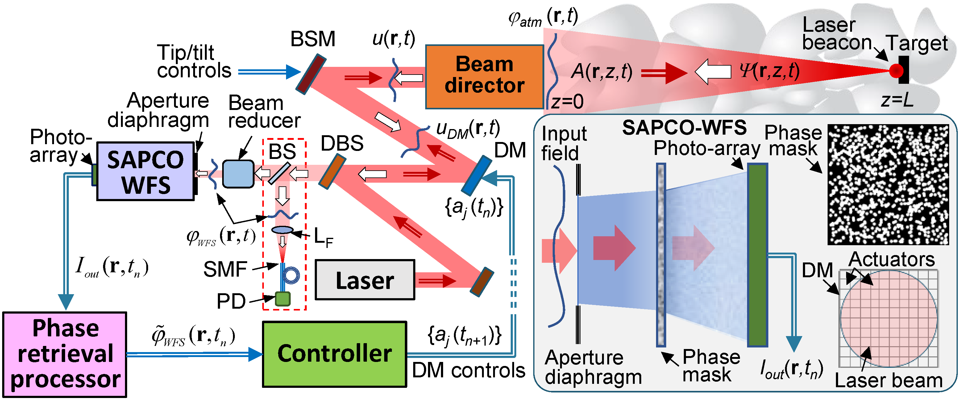
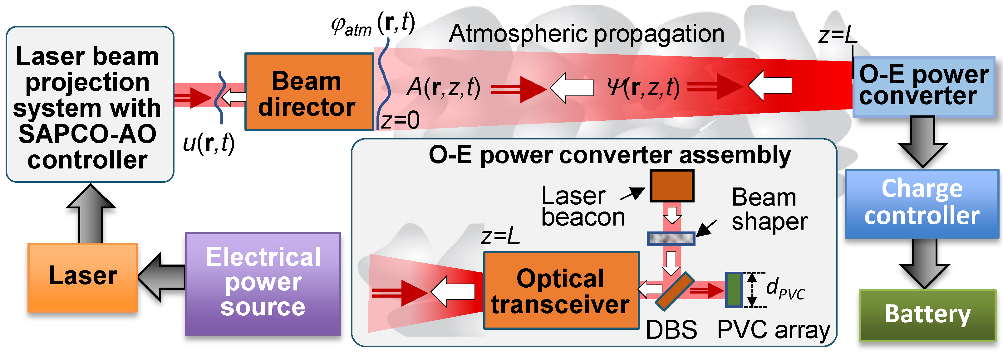
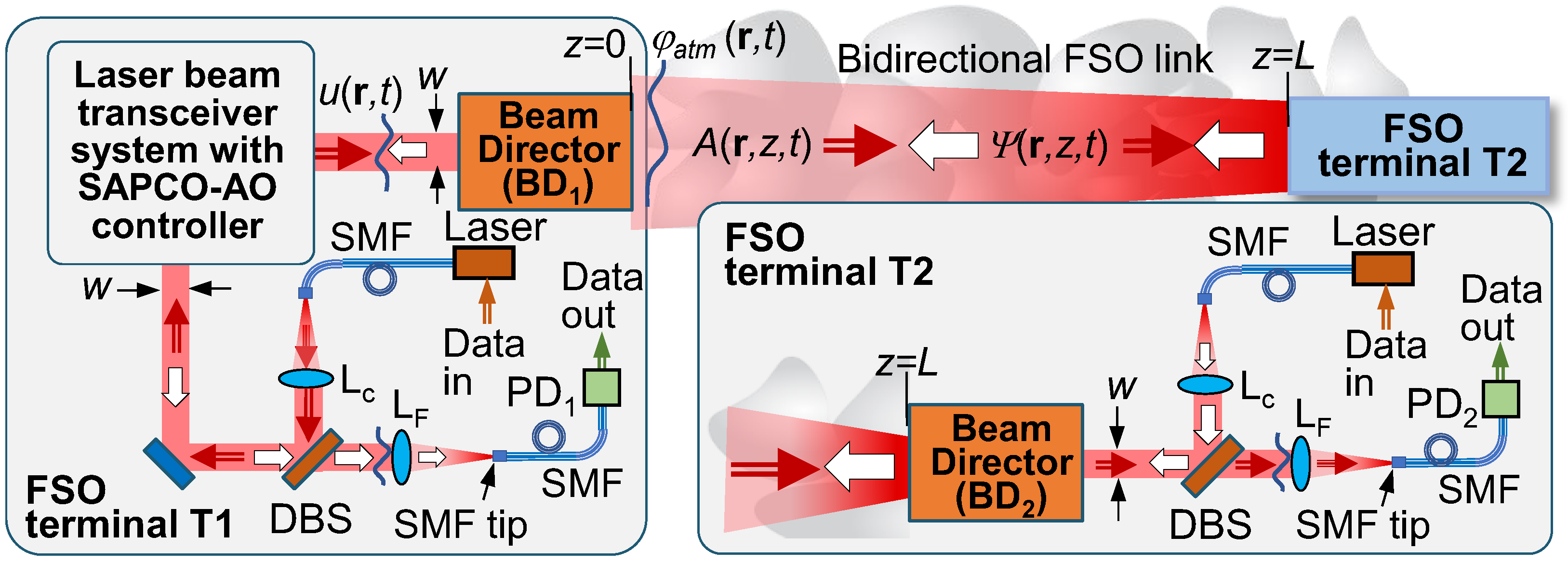
Figure 1 provides a notional schematic for a generic DE-LBP system architecture considered here. Wavefront control in this system is based on closed-loop instantaneous sensing and mitigation (pre-compensation) of atmospheric turbulence-induced phase aberrations by utilizing a single wavefront corrector – deformable mirror (DM). Note that the acronym DM is commonly applied independent of wavefront corrector type e.g., continuous surface or segmented type mirrors [10,11], or liquid crystal (LC)-based phase spatial light modulators (SLM) [12,13]. To simplify analysis and primarily focus on issues essential for IPR-based wavefront sensing and control we intentionally consider here only an idealized model for a segmented-type wavefront corrector that is comprised of a densely packed array of N_DM =n_DM x n_DM square mirrors (subapertures) providing independent control of subaperture-averaged (piston) phases. This wavefront corrector is referred to here as piston DM. The insert in Figure 1 illustrates a piston DM of with N_DM = 100 (n_DM=10) subapertures.

In practical A-AO systems the turbulence-induced tip and tilt (tip/tilt) phase aberration components are commonly pre-compensated using a special wavefront corrector, commonly referred to as beam steering mirror (BSM), and the corresponding feedback control system (not shown in Figure 1). For simplicity, here we assume that the BSM-based control enables complete removal of tip/tilt aberrations from the entering WFS optical field as discussed in Part I (Section 4.3). In the efficiency analysis of the SAPCO-AO control we consider operational regimes with and without preliminary removal of tip/tilt aberrations.

In the A-AO system in Figure 1, the BSM and DM are located inside the optical train shared by both the transmitted (outgoing) laser beam and received laser beacon (reference) wave – a typical arrangement for A-AO systems based on monostatic beam directors with phase conjugation (PC) – type control [9,14]. In these AO system types the pupil plane of the BD transceiver telescope is reimaged (with corresponding demagnification) to the BSM, DM, and WFS input plane (WFS aperture diaphragm). The reimaging optics (not shown in Figure 1) provides matching of the corresponding aperture sizes. Note that prior to entering the WFS the received reference (beacon) wave is reflected from the BSM and DM in the order illustrated in Figure 1.

The wavefront phase ${\phi }_{WFS}(M_{WFS}r,t)$ of the received optical field at the SAPCO WFS input plane can be represented in the form ${\phi }_{WFS}(M_{WFS}r,t)={\phi }_{atm}(r,t)+u_{DM}(M_{DM}r,t)+u_{BSM}(M_{BSM}r,t)$, where ${\phi }_{atm}(r,t)$ is the turbulence-induced phase aberration at the BD pupil plane, and $u_{DM}(M_{DM}r,t)$ and $u_{BSM}(M_{BSM}r,t)$ are controllable wavefront phase distributions introduced by the DM and BSM respectively. The demagnification factors M_DM, M_BSM and M_WFS in this expression describe rescaling of the BD aperture of size D to, correspondingly, the DM, BSM and WFS aperture sizes. In the M&S optical field demagnification can be accounted for by simple reassignment of the corresponding numerical grid pixel size. To simplify notation, we assume M_BSM = M_DM = M_WFS =1. In this case the received optical wave phase at the WFS input plane can be represented in the following simple form:

$${\phi }_{WFS}(r,t)={\phi }_{atm}(r,t)+u(r,t)$$

(1)

where $u(r,t)=u_{DM}(r,t)+u_{BSM}(r,t)$ is the controllable phase introduced into the transmitted beam and received (beacon) wave by the DM and BMS.

Similar as in Part I (Ref. [1]), in the M&S we consider a SAPCO WFS with square aperture of size D_WFS =D/M_D =3.55 mm, where M_D = 84.4 is the overall demagnification factor corresponding to reimaging of the BD aperture of size D =30 cm into the WFS aperture diaphragm. The parameters specified in M&S for D_WFS and D were chosen to correspondingly match the dimension of a commercially available CCD camera and a BD transceiver telescope aperture size typical for DE-LBP and remote laser power beaming applications. In analysis of the SAPCO-AO based FSO communication link in Section 4, we also considered laser transceivers with a BD aperture of size D =15 cm. In order to keep the parameter D_WFS unchanged, the demagnification factor M_D was reduced by two fold. The SAPCO WFS parameters used in numerical simulations, including phase mask characteristics, distances between WFS optical elements and the phase retrieval computational grid resolution (grid size N_PR), are identical as in Part I (see Section 3 and Section 4 in Ref. [1]).

In analysis of DE-LBP systems with SAPCO-AO control it is assumed that the reference optical wave is originated from a coherent monochromatic light source (laser beacon) located at the target aimpoint and that the beacon beam size d_b does not exceed the diffraction-limited size $d_{dif}\simeq d_{Airy}$(unresolved beacon) for the transmitter aperture of diameter D: $d_b\le d_{dif}=d_{Airy}$. Here $d_{Airy}=2.44\lambda L/D$ is the Airy disk diameter, λ is laser beacon wavelength, and L is distance from the BD transceiver telescope pupil plane to the target. The beacon beam is commonly generated in the DE-LBP systems using a supplementary illuminator laser system (not shown in Figure 1) that operates at a wavelength slightly different from the projected laser beam wavelength, thus enabling separation of the transmitted (outgoing) and received laser beacon optical waves inside the DE-LBP system optical train with a dichroic beam splitter (DBS), as illustrated in Figure 1. In M&S this difference in wavelengths was considered small and was neglected.

2.2. SAPCO-AO Feedback Control System

In the DE-LBP system schematic in Figure 1, the control voltages (controls) {a_j (t_n)} (j=1, …, N_DM) applied to DM actuators are sequentially updated at timesteps {t_n}, where t_n =nτ_AO and n=0,1, …, is number of sequential updates of the controls. It is expected that the duration τ_AO between control updates at each AO control cycle is considerably shorter than the characteristic correlation time τ_atm of atmospheric turbulence-induced phase aberrations (τ_AO << τ_atm). The correlation time τ_atm, also referred to as the atmospheric turbulence “frozen” time, depends on such factors as atmospheric turbulence strength, laser beam propagation geometry, cross-wing speed, and target velocity. For laser beam projection onto a stationary target τ_atm typically ranges from one to approximately one to ten milliseconds [15,16].

In the simplified piston DM model used in the numerical simulations, the phase modulation $u_{DM}(r,t)$ was considered as a static (time independent) function during each n-th AO control cycle (between the n-th and n+1-st updates of DM controls):

$$u_{DM}(r,t)=u_{DM}(r,t_n)={\displaystyle \sum _{j=1}^{N_{DM}}{v}_j(t_n)S_j(r)},(t_n\le t<t_{n+1}=t_n+{\tau }_{AO}).$$

(2)

Here $\{v_j(t_n)\}=\{c_j{a}_j(t_n)\}$ are phase modulation amplitudes resulting from the applied controls $\{a_j(t_n)\}$, $\left\{c_j\right\}$ are DM actuator sensitivity coefficients, and $\{S_j(r)\}$ are the DM response functions. For simplicity we further assume the piston DM model with identical actuator sensitivity coefficients $\left\{c_j\right\}=1$ and stepwise response functions $\{S_j(r)\}$ equal to one inside and zero otherwise of the corresponding DM subapertures of area s_sub. It was also assumed that the actuator response time τ_DM is distinctly smaller than τ_AO and, for this reason, was not accounted for in Eq. (2). However, in practical AO systems the response time τ_DM could be an important factor defining and/or limiting the AO control cycle duration τ_AO and, hence, the frequency bandwidth f_AO of the closed-loop control system. As a point of reference for piston-type (e.g., push-pool piezo, or dual-frequency LC cell-based) actuator response time estimation we consider ${\tau }_{DM}$=50 μs, which corresponds to the open-loop frequency bandwidth f_DM =20 kHz [10]. Note that piston phase control in coherent (phased) fiber array type BD systems can be performed with up to and above GHz-rate [17].

In the numerical simulations, performance of the DE-LBP system with a SAPCO-AO controller utilizing the piston DM was compared with the corresponding performance of a hypothetical (ideal) phase-conjugate (PC) AO system having infinitely high resolution in wavefront sensing and control, referred to here as the “ideal” phase-conjugate (IPC) AO system. The IPC phase pre-compensation can be represented in the form [9,14]:

$$u(r,t)=-{\phi }_{atm}(r,t)$$

(3)

where both the outgoing beam phase $u(r,t)$ and turbulence-induced aberration of the beacon beam ${\phi }_{atm}(r,t)$ are defined inside the BD transceiver aperture.

In the case of the SAPCO-AO control system considered here, the PC-type wavefront phase aberration pre-compensation algorithm can be described by the following iterative procedure for the control signal update:

$$a_j(t_{n+1})=a_j(t_n)-{\tilde{\phi }}_j(t_n),j=1,\dots ,N_{DM},t_n=n{\tau }_{AO},(n=0,1,\dots ),$$

(4)

where {${\tilde{\phi }}_j(t_n)$} are estimations of piston phases of the optical field entering the WFS computed during the n-th control cycle. Note that diacritic tilde symbol is used here and underneath to distinguish optical field characteristics obtained based on phase retrieval computations.

The piston phase estimations in Eq. (4) can be defined by the following expressions:

$${\tilde{\phi }}_j(t_n)=s_{sub}^{-1}{\displaystyle \int {\tilde{\phi }}_{WFS}(r,t_n)S_j(r)d^2}r,j=1,\dots ,N_{DM},t_n=n{\tau }_{AO},$$

(5)

where the function ${\tilde{\phi }}_{WFS}(r,t_n)$ represents estimation of the “true” residual (uncompensated) phase ${\phi }_{WFS}(r,t)$ [Eq. (1)] at the SAPCO sensor input plane during the n-th control cycle. The function ${\tilde{\phi }}_{WFS}(r,t_n)$ in Eq (5) is obtained in course of phase retrieval computations completed at time ${t^{\prime }}_n=t_{n+1}-{\tau }_{c-c}$ prior to the next update of controls. The time ${\tau }_{c-c}$ accounts for computation of the controls $\{a_j(t_{n+1})\}$ and their transfer to the DM actuators. Per benchmarking results conducted for n_DM =32 this time (on the order of ${\tau }_{c-c}\simeq$5 μs) represents a small fraction of the AO cycle duration τ_AO and for this reason was neglected in numerical simulations presented here. Note that since τ_AO << τ_atm, the “true” phase aberration ${\phi }_{WFS}(r,t)$ does not noticeably change between sequential update of controls and, hence, can be considered as static (“frozen”): ${\phi }_{WFS}(r,t)={\phi }_{WFS}(r,t_n)$.

Definition of piston phase estimations {${\tilde{\phi }}_j(t_n)$} in Eq. (4) through the retrieved phase ${\tilde{\phi }}_{WFS}(r,t_n)$ averaging over DM subaperture areas, as described by Eq. (5), may not be the best possible option. Under strong intensity scintillation conditions, the turbulence-induced phase aberration and, hence, the retrieved phase ${\tilde{\phi }}_{WFS}(r,t_n)$ may contain a considerable number of topological singularities (branch points and 2π phase cuts). Some of these phase singularities can be collocated with the DM subapertures resulting in ambiguity piston phase estimation based on Eq (5), unless the function ${\tilde{\phi }}_{WFS}(r,{t^{\prime }}_n)$ is preliminarily unwrapped [18]. However, phase unwrapping may be a challenging computational task especially with presence of noise resulting from phase retrieval calculations and rapid growth in the number of phase singularities with turbulence strength increasing [19]. In addition, phase unwrapping requires additional computational time leading to the need for additional τ_AO increase and corresponding decline in the AO control operational frequency bandwidth.

The ambiguity issue in piston phase estimations can be addressed by utilizing the following expression for computation of piston phases in the control algorithm (4) which is insensitive to the presence of phase singularities:

$${\tilde{\phi }}_j(t_n)=\arg {\displaystyle \int {\tilde{\Psi }}_{WFS}(r,t_n)S_j(r)d^2}r/{\displaystyle \int |{\tilde{\Psi }}_{WFS}(r,t_n)|S_j(r)d^2}r,$$

(6)

where ${\tilde{\Psi }}_{WFS}(r,t_n)={\tilde{I}}_{WFS}^{1/2}(r,t_n)\exp [i{\tilde{\phi }}_{WFS}(r,t_n)]$ and ${\tilde{I}}_{WFS}(r,t_n)$ correspondingly are the estimations of the received optical field complex amplitude and intensity at the SAPCO sensor input plane. These estimations can be obtained using the Fienup hybrid-input-output (HIO) complex field retrieval algorithm described in Part I (Ref [1]). A similar approach for computation of piston phases was proposed in Ref [20].

As numerical simulations show (see Section 2.5) utilization of PC-type control algorithm (4) with computation of the piston phase estimations based on Eq. (6) results in faster AO control process convergence, which is especially noticeable under strong scintillation conditions. For simplicity we further refer to the control algorithm Eq. (4) without specifying the exact formula [either Eq. (5), or Eq. (6)] used for piston phase computation, unless this difference is an important issue to be addressed. We also solely use the term “phase retrieval” even in conjunction with the computation of piston phase estimations [Eq. (5) or Eq. (6)] based on the HIO complex field retrieval algorithm.

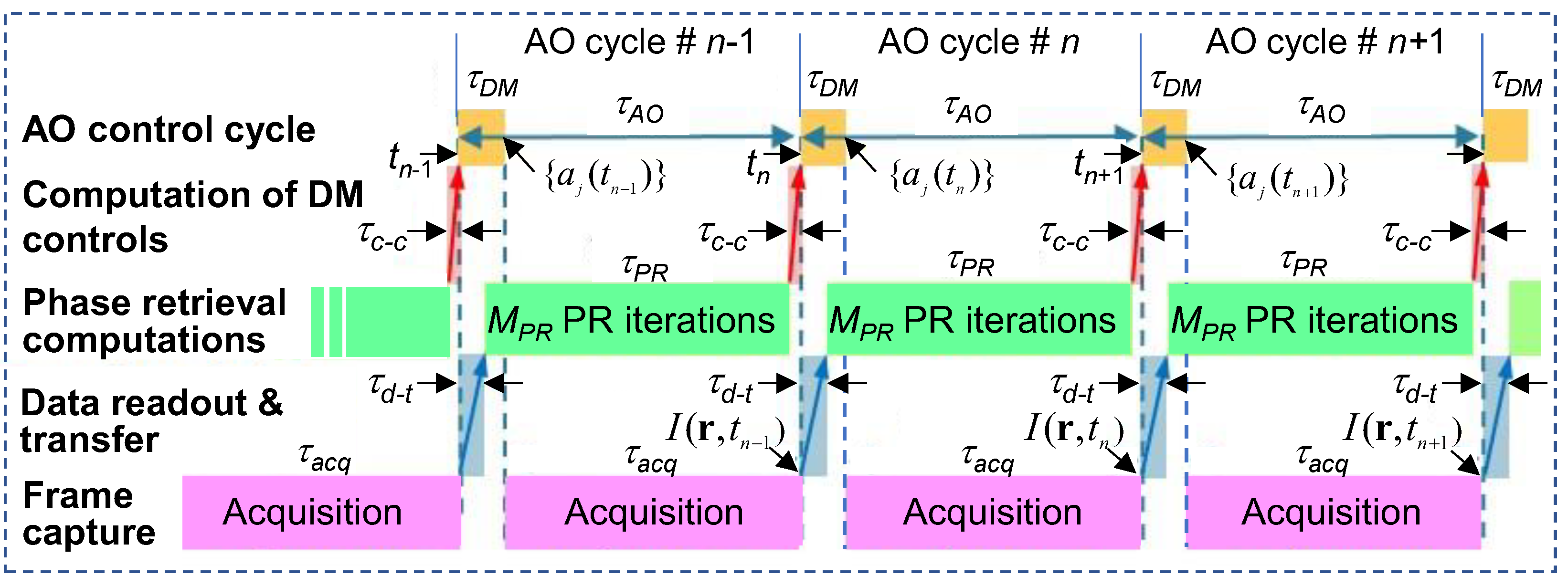
To conclude analysis of the SAPCO-AO control system model, consider the time diagram shown in Figure 2, that illustrates three sequential AO (DM controls update) cycles. Here the controls $\{a_j(t_{n+1})\}$ applied to the DM actuators at timestep t_n+1 are computed using Eq. (4). These controls depend on the estimation of residual phase ${\tilde{\phi }}_{WFS}(r,t_n)$ [or complex amplitude ${\tilde{\Psi }}_{WFS}(r,t_n)$] obtained during the preceding (n-th) control cycle. In its turn the function ${\tilde{\phi }}_{WFS}(r,t_n)$[or ${\tilde{\Psi }}_{WFS}(r,t_n)$] is computed during M_PR iterations of the HIO phase retrieval algorithm (HIO iterations). These HIO iterations are based on processing of the output intensity distribution $I_{out}(r,t_{n-1})$ of the SAPCO WFS which is acquired by the photo-array during the preceding (n-1)-st AO control cycle.

As the time diagram in Figure 2 shows, the intensity acquisition process starts at the timestep t_n-1 delayed by the DM actuator response time ${\tau }_{DM}$, and continues until the next (n-th) DM control update. This enables maximization of photo-array integration time ${\tau }_{acq}={\tau }_{AO}-{\tau }_{DM}$ during the AO control cycle and, therefore, the SNR improvement.

Intensity data readout and transfer to the phase retrieval processor are synchronized with control signal update at the n-th AO control cycle and occur during the time interval ${\tau }_{d-t}$, as shown in Figure 2. To increase the time ${\tau }_{PR}$ available for phase retrieval computation, the HIO iterations start after the completion of data readout and transfer, that is with the delay by ${\tau }_{d-t}$. For ${\tau }_{d-t}$ estimation assume that the intensity $I_{out}(r,t_{n-1})$ is acquired by a photo-array having 256 x256 pixels with 12-bit data resolution. With a commercial area-scan photo-array (e.g., from 1st Vision) and fast interface [e.g., CoaXPress, (Ref [21]), or Camera Link (Ref [22])] providing up to a 50Gbit/s data transmission rate, data readout and transfer would take approximately ${\tau }_{d-t}\simeq$30 μsec, or even less.

The major parameter defining the SAPCO-AO control cycle duration τ_AO is the time ${\tau }_{PR}=M_{PR}{\tau }_{it}$ required for phase retrieval (PR) computations. This time depends on the pre-selected number of PR iterations M_PR conducted between subsequent DM control updates and the computational time τ_it needed to perform a single PR iteration. Parameter M_PR increase leads to a more accurate estimation of the residual phase aberration at the WFS input plane and is therefore desired, but on the other hand this also results in an undesirable increase in control cycle duration τ_AO.

For a reasonably realistic estimation of the time scales ${\tau }_{PR}$ and τ_AO , consider results of PR iteration time ${\tau }_{it}$ benchmarking conducted for the SAPCO WFS configuration using a commercial gaming computer with a single GPU (see Section 3.2 in Part I, Ref. [1]). Phase retrieval computations performed using a numerical grid with resolution N_PR =256 (256x256 pixels) resulted in τ_it =133 μs. By accounting for the additional time required for data readout and transfer (${\tau }_{d-t}\simeq$30 μs) and controls computation (${\tau }_{c-c}\simeq$5 μs), for the shortest AO cycle with M_PR=1 we obtain ${\tau }_{AO}\simeq$ 170 μs. This suggests that the expected AO cycle duration ${\tau }_{AO}$ considerably exceeds the characteristic times ${\tau }_{DM}$,${\tau }_{d-t}$ and ${\tau }_{c-c}$, which for this reason were not accounted for in the described SAPCO-AO numerical model and M&S discussed below.

In principle, the phase retrieval iteration time τ_it and, hence τ_PR can be significantly (up to several fold) decreased with transitioning to specialized (e.g. FPGA-based) signal processing hardware. Nevertheless, this may not result in the intended increase in the closed-loop AO control system bandwidth frequency f_AO without corresponding decreases in the DM actuator response (${\tau }_{DM}$) and data readout / transfer (${\tau }_{d-t}$) times. Additionally, for a low power beacon the major limiting factor in τ_AO decrease could be insufficiently long (for achieving acceptable SNR) acquisition time τ_acq of the WFS output intensity $I_{out}(r,t_n)$. The issues mentioned above are common for all A-AO system types utilizing WFSs and DMs, not just for the SAPCO-AO architecture considered here.

2.3. Mathematical and Numerical Models: Modeling and Simulation Setting

In this section we continue analysis of the mathematical and numerical models for the generic DE-LBP system based on SAPCO-AO control shown in Figure 1. Atmospheric propagation of the monochromatic transmitted and received (beacon) optical waves can be described by the following system of parabolic equations for the complex amplitudes of the outgoing (projected)$A(r,z,t)$ and backpropagating (beacon) $\Psi (r,z,t)$ optical waves [14,23,24,25]:

$$2ik{\displaystyle \frac{\partial A(r,z,t)}{\partial z}}={\nabla }_{\perp }^{2}A(r,z,t)+2k^2{n}_1(r,z,t)A(r,z,t),0\le z\le L,$$

(7)

$$-2ik{\displaystyle \frac{\partial \Psi (r,z,t)}{\partial z}}={\nabla }_{\perp }^2\Psi (r,z,t)+2k^2{n}_1(r,z,t)\Psi (r,z,t),0\le z\le L,$$

(8)

where ${\nabla }_{\perp }^2={\partial }^2/\partial x^2+{\partial }^2/\partial y^2$ is the Laplacian operator, $n_1(r,z,t)$ is a random field realization describing the atmospheric turbulence-induced refractive index perturbations from the undisturbed value n₀, and $k=2\pi n_0/\lambda$. The refractive index perturbations are assumed as statistically homogeneous, isotropic, and obey the Kolmogorov power spectrum law [23,25]. An identical wavelength (λ=1064 nm) is considered for both the outgoing and beacon waves in Eq. (7) and Eq. (8). This wavelength (λ=1064 nm), most common for DE-LBP applications, was also considered in analysis and M&S of remote laser power beaming (Section 3) and FSO laser communications (Section 4) even though latter systems are typically based on laser sources having other wavelengths (e.g., λ=1550 nm is more common for FSO communication links [6]). The use of an identical wavelength throughout this paper was selected for easier and more consistent comparison of SAPCO-AO control performance across the applications considered. The presented results can easily be adapted for each specific application wavelength.

Similar as in Part I (Section 2.2), the atmospheric turbulence impact on AO system performance is characterized here by the ratio D/r₀ of the BD aperture of size D to the Fried parameter r₀ (the measure of the phase aberration correlation length at the propagation path end), and the Rytov variance ${\sigma }_R^2$ describing the strength of intensity scintillations at the BD pupil plane. Both the D/r₀ and ${\sigma }_R^2$ depend on the refractive index structure parameter $C_n^2$, propagation distance L, and wavelength λ (see Section 2.2, Part I) [1,23,24].

The complex amplitude $A(r,z=0,t)\equiv A(r,0,t)$ of the projected laser beam at the BD pupil plane (z =0) defines the boundary condition for Eq. (7):

$$A(r,0,t)=A_0(r)\exp [iu(r,t)]$$

(9)

where $A_0(r)=I_0^{1/2}(r)$ and $I_0(r)$ correspondingly are the transmitted beam magnitude and intensity distributions. For the flat-top transmitted beam considered here and in Section 3 $I_0(r)=I_0=const$ inside the BD aperture and zero otherwise. In the M&S the flat-top beam was approximated by a super-gaussian function of power 8 and width D.

The controllable phase $u(r,t)$ in Eq. (9) is described by the following expression:

$$u(r,t)=u_{DM}(r,t_n)+u_{BSM}(r,t)={\displaystyle \sum _{j=1}^{N_{DM}}{a}_j(t_n)S_j(r)}+u_{BSM}(r,t),t_n\le t<t_{n+1},$$

(10)

where the controls $\{a_j(t_n)\}$ are computed using the PC-type algorithm defined by Eq. (4). In the M&S the phase modulation component $u_{BSM}(r,t)$ in Eq. (10) was set either to zero for the operational regime without a BSM-based tip/tilt control, or $u_{BSM}(r,t)=-{\phi }_{atm}^{t-t}(r,t)$ when the tip/tilt phase aberration component ${\phi }_{atm}^{t-t}(r,t)$ of the input field wavefront phase ${\phi }_{atm}(r,t)$ was completely removed prior to control update at each AO control cycle using a hypothetical (ideal) tip/tilt control system.

In numerical simulations the tip/tilt aberration component ${\phi }_{atm}^{t-t}(r,t)$ was defined through the wavefront slope vector $\theta (t)=\{{\theta }_x(t),{\theta }_y(t)\}$ corresponding to the input field complex amplitude $\Psi (r,0,t)$: ${\phi }_{atm}^{t-t}(r,t)={\theta }_x(t)x+{\theta }_y(t)y$. In its turn the slope vector was represented in the form $\theta (t)=r_c(t)/F$, where $r_c(t)=\{x_c(t),y_c(t)\}$ is the vector describing centroid displacement of the intensity distribution in the focal plane of a virtual ideal (infinite size, thin, parabolic) lens with a focal distance F that can be arbitrary selected in simulations (”virtual” lens technique for wavefront slope computation [26]). A similar approach is utilized for computation of wavefront tip/tilts within the lenslet subapertures of a Shack-Hartmann WFS [27].

Consider now Eq. (8) describing laser beacon beam propagation from the target (z=L) to the BD transceiver telescope plane (z=0). The boundary condition for this equation is defined by the complex amplitude

$$\Psi (r,z=0,L,t)\equiv \Psi (r,L,t)=I_b^{1/2}(r)\exp [i{\phi }_b(r,t)]$$

(11)

Where $I_b(r)$ and ${\phi }_b(r,t)$ are the beacon beam intensity and phase distributions.

In M&S of the DE-LBP AO system we considered a collimated [${\phi }_b(r,t)$=const] super-gaussian beacon beam of width d_b = 0.25d_Airy located a distance L= 5 km from the BD transceiver telescope. In the absence of turbulence, the beacon beam footprint size at the transceiver plane (z=0) was approximately two-fold larger than the BD aperture size (D = 30 cm) and two-fold smaller than the physical size of the simulation area corresponding to a 120-cm square with approximately ${\Delta }_{pixel}$=2.34 mm pixel size.

The propagation Eq. (8) with the boundary condition (11) defines the complex amplitude $\Psi (r,0,t)$ of the entering BD received wave, which can be represented in the following form:$\Psi (r,0,t)=I_{in}^{1/2}(r)\exp [i{\phi }_{in}(r,t)],$ where $I_{in}(r,t)=|\Psi (r,0,t){|}^2$ and ${\phi }_{in}(r,t)=\arg [\Psi (r,0,t)]$ are the input wave intensity and phase distributions. In its turn the input field phase ${\phi }_{in}(r,t)$ includes an independent on turbulence (static) phase component ${\phi }_0(r)$ that is defined by beacon beam propagation geometry and the turbulence-induced phase aberration component ${\phi }_{atm}(r,t)$, that is ${\phi }_{in}(r,t)={\phi }_0(r)+{\phi }_{atm}(r,t)$. In the DE-LBP model considered here the static phase represents a parabolic phase corresponding a spherical wave originated at the laser beacon location. It is assumed that this phase component is compensated within the transceiver telescope optical assembly, so the complex amplitude of the optical field entering WFS can be represented in the form:

$${\Psi }_{WFS}(r,t)=I_{WFS}^{1/2}(r,t)\exp [i{\phi }_{WFS}(r,t)]$$

(12)

where $I_{WFS}(r,t)=W_{WFS}(r)I_{in}(r,t)$ is intensity distribution inside the WFS aperture diaphragm described by the window function $W_{WFS}(r)$ (step-wise function within a square of size D_WFS), and ${\phi }_{WFS}(r,t)={\phi }_{atm}(r,t)+u(r,t)$. Here we accounted for the controllable phase modulation [Eq (10)] introduced by the DM and BSM inside the BD optical train.

Mathematical model describing transformation of the complex amplitude ${\Psi }_{WFS}(r,t)$ [Eq. (12)] inside the SAPCO WFS resulting in the output intensity distribution $I_{out}(r,t_n)$ captured by the sensor photo-array during n-th AO control cycle is presented in Part I (see Section 2.3 in Ref. [1]) and for this reason is omitted here. In summary, the mathematical model of the DE-LBP system with SAPCO-AO control used in numerical simulations includes:

(a)

the beacon beam propagation equation [Eq. (8)] with the boundary condition [Eq. (11)];

(b)

expressions defining the controllable phase $u(r,t)$ [Eq. (9)] and the complex amplitude of the entering WFS field with complex amplitude ${\Psi }_{WFS}(r,t)$ [Eq. (12)];

(c)

wavefront phase aberration pre-compensation algorithm describing sequential updates of controls $\{a_j(t_n)\}$ [Eq. (4)] with options [Eq. (5) or Eq. (6)] for computation of piston phase estimation $\{{\tilde{\phi }}_j(t_n)\}$,

(d)

the HIO phase retrieval (PR) algorithm applied for the SAPCO WFS optical configuration model described in Part I (see sections 2.3-2.6 in Ref. [1]) providing the estimation ${\tilde{\Psi }}_{WFS}(r,t_n)$ of the entering WFS complex amplitude in a set of M_PR phase retrieval (PR) iterations conducted for each n-th AO control cycle, which is needed for computation of piston phase estimations in the control algorithm, and

(e)

propagation equation [Eq. (7)] for the projected laser beam with the boundary conditions [Eq. (9)] enabling computation of the target-plane intensity distribution $I_T(r,t)=|A(r,z=L,t){|}^2$ and efficiency assessment of the SAPCO-AO control via computation of laser beam projection performance metrics.

In M&S the numerical integration of Eq. (7) and Eq. (8) with boundary conditions defined by Eq. (9) and Eq. (11) was performed on a computational grid with resolution N_atm =512 (512x512 pixels) using the wave-optics (split-step operator-based) technique (Ref [24,28]). The central part of this grid with resolution N_PR = N_atm /2 and scaled by factor M_D = 84.4 pixel size, was used for HIO phase retrieval computations. The area of the SAPCO WFS square aperture diaphragm of size D_WFS was represented on the grid with resolution N_WFS =128.

As in Part I (Ref. [1]) turbulence-induced refractive index inhomogeneities along the propagation path for both the beacon and transmitted laser beams were represented by a set of N_φ =20 equally spaced 2D random thin phase screens corresponding to the Kolmogorov turbulence power spectrum. The combinations of N_φ mutually uncorrelated phase screens are referred to here as turbulence realizations.

To simulate cross-wind impact on SAPCO-AO control system performance, numerical integration of Eq. (7) and Eq. (8) was conducted in a sequence of timesteps. For convenience, the time interval Δt between sequential timesteps was set equal to the shortest AO cycle duration τ_AO corresponding to single PR iteration (M_PR= 1): Δt = τ_it =133 μs. The overall number of time steps was set to be sufficiently large to ensure SAPCO-AO control process convergence, or (in the absence of convergence) to reveal general trends in the cross-wind impact on DE-LBP system performance.

For M&S of cross-wind-induced effects we assumed validity of Taylor’s “frozen” turbulence hypothesis [15,29]. Correspondingly, phase screens were shifted along the ox axis (wind speed direction) at each timestep by the number of grid pixels dependent on the cross-wind velocity v₀. Note that numerical analysis of DE-LBP system performance in the presence of strong cross-wind (and/or in operation with a fast-moving target) may require phase screen shifts over number of pixels exceeding the computational grid size. To preserve continuity in phase aberrations for these operational scenarios, turbulence phase screens were generated inside a 4x-elongated (along the ox-axis) computational area. These elongated phase screens, also referred to as “infinitely-long” turbulent phase screens (Ref. [30]), were continuously regenerated with sequential phase screen shifts. The mathematical and numerical models presented in this section describing the DE-LBP system with SAPCO-AO controller are equally applicable (and were further used) for analysis of AO control in remote power beaming and FSO communication systems (with a few minor adjustments described in corresponding sections of this paper).

2.4. Performance Metrics

Performance of the SAPCO-AO based DE-LBS system was evaluated using the following measures (metrics):

(a)

Phase error metric ${\epsilon }_{\delta }^{AO}(t)$ characterizing residual (uncompensated) phase aberration ${\phi }_{WFS}(r,t)={\phi }_{atm}(r,t)+u(r,t)$ within the WFS aperture diaphragm as described by the window function $W_{WFS}(r)$. The phase error metric computed during sequential updates of the DM controls was defined as:

$${\epsilon }_{\delta }^{AO}(t)=1-D_{WFS}^{-2}{\left|{\displaystyle \int W_{WFS}(r)\exp [i{\phi }_{WFS}(r,t)]d^{2}r}\right|}^2.$$

(13)

Similar to performance measures used for analysis of PR algorithms in Part I (see Section 2.7), the metric (13) is insensitive to modulo 2π phase jumps in the residual phase. The phase error metric values depend on the pre-selected set of SAPCO-AO control system parameters including resolution of the piston DM (n_DM), geometry and parameters of the SAPCO WFS, chosen number of HIO iterations M_PR, etc. It is also convenient to represent ${\epsilon }_{\delta }^{AO}(t)$ in Eq. (13) as function of either the number of sequential control signal updates [${\epsilon }_{\delta }^{AO}(n)$], or as a function of the normalized time ${\epsilon }_{\delta }^{AO}(t/{\tau }_{it})$ or ${\epsilon }_{\delta }^{AO}(t/{\tau }_{AO})$.

The metric (13) solely characterizes AO control system performance in mitigation of phase aberrations within the WFS aperture diaphragm, and only indirectly the overall DE-LBP system effectiveness in maximization of projected laser power density at the target plane. The latter characteristic is influenced by several additional factors, including the BD transceiver telescope and projected laser beam parameters (e.g., BD type, aperture size, beam intensity and phase distributions), propagation geometry (e.g., distance and elevation of the BD transceiver and target), and turbulence strength and distribution along the propagation path (turbulence profile). For this reason, the overall laser beam projection efficiency with SAPCO-AO control was evaluated in the M&S using the target-plane power-in-the-bucket (PIB) metric, that combines the impact of all the factors mentioned above.

(b)

The PIB metric $J_{PIB}(t)$ [or equivalently $J_{PIB}(n)$, or $J_{PIB}(t/{\tau }_{it})$, or $J_{PIB}(t/{\tau }_{AO})$] was defined in M&S as the projected laser beam power (normalized by the overall transmitted beam power P₀) inside the target-plane on-axis circle [bucket $b_T(r)$] of diameter $d_{PIB}=(2/3)d_{Airy}$:

$$J_{PIB}(t)=P_0^{-1}{\displaystyle \int b_T(r)I_T(r,t)]d^{2}r}$$

(14)

For comparison, we also computed the PIB metric values $J_{PIB}^{IPC}$ and $J_{PIB}^{IPC-DM}$ corresponding to the IPC control algorithm [Eq. (3)] utilizing either a hypothetical DM having “infinitely” high resolution (numerical grid resolution n_WFS=128 in the M&S setting used), or the PC-type control algorithm [similarly to Eq. (4)] for a system with a piston DM composed of N_DM =n_DM x n_DM actuators $(J_{PIB}^{IPC-DM})$. In the latter case the controls were defined as $\{a_j(t)\}=-\{{\phi }_j(t)\}$, where the piston phases $\{{\phi }_j(t)\}$ were computed using the following expression [analogous to Eq. (6)]: ${\phi }_j(t)=\arg {\displaystyle \int \Psi (r,0,t)S_j(r)d^2}r/{\displaystyle \int |\Psi (r,0,t)|S_j(r)d^2}r$ (j=1,…,N_DM). Metric $J_{PIB}^{IPC}$ characterizes the performance that can be theoretically achieved with an ideal PC-type control system under specified turbulence conditions. On the other hand, $J_{PIB}^{IPC-DM}$ represents a maximum PIB metric value achievable with a selected piston DM comprised of n_DM x n_DM actuators.

Both metrics ${\epsilon }_{\delta }^{AO}(t)$ and $J_{PIB}(t)$ depend on the specific turbulence realizations along the propagation path used in the M&S. For performance assessment in statistical terms the metrics ${\epsilon }_{\delta }^{AO}(t)$ and $J_{PIB}(t)$ were computed in a set of N_trial =100 adaptation (AO) trials. Each trial was composed of N_update sequential DM control updates, began with zero controls $\{a_j(t_0=0)\}=0$ and conducted using statistically independent atmospheric turbulence realization for each trial. The AO trials resulted in computation of N_trial dependences $\{{\epsilon }_{\delta }^{AO}(t)\}$ and $\{J_{PIB}(t)\}$ characterizing AO process time evolution for selected turbulence conditions, which were averaged over adaptation trial numbers. The obtained dependences $<{\epsilon }_{\delta }^{AO}(t){>}_{atm}$ and $<J_{PIB}(t){>}_{atm}$ referred to as atmospheric-averaged performance metric adaptation curves, were further used for both SAPCO-AO control efficiency assessment under specified turbulence conditions and for optimization of the control system parameters.

2.5. SAPCO-AO Control System Parameter Optimization

Performance analysis of the DE-LBP system in Figure 1 (as well as the remote power beaming and FSO communications systems in Section 3 and Section 4) requires initial setting of SAPCO-AO control system characteristics including:

• Selection of an initial estimation (defined by the superscript m=0) for the complex amplitude of the field entering the WFS ${\tilde{\Psi }}_{WFS}^{(m=0)}(r,t_n)=|{\tilde{\Psi }}_{WFS}^{(m=0)}(r,t_n)|\exp [i{\tilde{\phi }}_{WFS}^{(m=0)}(r,t_n)]$ to be used as an initial condition for M_PR HIO phase retrieval (PR) iterations conducted at each AO control update timestep {t_n} (n=0,1,…). The following two options, referred to here as “Reset” and “Preceding AO cycle,” were examined through M&S. In the first “Reset” case initial estimations for the magnitude $|{\tilde{\Psi }}_{WFS}^{(m=0)}(r,t_n)|$ were always (for all timesteps) set to a constant, while for the initial phase estimations ${\tilde{\phi }}_{WFS}^{(m=0)}(r,t_n)$ we used statistically independent (for each n) random 2D realizations of a delta-correlated field with zero mean and uniform probability distribution inside the interval [-π, π].
  In the “Preceding AO cycle” case, the complex amplitude ${\tilde{\Psi }}_{WFS}^{(m=M_{PR})}(r,t_{n-1})$ computed at the end of the preceding (n-1)-st AO control cycle (after completion of M_PR PR iterations) was used:${\tilde{\Psi }}_{WFS}^{(m=0)}(r,t_n)={\tilde{\Psi }}_{WFS}^{(m=M_{PR})}(r,t_{n-1})$. Both PR initial condition options are described in more detail in Part I (Section 2.6), Ref [1].
• Selection of either Eq. (7) or Eq. (8) for computation of piston phase estimation $\{{\tilde{\phi }}_j(t_n)\}$ in the control algorithm (6).
• Selection of how many PR iterations M_PR per AO control cycle should be performed to minimize the overall adaptation process convergence time τ_conv and hence increase the AO control system closed-loop frequency bandwidth f_AO =1/ τ_conv. The AO process convergence time τ_conv = M_conv τ_it is defined here through the overall number of PR iterations M_conv or the corresponding number N_conv = M_conv / M_PR of sequential control updates, which are required to achieve a pre-selected threshold value $J_{PIB}^{th}$ of the atmospheric-averaged PIB metric: $<J_{PIB}(m=M_{conv}){>}_{atm}\ge J_{PIB}^{th}$. In the M&S the threshold $J_{PIB}^{th}$ was set to 90% of the maximum atmospheric-averaged PIB metric value achieved during AO control trials composed of N_update =20 control updates: $J_{PIB}^{th}=0.9\underset{t}{\max }\left[<J_{PIB}(t){>}_{atm}\right]$, where $0\le t\le T_{trial}$ and T_trial = N_update τ_AO = N_update M_PR τ_it.

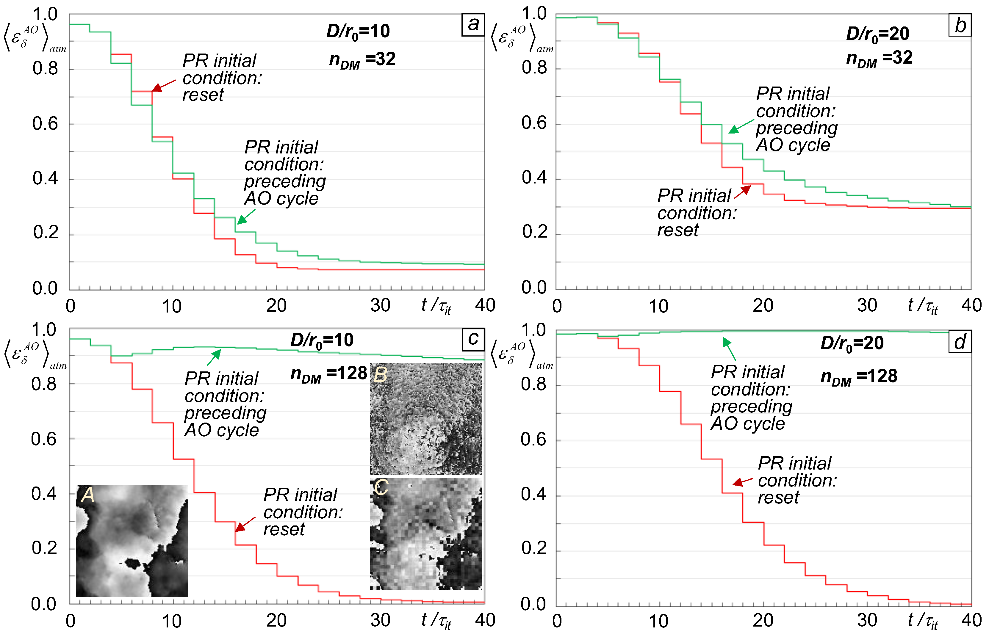
To choose between the “Reset” and “Preceding AO cycle” options consider the time-evolution dependencies $<{\epsilon }_{\delta }^{AO}(t/{\tau }_{it}){>}_{atm}$ shown in Figure 3 illustrating the dynamics of atmospheric-averaged phase error metric evolution during sequential control updates for both PR initial conditions. Notice the monotonic decrease (convergence) of the phase error metric $<{\epsilon }_{\delta }^{AO}(t/{\tau }_{it}){>}_{atm}$ independent of the pre-selected PR initial condition for the piston DM with n_DM =32. On the contrary, in the case of a higher resolution DM (n_DM =128), AO process convergence occurred only for the “Reset” PR initial condition as shown in Figure 3 (c, d). The “Reset” option also provides faster convergence and smaller residual phase error for all cases considered in Figure 3. For this reason, the “Reset” PR initial condition was used in all numerical simulations described below.

The reason why an intuitively preferable “Preceding AO cycle” PR initial condition option, which should take advantage of PR computations conducted at the preceding control cycle, resulted in less stable and slower AO process convergence can be explained by considering the characteristic spatial structure of the phase estimations $\{{\tilde{\phi }}_{WFS}^{(m=1)}(r,t_n)\}$ obtained after the few first PR iterations at each n-th control update cycle. These phase estimations are commonly characterized by the presence of strong digital noise that gradually decreases with increasing m (m=1,…, M_PR). With selection of the “Preceding AO cycle” option with a small PR parameter M_PR (e.g., M_PR =1 or M_PR =2 as in Figure 3) the digital noise in the phase estimations $\{{\tilde{\phi }}_{WFS}^{(m=M_{PR})}(r,t_n)\}$ obtained at the end of the PR iterations remains strong and, hence, negatively affects the controllable phase $u_{DM}(r,t_{n+1})$ for the following control cycle. This results in digital noise “propagation” through sequential AO control cycles potentially leading to slowing of the AO process convergence or even instability.

To illustrate, consider the grey-scale insert images in Figure 3 (c). The image “A” presents a characteristic example of initial phase aberration ${\phi }_{WFS}(r,t_0=0)$ at the WFS aperture diaphragm for D/r₀ =10 and $u(r,0)=0$. The corresponding phase estimation ${\tilde{\phi }}_{WFS}^{(m=2)}(r,t_1)$ obtained after two sequential PR iterations and shown in image “B” exhibits a clearly visible presence of digital noise. The impact of this noise is less obvious in the controllable phase $u(r,t_1)$ (image “C”) for DM with n_DM =32. The noise decrease in image “C” occurs due to averaging of the noisy phase estimation pattern ${\tilde{\phi }}_{WFS}^{(m=2)}(r,t_0)$ (image “B”) over the DM subaperture areas. This averaging takes place in computation of the piston phases [Eq. (5)] and the corresponding controllable phase $u_{DM}(r,t_1)$ [Eq. (4)].

The higher the DM resolution, the less efficient is the subaperture averaging-based digital noise suppression. With selection of the “Preceding AO cycle” option, small M_PR, and a high-resolution DM, the digital noise increases through consecutive AO cycles leading to possible AO control instability, as in the case shown in Figure 3 (c, d) for n_DM =128. On the other hand, the “Reset” option prevents such digital noise amplification through DM control updates and for this reason is preferable. As already mentioned, the digital noise component gradually decreases with M_PR increase and for this reason is desired. At the same time parameter M_PR increase for better digital noise suppression leads to an unwanted increase of the AO control cycle duration τ_AO.

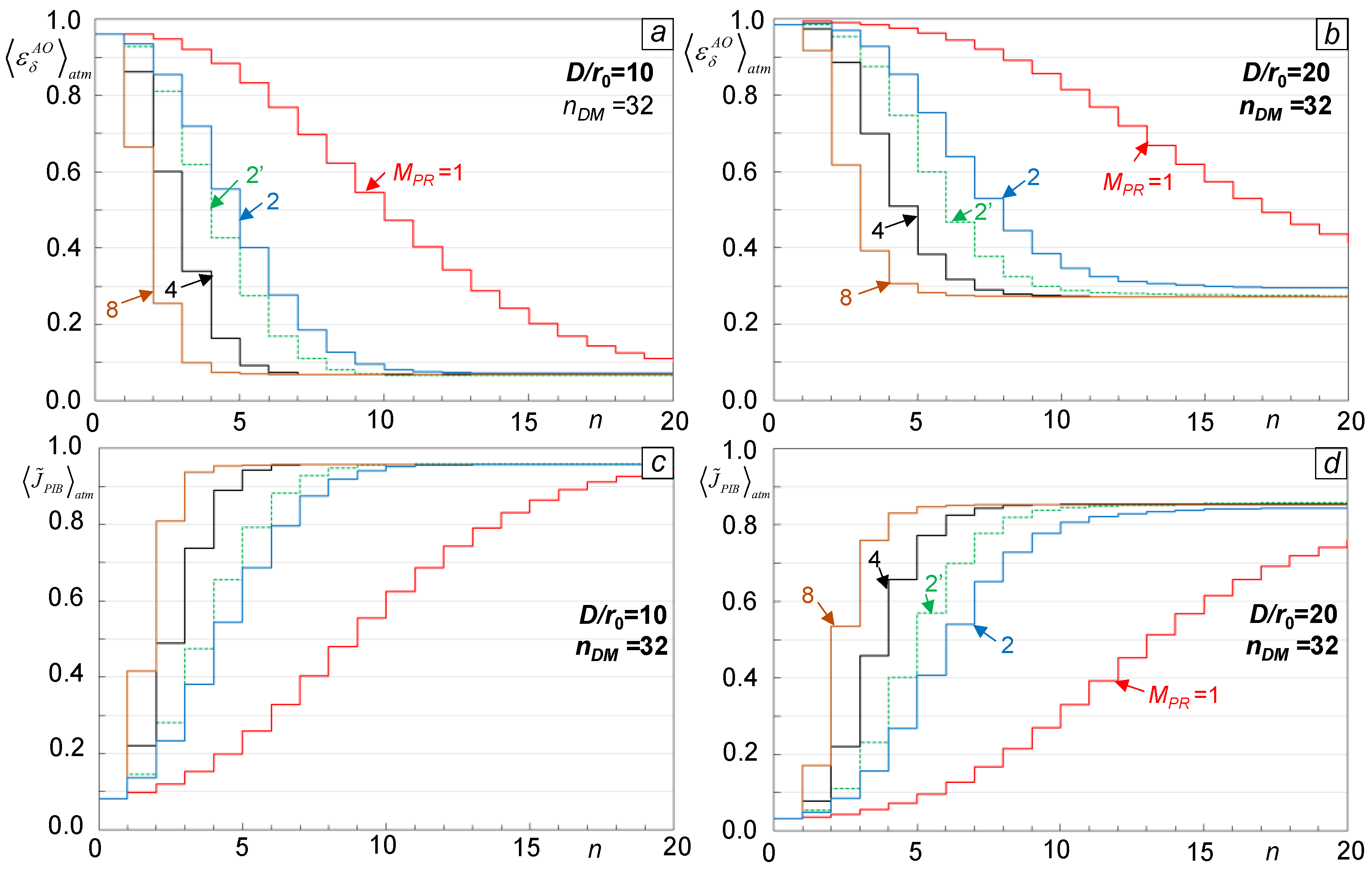
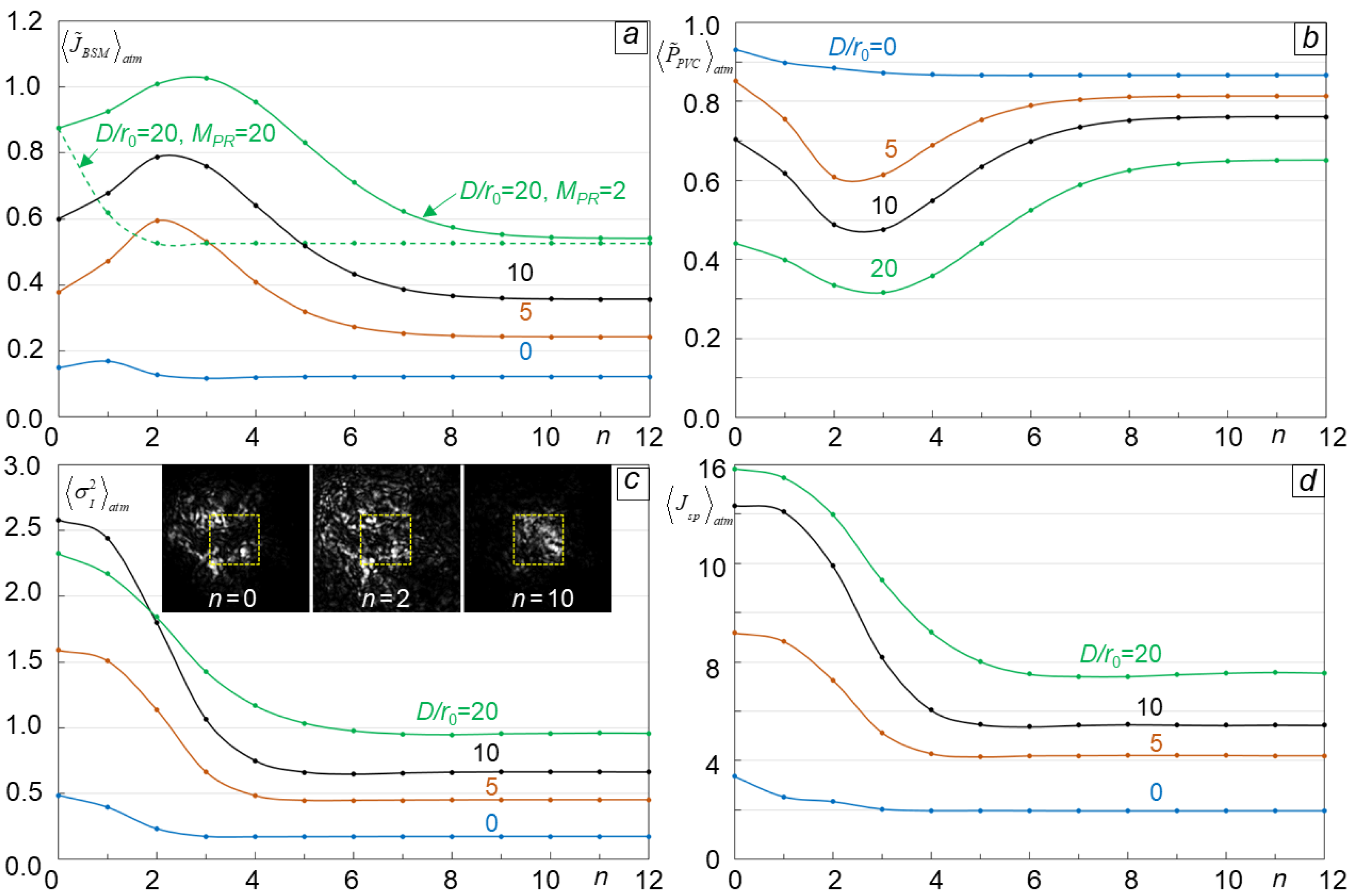
To investigate tradeoffs in parameter M_PR selection for the SAPCO-AO control system, consider dependencies of the atmospheric-averaged residual phase error $<{\epsilon }_{\delta }^{AO}(n){>}_{atm}$ shown in Figure 4 (a),(b) and the corresponding normalized PIB metric ${〈{\tilde{J}}_{PIB}(n)〉}_{atm}={〈J_{PIB}(n)〉}_{atm}/{〈J_{PIB}^{IPC}〉}_{atm}$ computed for $d_{PIB}=(2/3)d_{Airy}$ in Figure 4 (c), (d) on the consecutive control update number n, computed for different parameter M_PR values. As expected, the increase in the number of PR iterations per AO cycle (parameter M_PR increase), aiming to achieve better phase retrieval accuracy during each DM control cycle, resulted in a lesser number of control updates required for reaching stationary performance metric values (faster convergence in terms of the overall number of DM control updates).

As can be seen from the AO process convergence curves in Figure 4, utilization of a single PR iteration per control update (M_PR =1) leads to noticeably slower (compared with M_PR >1) convergence for all considered M&S cases, which can be explained by the negative impact of digital noise described above. Note that for M_PR > 1 and n_DM =32 the PIB metric values ${〈J_{PIB}(n=N_{update})〉}_{atm}$ achieved at the adaptation trial end (after N_update =20 control updates) are comparable with the corresponding values ${〈J_{PIB}^{IPC}〉}_{atm}$ for an “ideal” phase-conjugate (IPC) AO control system operating under identical turbulence conditions. The difference does not exceed 5% for D/r₀ = 10 and 15% for D/r₀ = 20.

The AO process convergence curves (solid lines in Figure 4) were computed using control algorithm (4) with piston phases defined by Eq. (5), that is through the retrieved phase estimation ${\tilde{\phi }}_{WFS}(r,t_n)$ averaging over the DM subaperture areas. For comparison, corresponding AO process convergence curves were also computed using Eq. (6) that defines piston phases via subaperture-averaging of the complex amplitude estimation ${\tilde{\Psi }}_{WFS}(r,t_n).$ These AO convergence curves are shown in Figure 4 (for only M_PR =2) by dashed lines. In all cases considered, piston phase computations based on Eq. (6) resulted in faster AO process convergence, which is more evident under stronger turbulence conditions. Based on these results and, since retrieval of the phase ${\tilde{\phi }}_{WFS}(r,t_n)$ and complex amplitude ${\tilde{\Psi }}_{WFS}(r,t_n)$ requires identical computational times, in all numerical simulations presented below we exclusively used Eq. (6) for piston phase computation.

To estimate the SAPCO-AO control process convergence time τ_conv and select the optimal number of PR iterations per control cycle (parameter M_PR), consider time dependencies (adaptation process convergence curves) of the normalized atmospheric-averaged PIB metric $<{\tilde{J}}_{PIB}(t/{\tau }_{it}){>}_{atm}=<J_{PIB}(t/{\tau }_{it}){>}_{atm}/<J_{PIB}^{IPC}{>}_{atm}$ presented in Figure 5. The simulations were performed for M&S parameters identical to those in Figure 4 (c, d) and with use of Eq. (6) for piston phase computation. For comparison, the dashed line in Figure 5 (marked as 2’’) illustrates AO process convergence for the case of tip/tilt aberration removal with M_PR =2.

The results presented in Figure 5 were utilized to estimate the adaptation process convergence time τ_conv and closed-loop frequency bandwidth f_AO =1/τ_conv. The threshold value $J_{PIB}^{th}$ used for τ_conv and f_AO estimations was set to 90% of the maximum (with respect to all examined M_PR values) atmospheric-averaged PIB metric value achieved at the end of the adaptation trials (at $t=T_{trial}=40{\tau }_{it}$).

Convergence time estimation results for several parameter M_PR values and turbulence strengths (for D/r₀ =10 and D/r₀ =20) are presented in Table 1. The tip/tilt removal operational regime with M_PR =2 is indicated by M_PR =2’’. As seen from Table 1, the fastest AO process convergence occurs with selection of two phase retrieval iterations (M_PR =2) between sequential control updates for both turbulence conditions examined. Tip/tilt aberration removal results in approximately a 1.2-fold faster convergence for D/r₀ =10 but does not make any difference under strong turbulence.

Using τ_it =133 μs as a point of reference (benchmarked value obtained using a commercial gaming PC in Ref. [1]) for the SAPCO-AO controller with selection of an optimal number of PR iterations per AO control cycle M_PR =2 we derive to the following estimtions: τ_conv ~ 1.6 ms for D/r₀ =10 and τ_conv ~ 1.8 ms for D/r₀ = 20. This corresponds to f_AO ~ 0.6 kHz for D/r₀ =10 and f_AO ~ 0.5 kHz for D/r₀ = 20. As already mentioned, the phase retrieval iteration time τ_it and, hence τ_AO and τ_conv can be significantly decreased by utilizing specialized (e.g., FPGA-based) signal processing hardware, which makes technically feasible (unless limited by the DM actuator response time) the development of A-AO systems capable of operation in strong scintillation conditions exceeding a 1.0 kHz closed-loop frequency bandwidth.

2.6. Laser Beam Projection with SAPCO-AO Control: Performance Assessment

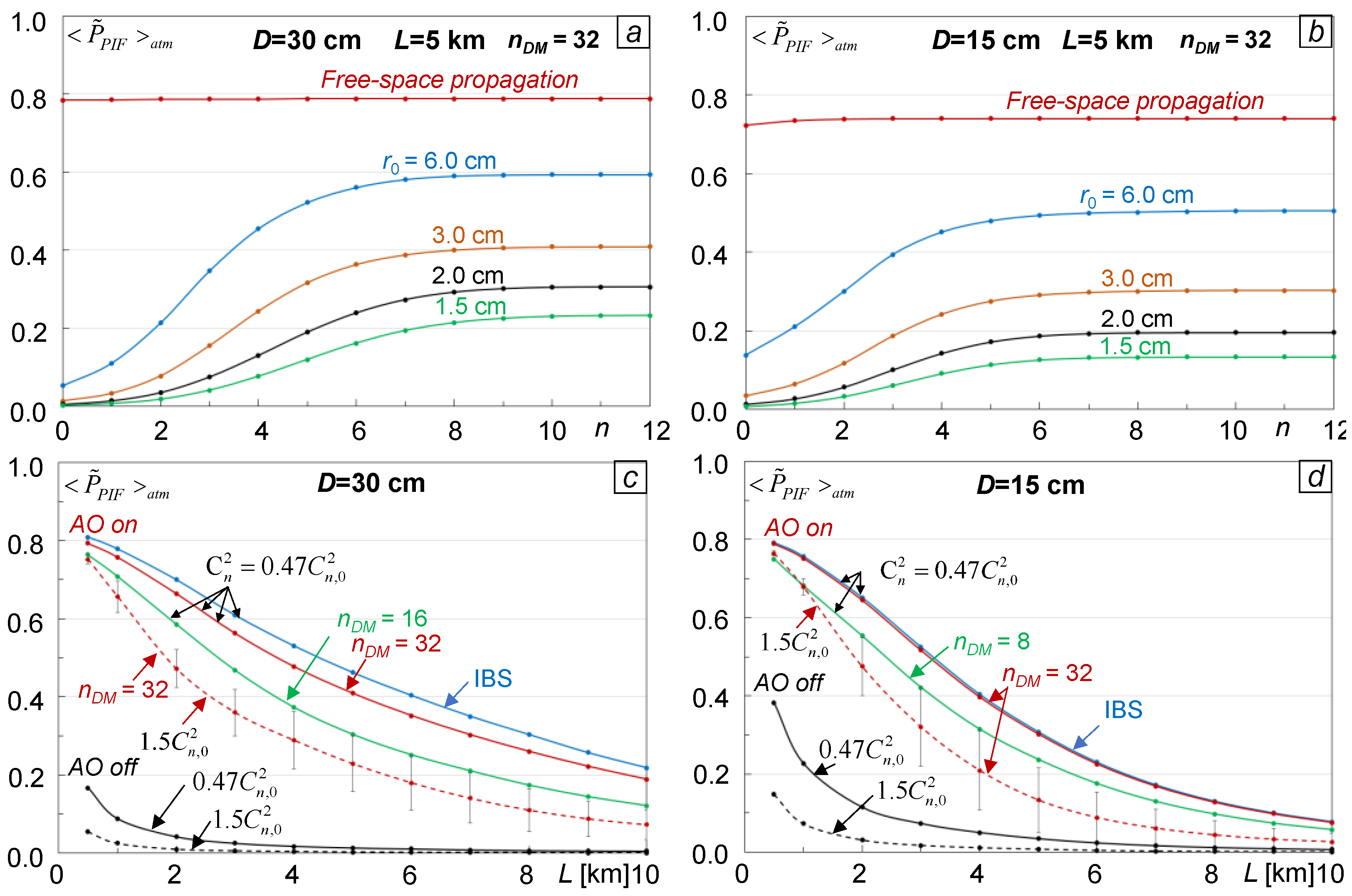
Consider how DM resolution and turbulence strength (parameters n_DM and D/r₀) impact efficiency of a laser beam projection system with SAPCO-AO based control. To address this question, we computed normalized atmospheric-averaged PIB metric values $<{\tilde{J}}_{PIB}^{dif}{>}_{atm}=<J_{PIB}(t=T_{trial}){>}_{atm}/J_{PIB}^{dif}$ corresponding to the adaptation trial end (at $t=T_{trial}=40{\tau }_{it}$) for D/r₀ ranging from zero (propagation in vacuum) to D/r₀ =20 (strong turbulence conditions) for different parameters n_DM. The normalization factor $J_{PIB}^{dif}$ describes here the diffraction-limited PIB metric value for the transmitted beam optimally focused a distance L in vacuum. The simulations were performed for the SAPCO-AO controller conducting two PR iterations per control cycle (M_PR =2). Atmospheric averaging was based on N_trial =100 computer simulated AO control trials consisting of N_update =20 control updates with an overall AO trial duration of $T_{trial}=20{\tau }_{AO}=40{\tau }_{it}$.

The M&S results are presented in Figure 6 by the dependencies $<{\tilde{J}}_{PIB}^{dif}(D/r_0){>}_{atm}$ computed for laser beam projection over distances L=5 km (a,c) and L=10 km (b,d) without (a,b) and with (c,d) tip/tilt aberration component removal prior to the adaptation trial start. Solid lines characterize performance of the SAPCO-AO control system utilizing piston DMs with different resolutions (parameter n_DM). The dashed and dotted curves in Figure 6 respectively marked as “Tip/tilt removal only” and “No DM control; No tip/tilt removal” correspond to M&S trials performed without update of DM controls: a_j(t_n)}=0, (n=0,…, N_update). In the latter case (dotted curves) tip/tilt aberration components were not removed.

Compare atmospheric-averaged PIB metric values computed for the beginning (t=0) and end (t =T_trial) of the adaptation trials (dotted and solid lines in Figure 6) with the corresponding dependencies (marked as IPC curve) obtained using the ideal phase-conjugate (IPC) control algorithm (3). The IPC curves in Figure 6 characterize the maximally achievable atmospheric-averaged PIB metric values for a specific turbulence condition (D/r₀ ratio), BD geometry, and beam projection engagement scenario. The relatively sharp decline of PIB metric values corresponding to the IPC control algorithm with D/r₀ increase, which is more noticeable at a longer (L=10 km) propagation distance, underlines the physics-based limitations of PC-based control in the mitigation of turbulence-induced phase aberrations distributed along the propagation path (volume) with a single DM.

The results presented in Figure 6 demonstrate that with utilization of a sufficiently high resolution DM, the SAPCO-AO control approach can potentially provide a laser beam projection efficiency approaching the physics-based limitation even under strong scintillation conditions (Rytov number up to ${\sigma }_R^2=8.75$ for L= 5 km and ${\sigma }_R^2=15.5$ for L= 10 km). Note that even SAPCO-AO control with relatively low resolution DMs (e.g., n_DM = 8 in Figure 6) exhibits the potential for substantial PIB metric increase when compared with the absence of AO wavefront phase aberration pre-compensation (dotted curves). Specifically, for n_DM = 8 and under turbulence strengths ranging from moderate (D/r₀ = 5) to strong (D/r₀ = 20), SAPCO-AO control can lead to atmospheric-averaged PIB metric value increases by factors ranging from approximately 3.9 to 9.2 for L = 5 km, and from 3.8 to 6.5 for L = 10 km.

The M&S results in Figure 6 (solid curves) also indicate that an increase in DM resolution beyond n_DM =32 has a relatively minor impact on the AO system performance while leading to a potentially significant increase in system complexity and cost. Similarly, the removal of tip/tilt aberration components with a BSM-based feedback control system results in only a relatively minor PIB metric increase, especially in strong turbulence and scintillation conditions. This conclusion can be derived from comparison of the corresponding dependencies $<{\tilde{J}}_{PIB}^{dif}(D/r_0){>}_{atm}$ in Figure 6 obtained for a SAPCO-AO system without (a, b) and with (c, d) tip/tilt aberration component removal. These results suggest that with utilization of a piston DM with sufficiently high resolution (e.g., with n_DM =8 or higher) a supplementary BSM-based tip/tilt control subsystem may not be required.

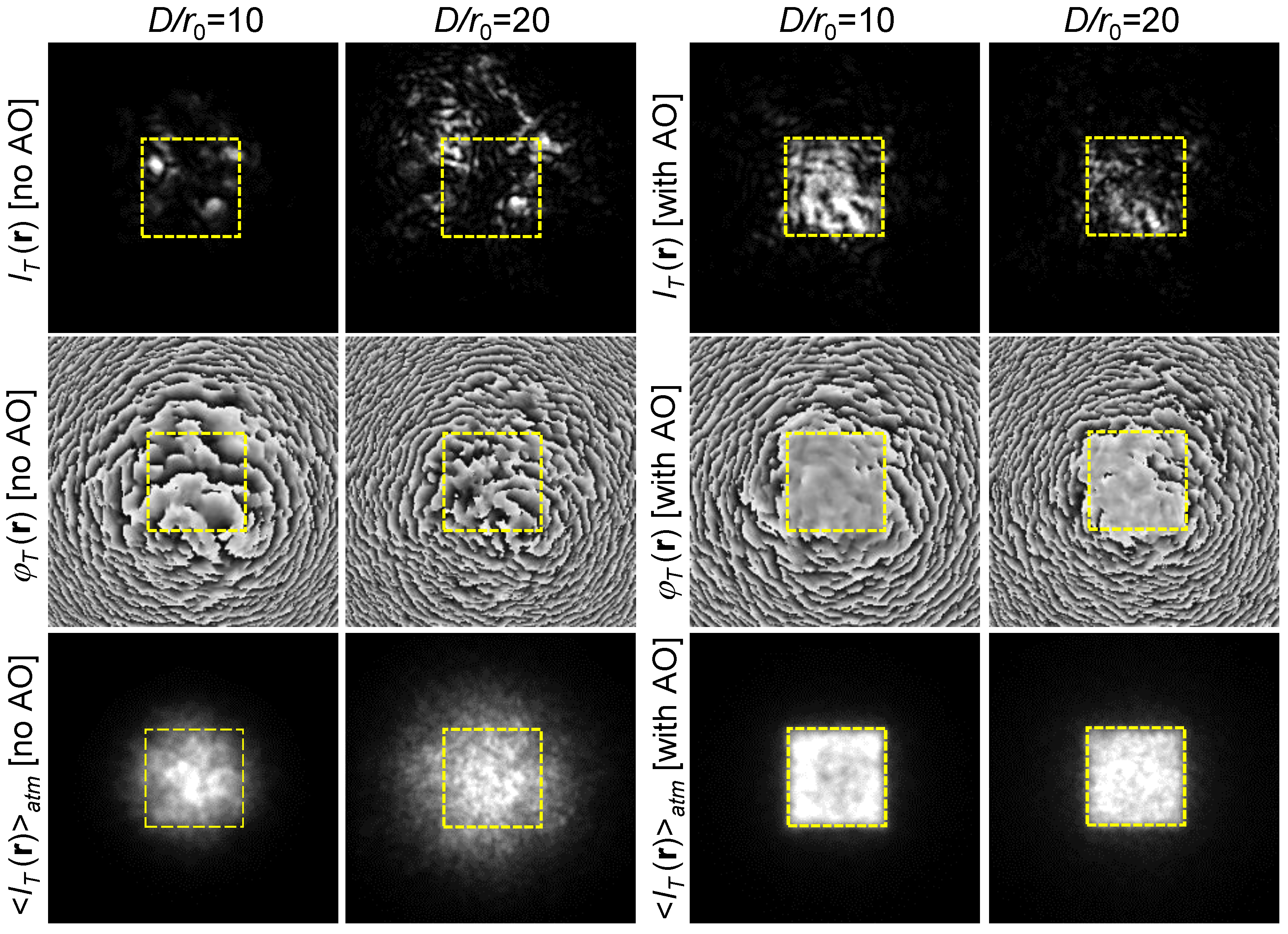
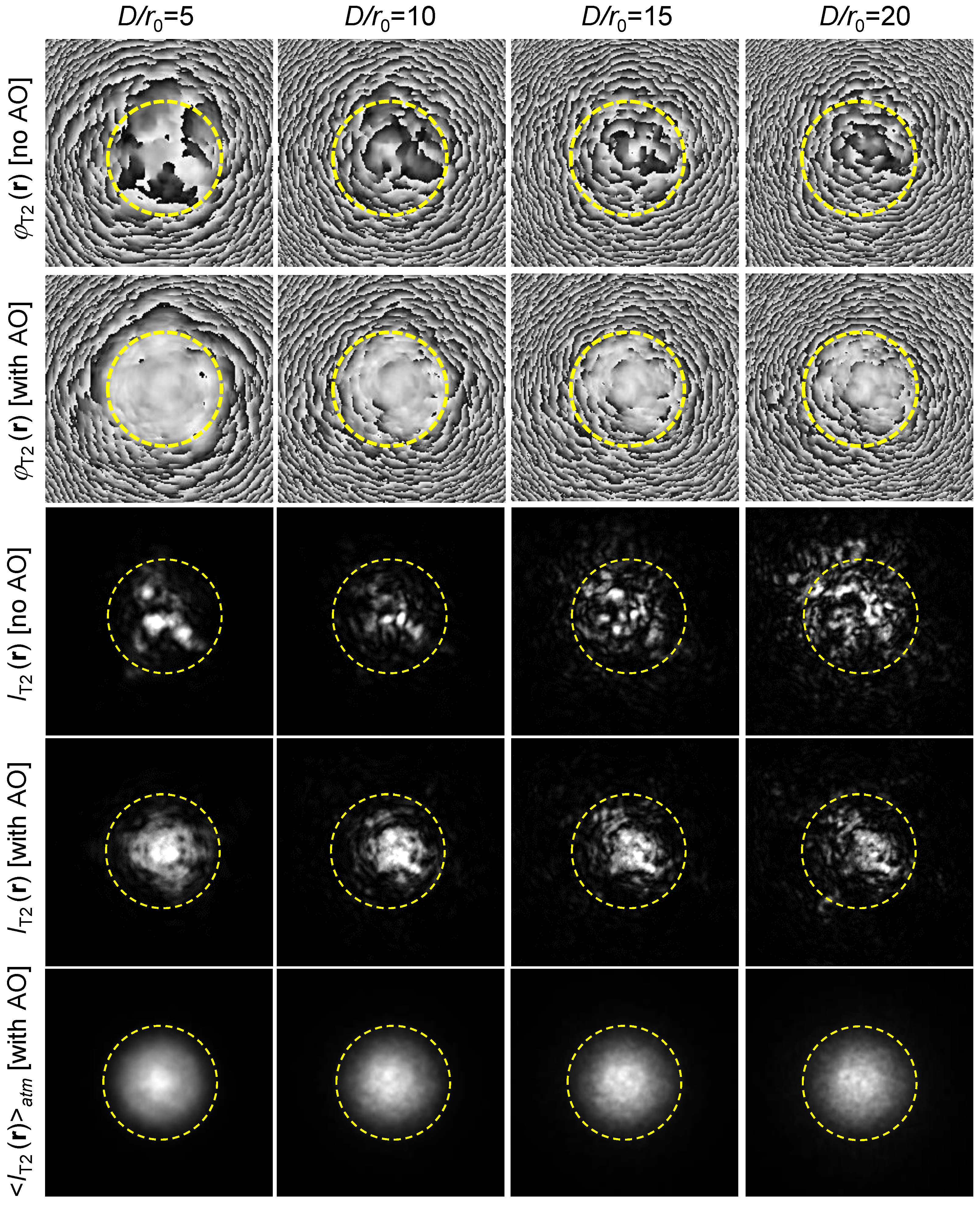
SAPCO-AO control efficiency can also be assessed by considering the grey scale images in Figure 7 computed for a characteristic (arbitrarily selected) adaptation trial and two D/r₀ ratio values. The initial (prior to first control update) intensity $I_{WFS}(r)$ and phase ${\phi }_{WFS}(r)$ distributions shown in the first two columns indicate the presence of strong intensity scintillations and turbulence-induced phase aberrations resulting in a broad spreading of the projected laser beam at the target plane. The corresponding target plane intensity distributions $I_T(r,0)=|A(r,z=L,t=0){|}^2$ computed for the optimally focused (propagation in vacuum) outgoing beam and identical turbulence realizations are shown in the third column.

The target-plane intensity distributions $I_T(r,T_{trial})$ obtained at the end of the adaptation trials (at t=T_trial) for the SAPCO-AO control system with n_DM =32 are presented by images shown in the right column. As can be seen from the target plane intensity distributions and corresponding PIB metric values ${\tilde{J}}_{PIB}^{dif}(0)$ and ${\tilde{J}}_{PIB}^{dif}(T_{trial})$ (shown in Figure 7 by inserts in the right two columns), AO control resulted in significant localization of the projected laser beam intensity distribution and corresponding PIB metric value increase (9-fold for D/r₀ =10 and by a factor of 38 for D/r₀ =20).

To conclude this efficiency analysis of the SAPCO-AO-based DE-LBP system, consider the impact of cross-wind induced effects. In the M&S we assumed an AO controller operating with a piston DM composed of N_DM =32x32 (n_DM =32) actuators. The duration of each AO control cycle was set to τ_AO = 300 μsec and included two PR iterations (M_PR=2). Each AO control trial consisted of N_update =14 control updates and atmospheric-averaging was performed over N_trial =100 adaptation trials.

Cross-wind was simulated via displacement of turbulence realizations comprised of N_φ =50 phase screens along the ox direction after each timestep. The time interval Δt between sequential timesteps was set to Δt = τ_it =133 μs. The displacement distance of each turbulence realization (measured in grid pixels) was dependent on the preset cross-wind velocity v₀.

M&S results are presented in Figure 8 by time dependencies of the normalized atmospheric-averaged PIB metric $<{\tilde{J}}_{PIB}^{dif}(t/{\tau }_{AO}){>}_{atm}=<J_{PIB}(t/{\tau }_{AO}){>}_{atm}/J_{PIB}^{dif}$ computed for horizontal (solid lines) and slant (dashed lines) propagation scenarios. Simulations were performed for laser beam projection over L= 5 km under moderate-to-strong and strong turbulence conditions corresponding to a horizontal propagation path near the ground (elevation h=0) with corresponding ground-level refractive index structure parameter values ${\mathrm{C}}_n^2\left(h=0\right)=4.7\cdot {10}^{-15}{\mathrm{m}}^{-2/3}$ for D/r₀=10 in Figure 8 (a) and ${\mathrm{C}}_n^2\left(h=0\right)=1.5\cdot {10}^{-14}{\mathrm{m}}^{-2/3}$ for D/r₀=20 in Figure 8 (b).

As expected, increases in the cross-wind velocity v₀ and/or turbulence strength resulted in an overall decline in efficiency of turbulence effects mitigation and a noticeable (especially for D/r₀ =20) increase in the AO process convergence time, as indicated by the solid lines in Figure 8. Note that laser beam projection over the horizontal path near the ground with homogeneously distributed turbulence represents perhaps the “harshest” scenario for adaptive optics.

For practical DE-LBP applications, it is more common that the laser beam is projected onto a target moving (flying) with a velocity v_T at an elevation H above the ground. Such laser beam projection engagement scenarios can be represented in numerical simulations by a model of cross-wind with a velocity linearly increasing along the propagation path (along the oz-axis) v₀(z), e.g., from v₀(z=0)=0 at the BD pupil plane to v₀(z=L)=v_T at the target plane, as in the case considered in Figure 8. For a slant propagation path, the elevation h(z) is linearly increased along the propagation path leading to a corresponding decrease in turbulence strength from the ground value ${\mathrm{C}}_n^2\left(h=0\right)$ to ${\mathrm{C}}_n^2\left(h=H\right)$, as characterized by the refractive index parameter elevation profile ${\mathrm{C}}_n^2\left(h\right)$. In the M&S we used an atmospheric turbulence structure parameter elevation profile corresponded to the Hufnagel-Valley model [31]. This turbulence strength decrease with elevation is preferred for achieving more efficient phase aberration pre-compensation with the AO-based wavefront control.

To illustrate, consider the PIB metric time-evolution curves (dashed lines in Figure 8) computed for the target at an elevation h = 500 m and distance L= 5 km moving along a trajectory orthogonal to the projected laser beam propagation path (cross-target) with velocity v_T. As can be seen from the results presented in Figure 8, with identical ground level turbulence strength [parameter $C_n^2(h=0)$] efficiency of AO control in mitigation of turbulence effects is significantly better for slant vs horizontal propagation (compare the solid and dashed curves in Figure 8).

As the M&S shows for the case considered in Figure 8, removal of tip/tilt aberrations did not noticeably change AO control performance but rather resulted in an approximately 15% decrease in the adaptation process convergence time τ_conv.

3. Remote Laser Power Transfer in a Turbulent Atmosphere with SAPCO-AO Control

3.1. Remote Laser Power Beaming: Adaptive Wavefront Control Requirements

In this section we consider application of the SAPCO-AO control concept to the problem of laser power transfer in the atmosphere to a remotely located optical-to-electrical (O-E) power converter, also referred to as remote laser power beaming (LPB) [32]. A notional schematic of a LPB system with adaptive control of the outgoing laser beam phase is shown in Figure 9. We assume here that the O-E power converter assembly consists of an optical transceiver (telescope) of diameter D concentrating laser power onto an array of densely packed square-shape photo-voltaic cells (PVC) of overall size d_PVC. The transceiver telescope pupil plane is reimaged with a coordinate scaling factor M onto the PVC array plane. To simplify notation, we consider M =1 and assume the PVC array area S_PVC =d_PVC x d_PVC is inscribed in a circular optical transceiver aperture. For practical reasons the PVC array can be illuminated by a laser beam directly (without employing an optical transceiver), or can be substituted with a fiber bundle routing the received laser power to be fanned out across remotely located PV cells.

The O-E power converter in Figure 9 includes a laser beacon unit operating at a slightly different wavelength from the projected laser beam wavelength, a beam shaper, and a dichroic beam splitter (DBS). The beam shaper (e.g., a diffractive optics element) is used to generate a laser beacon optical wave with characteristics desired for the LPB applications as discussed below (Section 3.3).

Atmospheric turbulence and platform jitter may cause undesired broadening and random wander of the transmitted laser beam footprint leading to a significant portion of the transmitted laser power missing the PVC array, causing LPB system efficiency decline. In addition to the need for keeping the laser beam within the PVC array area, for optimal power beaming system performance the received laser beam intensity distribution should be maximally uniform. This requirement is important for two reasons. First, strong intensity inhomogeneities (e.g., originating from turbulence-induced scintillations) may impose limitations on O-E power convergence efficiency, which depends on the least illuminated (“darkest”) PV cell. In operation under strong intensity scintillations this “dark-cell” bottleneck may cause significant decrease in O-E power convergence efficiency.

Second, a too bright illumination of PV cells resulting from either turbulence-induced intensity spikes or excessive laser beam power concentration within a small PVC array region can cause PV cell overheating and even damage.

These constraints distinguish the adaptive optics role in remote laser power beaming (LPB) from that for laser beam projection (DE-LBP) discussed in Section 2. Adaptive wavefront control in LPB systems, referred to here as adaptive beam shaping, aims not only to maximize the overall laser power level inside the PVC array and minimize spatial inhomogeneities in the received beam intensity, but also to mitigate turbulence-induced highly localized intensity fluctuations (intensity spikes).

Correspondingly, performance measures used for analysis of SAPCO-AO control in DE-LBP systems, such as phase error ${\epsilon }_{\delta }^{AO}(t)$[Eq. (13)] and the PIB metric $J_{PIB}(t)$ [Eq. (14)] cannot be directly applied for laser power beaming applications. Similarly, we should also reconsider the wavefront control algorithms discussed in conjunction with laser beam projection systems having SAPCO-AO control, such as the piston phase pre-compensation [Eq. (4)] and ideal phase conjugation (IPC) [Eq. (3)] algorithms - both requiring a point-source (unresolved) laser beacon for turbulence-induced aberration sensing. Despite these differences, the generic architecture of the laser beam transceiver system with SAPCO-AO control shown in Figure 1 remains applicable for remote laser power beaming with adaptive beam shaping, as discussed here.

3.2. Remote Laser Power Beaming Performance Metrics

By accounting for the LPB specific requirements mentioned above, adaptive beam shaping can be formulated in terms of minimization of the following beam shape fidelity (beam shaping) metric:

$$J_{BSM}(t)={{\displaystyle \int \left[I_T^{1/2}(r,t)-I_{ref}^{1/2}(r)\right]}}^2{d}^{2}r,$$

(15)

where $I_T(r,t)=|A(r,z=L,t){|}^2$ and $I_{ref}(r)$ are, correspondingly, the intensity distribution of the transmitted beam at the receiver telescope pupil (target) plane (z= L) and the desired (reference) intensity distribution $I_{ref}(r)$ (e.g., spatially uniform within the optical receiver aperture region associated with the PVC array area S_PVC) with a beam power identical to the projected beam power P₀.

The intensity distribution $I_T(r,t)$ in Eq. (15) corresponds to a transmitted laser beam with complex amplitude $A(r,z=0,t)=A_0(r)\exp [iu(r,t)]$ [Eq. (9)] and controllable phase $u(r,t)$ defined by Eq. (10). As in the DE-LBP application described above, propagation of the transmitted beam is described by Eq. (7).

As already mentioned, power beaming efficiency depends on the following:

(a) the overall amount of laser power delivered into the PVC receiver area (power inside the “PVC bucket” metric)

$$P_{PVC}(t)={\displaystyle \int W_{PVC}(r)I_T(r,t)}{d}^{2}r;$$

(16)

(b) spatial inhomogeneity of the laser beam intensity inside the PVC area (scintillation index)

$${\sigma }_I^2(t)={{\displaystyle \int W_{PVC}(r)\left[I_T(r,t)-{\overline{I}}_T(t)\right]}}^2{d}^{2}r/{\overline{I}}_T^2(t);\mathrm{and}$$

(17)

(c) maximum level of laser power inside a highly localized region within the PVC array, as defined by a kernel function $\rho (r,a_{sp})$ of width a_sp, which is referred to here as the intensity spike metric

$$J_{sp}(t)=\underset{r\in S_{PVC}}{\max }{\displaystyle \int \rho (r-r^{\prime },a_{sp})I_T(r^{\prime },t)}{d}^2{r}^{\prime }/{\overline{I}}_T(t),$$

(18)

where ${\overline{I}}_T(t)$ is the mean value of the intensity within the PVC receiver region described by the window function $W_{PVC}(r)$. In M&S the delta-function $\delta (r)$ was considered as the kernel function $\rho (r,a_{sp})$. In this case the spike metric (18) describes the peak intensity value inside the PVC array area.

Similar to Section 2, for an effectiveness assessment of remote power beaming with SAPCO-AO-based adaptive beam shaping we used atmospheric-averaged values of the corresponding performance metrics [Eq. (15)-Eq. (18)], which were computed for a set of N_trial =100 AO trials composed of N_update sequential DM control updates starting with identical initial conditions corresponding to $\{a_j(t_0=0)\}=0$.

3.3. Fidelity Metric Minimization via Adaptive Beam Shaping

To derive the wavefront phase control algorithm leading to minimization of the beam shaping metric (15), represent this metric in the following equivalent form:

$$J_{BSM}(t)={\displaystyle \int I_T(r,t)}{d}^{2}r{d}^{2}r+{\displaystyle \int I_{ref}(r)}{d}^{2}r-2{\displaystyle \int A(r,L,t)\psi (r,L,t_n)}{d}^{2}r,\mathrm{where}$$

(19)

$$\psi (r,L,t)=I_{ref}^{1/2}(r)\exp [-i{\phi }_A(r,t)]\mathrm{and}{\phi }_A(r,t)=\arg [A(r,L,t)].$$

(20)

Since the first two terms in Eq. (19) are independent of the controllable phase $u(r,t)$ (we assumed here optical power conservation for the transmitted laser beam), minimization of metric $J_{BSM}(t)$ with respect to the controllable phase $u(r,t)$ is equivalent to maximization of the following integral, referred to here (similar as in Part I, Ref. [1]) as the overlapping integral or interference metric [33,34]:

$$J_{int}(t)\equiv {\displaystyle \int A(r,L,t)\psi (r,L,t)}{d}^{2}r={\displaystyle \int I_T^{1/2}(r,L,t)I_{ref}^{1/2}(r)}{d}^{2}r.$$

(21)

Assume now a hypothetical reference laser source (laser beacon) located at the target plane that generates a coherent laser beam with complex amplitude defined by Eq. (20):

$$\Psi (r,L,t)=\psi (r,L,t)=I_{ref}^{1/2}(r)\exp [-i{\phi }_A(r,t)].$$

(22)

As in Section 2, the laser beacon operates at a wavelength slightly different from the projected laser beam wavelength. Propagation of the beacon beam to the laser transceiver plane (back propagation) is described by Eq. (8), where Eq. (22) represents the boundary condition.

Using Equations (9) and (8) for the counter-propagating waves with complex amplitudes $A(r,z,t)$ and $\Psi (r,z,t)$ one can derive the following relationship coupling integral characteristics of these complex amplitudes at the transmitter and PVC target planes [35]:

$${\displaystyle \int A(r,L,t)\Psi (r,L,t)}{d}^{2}r={\displaystyle \int A(r,0,t)\Psi (r,0,t)}{d}^{2}r.$$

(23)

Accounting for the boundary condition (22), from Eq. (22) we obtain:

$$J_{int}(t)={\displaystyle \int A(r,L,t)\Psi (r,L,t)}{d}^{2}r={\displaystyle \int A_0(r)I_{in}^{1/2}(r,t)\exp [iu(r,t)+i{\phi }_{in}(r,t)]}{d}^{2}r,$$

(24)

where $I_{in}(r,t)=|\Psi (r,0,t){|}^2$ and ${\phi }_{in}(r,t)=\arg [\Psi (r,0,t)]$ are intensity and phase distributions of the beacon optical wave at the BD transceiver telescope (input wave).

The right-hand side of this expression depends on the controllable phase $u(r,t)$ to be selected via maximization the overlapping integral module. As follows from Eq. (24) the maximum value of the metric |$J_{int}(t)$| leads to the following control algorithm, referred to here as ideal beam shaping (IBS):

$$u(r,t)=-{\phi }_{in}(r,t)=-[{\phi }_0(r,t)+{\phi }_{atm}(r,t)].$$

(25)

Here, the term ”ideal” is used to denote PC type wavefront control with infinitely high resolution, but not necessarily the best possible (optimal) beam shaping. For simplicity we assumed that the controllable phase modulation $u(r,t)$ in Eq. (25) includes both the atmospheric turbulence-induced ${\phi }_{atm}(r,t)$ and static ${\phi }_0(r)$ (associated with laser beacon location) phase aberration components.

The IBS control strategy [Eq. (26)] derived here is reminiscent of the ideal phase-conjugate (IPC) wavefront control algorithm (3) discussed in Section 2. The important difference between the IPC and IBS algorithms is the requirement imposed on the laser beacon. In DE-LBP applications, it is assumed that the laser beacon is unresolved so that the beacon size $d_b<d_{Airy}=2.44\lambda L/D$. In the remote power beaming application considered here the beacon beam intensity and phase profiles are prescribed by Eq. (22).

Specifically, the beacon beam intensity distribution should correspond to the spatial profile $I_{ref}(r)$ desired for optimal performance of O-E power conversion (e.g., to be uniform within the PVC target area S_PVC), and the beacon beam phase ${\phi }_{ref}(r,t)$ should be conjugated to the transmitted beam phase ${\phi }_A(r,L,t)$ at the PVC target plane: ${\phi }_{ref}(r,t)=-{\phi }_A(r,t)$. In the case of IBS control algorithm (25) the latter condition is fulfilled automatically and independently of the selected phase ${\phi }_{ref}(r,t)$. Now substitute Eq. (25) for the controllable phase $u(r,t)$ into the right-hand side of expression (24) and represent the beacon beam complex amplitude in the form $\Psi (r,L,t)=I_{ref}^{1/2}(r)\exp [i{\phi }_{ref}(r,t)]$ in the left-hand side of this expression. As a result, instead of Eq. (24) we obtain:

$${\displaystyle \int I_T^{1/2}(r,t)I_{ref}^{1/2}(r)\exp [i{\phi }_A(r,t)+i{\phi }_{ref}(r,t)]}{d}^{2}r={\displaystyle \int A_0(r)I_{in}^{1/2}(r,t)}{d}^{2}r.$$

(26)

Since the right-hand side of Eq. (26) is a real function, equality (26) can only be satisfied if the wavefront phase ${\phi }_A(r,t)$ is conjugated with respect to any pre-selected wavefront phase ${\phi }_{ref}(r,t)$ of the laser beacon beam:

$${\phi }_A(r,t)=-{\phi }_{ref}(r,t)+2\pi n,n=0,1\dots$$

(27)

This property of the transmitted beam phase rooted in the general optical reciprocity principle significantly simplifies practical implementation of remote power beaming with AO beam shaping. For optimal performance [in terms of fidelity metric (15) optimization] the E-O power converter assembly, such as shown in Figure 1 (insert), should enable generation of a laser beacon beam with the desired (e.g., spatially uniform) intensity distribution $I_{ref}(r)$ within the PVC target. The laser beacon wavefront phase can be static ${\phi }_{ref}(r,t)={\phi }_{ref}(r)$ and can be selected based on practical considerations, e.g., ${\phi }_{ref}(r)=const$, as in the case of a collimated beacon beam. Such a laser beacon (specific for each selected PVC target geometry) can be formed using specially designed beam shaping optical elements (e.g., DOE-based). To distinguish between laser beacons in laser beam projection (DE-LBP) and laser power beaming (LPB) applications, the latter specially designed (pre-shaped) laser reference source is referred to here as a PS-beacon.

3.4. Remote Power Beaming with Adaptive Beam Shaping: Numerical Simulation Results

In performance analysis of adaptive beam shaping, we used major M&S parameters identical to those in Section 2 for the beam director (BD) and SAPCO-AO control subsystems, including BD aperture (D=30 cm), piston DM resolution (n_DM =32), and the number of phase retrieval (PR) iterations per control cycle (M_PR=2).

A square PVC array (PVC target) of size d_PVC (ranging from 0.5 d_Airy to 10.0 d_Airy) was located a distance L = 5 km in homogeneously distributed turbulence represented by N_φ= 50 equally spaced Kolmogorov phase screens. The projected laser beam with super-Gaussian intensity distribution was initially (prior to the first DM control update) focused a distance ΔL=d_PVC L /(D-d_PVC) behind the PVC target. In the geometrical optics approximation such initial beam focusing a distance L+ΔL corresponds to a beam footprint diameter matching the PVC target size d_PVC. The PS-beacon beam was represented in M&S by a collimated [${\phi }_{ref}(r)=0$] laser beam with square super-Gaussian (power eight) intensity distribution of size d_b = d_PVC.

Due to the direct similarity between the IPC [Eq. (3)] and IBS [Eq. (26)] control algorithms, adaptive beam shaping using a piston DM (n_DM =32) was performed by utilizing the PC-type control algorithm Eq. (4), where expression (6) was used for computation of piston phases. As in Section 2, atmospheric averaging was performed based on N_update =100 adaptation (beam shaping) trials.

The impact of adaptive beam shaping can be qualitatively assessed by considering the intensity $I_T(r)=|A(r,L){|}^2$ and phase ${\phi }_T(r)\equiv {\phi }_A(r)=\arg [A(r,L)]$ distributions (intensity and phase patterns) at the PVC target plane (z=L) computed for moderate-to-strong (D/r₀ =10) and strong (D/r₀ =20) turbulence conditions, as shown in Figure 10. The intensity and phase patterns in the top two rows correspond to the start (labeled as “no AO”) and end (labeled as “with AO”) of a characteristic adaptation trial comprised of N_update =12 sequential DM control updates (control cycles). The corresponding atmospheric-averaged intensity patterns are shown in the bottom row. The intensity patterns in Figure 10 (in particular, the atmospheric-averaged patterns in the bottom row) clearly demonstrate the ability of the SAPCO-AO control to shape the intensity distribution to the specific geometry of the PVC array (square).

Consider now the impact of adaptive beam shaping on wavefront phase patterns at the PVC target plane (middle row images in Figure 10). First, note that, as shown in Section 3.3, ideal beam shaping [Eq. (25)] results in the formation of the target plane optical wave $A(r,L)$ with wavefront phase ${\phi }_T(r)=\arg [A(r,L)]$ conjugated with respect to the PS-beacon beam phase ${\phi }_{ref}(r)$ [see Eq. (27)]. Correspondingly, in the case considered here [a collimated square-shaped PS-beacon beam and high resolution (n_DM =32) piston DM], it is expected that adaptive beam shaping results in mitigation of the spatial non-uniformity (flattening) of the target plane phase ${\phi }_T(r)$ inside the beacon beam footprint area.

This flattening of the projected laser beam phase at the PVC target region can be clearly seen from the phase images when we compare phase patterns, corresponding to the adaptation trial beginning and end, in Figure 10 (middle row). Despite the significant overall reduction in the spatial nonuniformity level, the phase patterns resulting from adaptive beam shaping (right two images in the middle row) still display presence of branch points and phase cuts.

For a qualitative performance assessment of SAPCO-AO-based adaptive beam shaping, consider the dependencies of atmospheric-averaged laser power beaming performance metrics [Eq. (15)-Eq. (18)] on the number n of sequential control updates, as shown in Figure 11. Metrics were computed for a set of N_trial =100 adaptation trials composed of N_update = 12 control updates and identical initial conditions:$\{a_j(n=0)\}=0,$ (j=1,…, N_DM).

Notice the non-monotonic character of the dependencies $<{\tilde{J}}_{BSM}(n){>}_{atm}$ in Figure 11 (a). Despite of the anticipated monotonic decline of the beam shaping fidelity metric $<{\tilde{J}}_{BSM}{>}_{atm}$ for the IBS-type control algorithm [Eq. (25)], numerical simulations show the metric values increase during the first two or three control updates, dependent on the parameter D/r₀. Similar non-monotonic behavior is observed for the metric $<{\tilde{P}}_{PVC}(n){>}_{atm}$ (power inside “PVC bucket”) in Figure 11 (b)

As the numerical simulations show, such “unexpected” non-monotonic behavior of both metrics is related with residual digital noise in the retrieved phase that is still present after the first few M_PR PR iterations (e.g., for M_PR =2 in Figure 11), as discussed in Section 2.5. This noise “propagates” into the DM controls, resulting in the appearance of high frequency phase aberration components and a corresponding broadening of the target plane intensity distribution as shown by the middle (n=2) image in Figure 11 (c). As already mentioned in Section 2.5, the digital noise amplitude gradually decreases with either an increase in the number of PR iterations (parameter M_PR) per AO cycle, or number of performed DM update cycles n, or both. To confirm the origin of the non-monotonic behavior of metrics $<{\tilde{J}}_{BSM}{>}_{atm}$ and $<{\tilde{P}}_{PVC}{>}_{atm}$, the parameter M_PR was increased from M_PR =2 to M_PR =20, which resulted in monotonic metric $<{\tilde{J}}_{BSM}(n){>}_{atm}$ decline, and metric $<{\tilde{P}}_{PVC}{>}_{atm}$ rise with n increase, as illustrated in Figure 11 (a) by the dashed line. As already discussed in Section 2.2, parameter M_PR increase is not generally desired as it leads to a corresponding decrease in the closed-loop control frequency bandwidth.

The plots presented in Figure 11 (a) show a factor of 1.2 - 1.7 (dependent on parameter D/r₀) improvement in the beam shaping fidelity metric $<{\tilde{J}}_{BSM}(n){>}_{atm}$ at the adaptation trial end (at n=12) compared with the corresponding initial metric values at n=0. The corresponding plots for the metric $<{\tilde{P}}_{PVC}(n){>}_{atm}$ in Figure 11(b) exhibit a relatively small overall metric increase (about 1.5-fold for D/r₀ =20) occurring only under moderate-to-strong and strong turbulence conditions. The adaptive beam shaping even results in a minor decrease in the power inside the PVC area under weak turbulence (D/r₀ =5) and for propagation in a vacuum (D/r₀ =0).

Adaptive beam shaping affects the scintillation index $<{\sigma }_I^2{>}_{atm}$ and intensity spike metric $<J_{sp}{>}_{atm}$ more distinctly, as illustrated by the corresponding plots in Figure 11 (c) and (d). Decline in the scintillation index resulting from adaptive beam shaping ranges from 2.4-fold for D/r₀ =20 to 3.9-fold for D/r₀ =10. The corresponding decline factor for the spike metric $<J_{sp}{>}_{atm}$ ranges from 1.7 (D/r₀ =0) to 2.6 (D/r₀ =10). Note that the scintillation index prior to adaptive beam shaping is the highest $[<{\sigma }_I^2(n=0){>}_{atm}$=2.6] for D/r₀ =10 and smaller [$<{\sigma }_I^2(n=0){>}_{atm}$=2.3] under stronger turbulence conditions (for D/r₀ =10), which can be explained by the saturation of intensity fluctuations occurring under strong turbulence conditions [36].

To conclude this analysis of remote power beaming with SAPCO-AO control, consider dependencies of the atmospheric-averaged performance metrics [Eq. (15) - Eq. (18)] in adaptation trial beginning (AO off) and end (AO on) on the PVC target size d_PVC (normalized by the Airy disk diameter d_Airy), which are presented in Figure 12. As can be seen from Figure 12 (a), adaptive beam shaping results in metric $<{\tilde{J}}_{BSM}{>}_{atm}$ decline with d_PVC increase but only until the PVC target size reaches the threshold value $d_{PVC}^{th}\simeq 6d_{Airy}$. With further d_PVC increase the beam shaping fidelity metric stagnates and even slightly increases.

On the other hand, the overall laser power received by the PVC target [metric $<{\tilde{P}}_{PVC}{>}_{atm}$ curves in Figure 12 (b)] steadily increases with d_PVC, but the initial (for d_PVC not exceeding d_Airy ) gain from utilization of adaptive beam shaping monotonically declines and practically vanishes with d_PVC >$d_{PVC}^{th}$. For an unresolved (d_PVC < d_Airy ) PVC target and, hence, with the use of an unresolved laser beacon (d_b =d_PVC), the adaptive beam shaping for laser power beaming applications considered here evolves into the AO control for the laser beam projection application discussed in Section 2.

This decline in power beaming efficiency with increases in the PVC target size observed in M&S is also illustrated by the grey-scale images of the atmospheric-averaged intensity distributions shown in Figure 12 (a), (b). The ability of AO control to shape the transmitted beam footprint into the PVC target shape can be clearly seen in these images only for d_PVC = 2.0 d_Airy and d_PVC = 4.0 d_Airy. The beam shaping capability is less pronounced for d_PVC = 6.0 d_Airy (especially noticeable in the vicinity of the PVC target corners) and is practically absent for d_PVC = 8.0 d_Airy. Such a decline in adaptive beam shaping efficiency with the PVC target and, hence, increases in the PS-beacon size, can be associated with the impact of anisoplanatic effects on beacon beam propagation through volume turbulence [37,38,39]. Under the anisoplanatic conditions that are characteristic of extended PS-beacon sizes, phase aberration components associated with distant PS-beacon regions and corresponding propagation paths can be noticeably different and, hence, cannot be fully compensated [38,39].

To a lesser degree, PS-beacon anisoplanatism negatively impacts adaptive beam shaping performance in reducing laser beam intensity spatial non-uniformities (scintillation index $<{\sigma }_I^2{>}_{atm}$), and the mitigation of intensity spikes (spike metric $<J_{sp}{>}_{atm}$) inside the PVC target region, as illustrated by the corresponding plots in Figure 12 (c) and (d). Adaptive beam shaping results in a scintillation index decrease correspondingly up to a factor 3.0 for d_PVC = 6.0 d_Airy with a corresponding drop in the spike metric by 2.3-fold.

Adaptive beam shaping still provides a noticeable decrease in both $<{\sigma }_I^2{>}_{atm}$ and $<J_{sp}{>}_{atm}$ metric values even for PVC targets of size d_PVC $\simeq$ 9.0 d_Airy (or, equivalently d_PVC $\simeq$$1.5d_{PVC}^{th}$) while advantages in using beam shaping vanishes with respect to the metrics $<{\tilde{J}}_{BSM}{>}_{atm}$ and $<{\tilde{P}}_{PVC}{>}_{atm}$.

This ability of adaptive beam shaping to reduce scintillations and intensity spikes even under strong anisoplanatic conditions can be associated with flattening of the wavefront phase for the projected laser beam at the PVC target under IBS control, previously discussed in conjunction with Figure 10 (middle row). Mitigation of turbulence-induced phase aberrations along the propagation path leading to flattening of the transmitted beam phase at the PVC target area also results in a weakening of intensity scintillations originating from the diffraction-induced transformation of phase aberrations into spatial modulation of the propagating beam intensity distribution.

4. SAPCO-AO Control-Enhanced Free-Space Optical (FSO) Communications

4.1. Bidirectional FSO Communication Link with SAPCO-AO Control: System Architecture

The successful extension of FSO communications to a wide range of ground-to-ground, ground-to-air, and ground-to-space applications is contingent to a great degree on the ability of these communication links to operate under strong turbulence conditions characterized by severe phase aberrations and intensity scintillations [6,40,41,42,43]. In this section we consider possible applications of SAPCO-AO-based turbulence mitigation techniques to atmospheric bidirectional FSO links.

A notional schematic of the bidirectional FSO communication system considered here comprised of two monostatic optical transceiver terminals (T1 and T2) is illustrated in Figure 13. It is assumed that monochromatic (or quasi-monochromatic) laser beams in these terminals are generated by utilizing laser sources with slightly different wavelengths, thus enabling separation of the transmitted and received optical waves with dichroic beam splitters (DBSs). The generated laser beams in both FSO terminals are coupled into single mode fibers (SMFs) and after propagation through fiber-optics trains (not shown in Figure 13) are emitted to free space through fiber tips. These beams represent the SMF principal eigenmodes, having a Gaussian shaped intensity and spatially uniform (plane) wavefront phase. Due to diffraction the beams are expanded, and after collimation by lenses L_c the corresponding (identical for both FSO terminals) Gaussian beams of width w are directed into free-space optical trains. For simplicity, we assumed here that all lenses (L_C and L_F) in Figure 13 have identical focal lengths and a diameter d_L >> w, and are designed to provide optimal coupling of the collimated Gaussian beam of width w into the SMFs utilized in both FSO terminals. Note that in the case of FSO terminals with transceiver telescopes (beam directors) of different aperture diameters, optimal receive laser beam coupling into the SMFs may require collimating and focusing lenses having different focal distances.

The optical train of FSO terminal T1 in Figure 13 incorporates the SAPCO-AO control system shown in Figure 1, where the laser module is substituted by a SMF-coupled laser and lens L_C. A collimated Gaussian beam entering the optical train of this terminal undergoes a controllable phase modulation $u(r,t)$ imposed by the DM and, after enlargement in size by a factor M₁ by the beam director (BD₁), is transmitted over a distance L to the remotely located FSO terminal T2.

The laser beam sent from terminal (T2) enters the BD₁ aperture, propagates through the SAPCO-AO optical train in inverse direction, and is focused to the tip of the SMF located at the lens L_F focus, as shown in Figure 13. The received optical wave power P₁(t) that is coupled into the fiber-optics train through the tip of the SMF is registered by a photo-detector (PD₁). The detected signal represents an efficiency measure commonly used in FSO communications, referred to here as the power-in-the-fiber (PIF) metric. Note that the same SMF can be utilized to transmit and receive laser beams. Separation of the counter-propagating optical waves is performed in this type of FSO communication terminals using fiber-integrated DBSs (e.g., add-drop multiplexers) and/or fiber-optics circulators [44].

The FSO terminal T2 at the other end of the bidirectional link represents the passive (without AO capabilities) optical transceiver system illustrated in Figure 13 (bottom right insert). In this system the laser beam is emitted from the SMF tip and collimated by lens L_C. After reflection from a DBS, the collimated Gaussian beam is sent into the beam director BD₂ and after enlargement by a factor M₂ is transmitted towards the FSO terminal T1. The same beam director is used to receive the laser beam from the FSO terminal T1. The received laser light passes through the DBS and after focusing by the lens L_F is coupled into the SMF. The corresponding PIF signal P₂(t) is measured by the photo-detector PD₂.

The complex amplitudes of the transmitted laser beams at the pupil planes of the corresponding FSO terminals in Figure 13 can be represented in the form:

$$A(r,z=0,t)\equiv A(r,0,t)=W_1(r)A_0(M_{1}r)\exp [iu(r,t)]\mathrm{for}\mathrm{the}\mathrm{terminal}T1,\mathrm{and}$$

(28)

$$\Psi (r,z=L)\equiv \Psi (r,L)=W_2(r)A_0(M_{2}r)\exp [i{\phi }_2(r)]\mathrm{for}\mathrm{FSO}\mathrm{terminal}T2.$$

(29)

Here $W_1(r)$ and $W_2(r)$ are step-wise functions describing transceiver apertures of the corresponding beam directors of diameters D₁ and D₂, $A_0(r)$ is the magnitude of the collimated Gaussian laser beam of width $w$ at the BD₁ and BD₂ transceiver entrance planes, and ${\phi }_2(r)$ is wavefront phase of the laser beam transmitted by the terminal T2. The BD transceiver apertures clip a portion of the transmitted laser power. In the M&S we consider an identical clipping factor $\gamma =w/D_1=w/D_2=0.89$ for both BD transceivers, which corresponds approximately to an 8% laser power loss.

4.2. Power-in-the-Fiber (PIF) Metrics in a Bidirectional FSO Link

The PIF signals P₁(t) and P₂(t) measured by the photo-detectors PD₁ and PD₂ in Figure 13 are proportional to the laser powers coupled into the corresponding SMFs and can be presented in the following form [45,46]:

$$P_1(t)=c_1{\left|{\displaystyle \int M_0(r){\Psi }_F(r,t)d^{2}r}\right|}^2,$$

(30)

$$P_2(t)=c_2{\left|{\displaystyle \int M_0(r)A_F(r,t)d^{2}r}\right|}^2.$$

(31)

Here c₁ and c₂ are parameters dependent on photo-detector sensitivities, $M_0(r)$ is a Gaussian function of width d_SMF defined by the mode field diameter of the SMF principal eigenmode, and ${\Psi }_F(r,t)$ and $A_F(r,t)$ are the complex amplitudes of the received optical waves at the focal planes of the corresponding collimating lens.

As shown in Ref [47], the integrals in Eq. (30) and Eq. (31) can be expressed through the complex amplitudes of the counter-propagating waves at the pupil planes (z=0 and z=L) of the FSO terminals and the laser powers P_T1 and P_T1 transmitted through the SMFs:

$$P_1(t)={\eta }_1{\left|{\displaystyle \int A(r,0,t)\Psi (r,0,t)d^{2}r}\right|}^2,$$

(32)

$$P_2(t)={\eta }_2{\left|{\displaystyle \int A(r,L,t)\Psi (r,L,t)d^{2}r}\right|}^2,$$

(33)

where η₁= c₁/P_T1 and η₂= c₂/P_T2. We assumed here an identical propagation path length between the SMF tips and BD exit planes for both FSO terminals, which automatically occurs when a single SMF is used to transmit and receive laser light.

As in Section 3.3, by utilizing Eq. (9) and Eq. (8) one can derive an expression analogous to Eq. (23) that links characteristics of the complex amplitudes in Eq. (32) and Eq. (33) at both ends of the FSO link. Correspondingly, from Eq. (23) and Eq. (32) and Eq. (33), we obtain [47]:

$$P_1(t)=({\eta }_1/{\eta }_2)P_2(t).$$

(34)

Equality (34) suggests that in a bidirectional FSO link that utilizes SMF for both laser beam transmission and received light power measurements, the PIF signals registered at both communication link ends are perfectly correlated even in the presence of turbulence-induced optical inhomogeneities along the propagation path [47]. Note that mismatch between optical path lengths of the counter-propagating waves, e.g., in the case of FSO terminals with different BD aperture sizes and unequal focal lengths for the collimating and focusing lenses, results in a decorrelation of the PIF signals. This decorrelation is stronger in more severe turbulence conditions [47].

The strong (ideally 100%) correlation between PIF metric values measured at both ends of bidirectional FSO links is principally important from an AO viewpoint, as it enables performance evaluation of the AO system and overall FSO link based on PIF metric measurements conducted at a single FSO terminal.

4.3. PIF Metric Optimization via Adaptive Beam Shaping

The wavefront control problem in SFO communications can be formulated in terms of fidelity (beam shaping) metric minimization, similar to what was discussed in conjunction with laser power beaming applications in Section 3. To elaborate, consider the following [analogous to Eq. (15)] beam shaping metric defined here for the BD₂ pupil plane (z=L) of FSO terminal T2:

$$J_{FSO}(t)={{\displaystyle \int \left[I_{T2}^{1/2}(r,t)-I_{ref}^{1/2}(r)\right]}}^2{d}^{2}r,$$

(35)

where $I_{T2}(r,t)=|A(r,L,t){|}^2$ and $I_{ref}(r)$ is a desired (reference) intensity distribution.

Using analogous derivations to those performed for the beam shaping metric [Eq. (15)] in Section 3.3, it can be shown that minimization of the metric $J_{FSO}(t)$ with respect to the controllable phase $u(r,t)$ is equivalent to maximization of the PIF signal $P_2(t)$[Eq. (33)], which can be achieved using the ideal beam shaping (IBS) algorithm (25).

As previously discussed, utilization of the IBS control algorithm requires generation of a reference laser beam at the BD₂ pupil plane, referred to in Section 3.3 as the PS-beacon beam, having complex amplitude ${\Psi }_{ref}(r,L)=I_{ref}^{1/2}(r)\exp [i{\phi }_{ref}(r)]$ where ${\phi }_{ref}(r)$ is the beacon beam wavefront phase.

In the beam shaping application considered in Section 3.3 the phase ${\phi }_{ref}(r)$ does not need to be specified and can be selected based on practical considerations. This is not the case for adaptive beam shaping for FSO communications, where the PS-beacon phase ${\phi }_{ref}(r)$(desired or reference wavefront phase) should be determined based on the requirement for optimal received optical wave coupling into the SMF of FSO terminal T2.

Based on optical reciprocity considerations, the optimal received light power coupling into the SMF is expected for a reference optical field with complex amplitude $A_{ref}(r,L)=\Psi *(r,L)$ conjugated with respect to the complex amplitude $\Psi (r,L)$[Eq. (29)] of the laser beam transmitted through FSO terminal 2. This implies that the pre-shaped PS-beacon beam that satisfies the requirement for the optimal received optical wave coupling into the SMF coincides with the laser beam transmitted by FSO terminal T2. These arguments enable specification of both the desired (reference) intensity $I_{ref}(r)=W_2(r)A_0^2(M_{2}r)$ and phase ${\phi }_{ref}(r)={\phi }_2(r)$ distributions.

As follows from the analysis in Section 3.3, utilization of IBS control algorithm (25) leads to shaping of the received optical field complex amplitude $A(r,L,t)$ inside the BD₂ aperture intended to match [in terms of the fidelity metric $J_{FSO}(t)$ in Eqn. (35)] the received field intensity $I_{T2}(r,t)=|A(r,L,t){|}^2$ to the reference intensity $I_{ref}(r)=W_2(r)A_0^2(M_{2}r)$. IBS control also results in the desired transformation of the received optical field phase ${\phi }_A(r,L,t)=\arg [A(r,L,t)]$ into the phase ${\phi }_{T2}(r,t)\equiv {\phi }_A(r,t)=-{\phi }_2(r)+2\pi n$ conjugated with respect to the phase of the transmitted (reference) beam, as described by Eq. (27). In the case of a collimated beam transmitted by FSO terminal T2 (collimated PS-beacon) [${\phi }_2(r)=const$] IBS control leads to flattening of the received optical wave phase: ${\phi }_{T2}(r,t)=-{\phi }_2(r)=const$.

The changes prompted by IBS control in the intensity and phase of the optical field received by FSO terminal 2 leads to the desired increase in received laser power coupling into the SMF and a corresponding maximization of the PIF signal $P_2(t)$. By considering correlation between PIF signals measured at both ends of the bidirectional FSO link [Eq. (34)], IBS control also results in maximization of the PIF signal $P_1(t)$.

This analysis of IBS control may raise a question regarding the need for AO control at both ends of SMF-based bidirectional FSO communication links. Installation of an additional AO control system at FSO terminal T2 (AO_T2) may be beneficial for increasing overall laser power inside the BD₁ transceiver aperture through better transmitted laser beam focusing inside the BD₁ transceiver aperture, but may not be advantageous for mitigation of turbulence-induced aberrations since WFS of the additional AO system (AO_T2 ) will operate with the already compensated (nearly flat for the collimated beam) wavefront phase ${\phi }_{T2}(r,t)=-{\phi }_2(r)+2\pi n$ of the received optical wave. In addition, both AO systems (AO_T1 and AO_T2) of the corresponding FSO terminals may interfere with each other making the control problem even more complicated. Certainly the above conclusion, which is based on the analysis of an idealized model for SMF-based bidirectional FSO terminals and the assumption of ideal beam shaping (IBS algorithm), requires further inquiry in order to be considered for practical FSO communication links. This analysis is beyond the scope of the current study.

4.4. FSO Communication Links with Adaptive Beam Shaping: Numerical Simulation Results

For comparison of SAPCO-AO control efficiency in FSO communications vs DE laser beam projection and remote power beaming applications discussed previously, in numerical analysis of the bidirectional FSO link we considered a similar atmospheric propagation geometry and major system parameters. The latter include laser wavelength (λ=1064 nm), propagation distance (ranging from L=0.5 km to L=10 km), turbulence characteristics (homogeneously distributed Kolmogorov turbulence with ${\mathrm{C}}_n^2=4.7\cdot {10}^{-15}{\mathrm{m}}^{-2/3}$ and ${\mathrm{C}}_n^2=1.5\cdot {10}^{-14}$m^-2/3), resolution of piston DM (n_DM =32), and the number of PR iterations per control cycle (M_PR=2). For L =5 km the selected ${\mathrm{C}}_n^2$ values correspond to the turbulence strength parameters D/r₀ = 10 and D/r₀ = 20 previously used in the M&S. As in Section 2 and Section 3, adaptive wavefront control (adaptive beam shaping) was performed based on control algorithm Eq. (4), where Eq. (6) was applied for computation of piston phases. The controllable phase $u(r)$ was defined by Eq. (10) with $u_{BSM}(r,t)=0$ (no tip/tilt control).

To simplify the analysis, we assumed that beam directors of both FSO terminals in Figure 13 transmit identical laser power P₀ and have equal aperture diameter (D₁ = D₂ =D). Wavefront phase of the beam transmitted by FSO terminal T2 was considered spatially uniform: ${\phi }_2(r)=\arg [\Psi (r,L)]=const$, which corresponds to a collimated laser beam.

FSO link efficiency was characterized using the following normalized PIF metric proportional to the signal $P_2(t)$ [Eq. (33)]:

$${\tilde{P}}_{PIF}(t)={\left|{\displaystyle \int A(r,L,t)\Psi (r,L,t)d^{2}r}\right|}^2/(P_{SMF}{P}_0),$$

(36)

where P_SMF = P_T1= P_T2 is laser power emitted through the SMF tip at both FSO terminals. To investigate the correlation between PIF signals $P_1(t)$ and $P_2(t)$ measured at opposite ends of the FSO communication link and thus to examine the validity of equality (34), we also computed the normalized PIF metric [similar to Eq. (36)] proportional to signal $P_1(t)$ [Eq. (32)] defined through the complex amplitudes $A(r,0,t)$ and $\Psi (r,0,t)$ of the counter-propagating optical waves at the BD₁ pupil plane (z=0). As expected, the normalized PIF metric values computed for both propagation path ends coincided in all conducted numerical simulations.

In the M&S it was convenient to represent ${\tilde{P}}_{PIF}(t)$ in Eq. (36) as a function of the number n of sequential control signal updates [${\tilde{P}}_{PIF}(n)$], (n=0,1…, N_update) or timesteps t_n = nτ_AO of the AO control cycle [${\tilde{P}}_{PIF}(t_n)$]. Atmospheric-averaged PIF metric values $<{\tilde{P}}_{PIF}(n){>}_{atm}$ [or ${\tilde{P}}_{PIF}(t_n)$] were computed for the set of N_trial =100 AO trials composed of N_update =12 sequential DM control updates starting with identical initial conditions corresponding to $\{a_j(t_0=0)\}=0$.

The impact of adaptive beam shaping on the intensity $I_{T2}(r)=|A(r,L){|}^2$ and phase ${\phi }_{T2}(r)=\arg [A(r,L)]$ of the optical field entering FSO terminal T2 at the beginning [no AO] and end [with AO] of a selected adaptation trial is illustrated in Figure 14 for different D/r₀ ratio values. Numerical simulations were conducted for a FSO link of L=5 km length. As can be seen from a comparison of the corresponding phase and intensity patterns, AO control results in both wavefront phase ${\phi }_{T2}(r)$ flattening and intensity distribution $I_{T2}(r)$ centering inside the BD₂ aperture area. These AO-induced changes in phase and intensity spatial structure provide the desired increase in laser power coupling into the SMF with a corresponding gain in the PIF metric. When turbulence strength (parameter D/r₀) increases, wavefront phase flattening is less pronounced and occurs over smaller area. In addition, phase patterns inside the aperture area become more and more corrupted by the presence of a growing number of wavefront phase singularities (branch points and 2π phase cuts), as can be seen in Figure 14 (second row). Further potential SFO link performance enhancement is related with mitigation of these wavefront phase singularities, e.g., using an additional adaptive optics system installed at FSO terminal T2, which nevertheless represents an extremely challenging task for conventional AO. Furthermore, as already mentioned, AO control systems installed at both ends of the FSO link may affect each other. Stability and efficiency of such two-component AO control requires separate study.

Consider now the intensity patterns presented in Figure 14. Parameter D/r₀ increase results in a general rise of intensity scintillations for operation with and without AO control. Nevertheless, scintillation strength is noticeably smaller in the case of adaptive beam shaping (compare the corresponding intensity patterns in Figure 14).

The ability of the SAPCO-AO control to shape the intensity distribution aiming to optimally replicate the intensity profile of the transmitted laser beam within the BD₂ aperture area is illustrated by the atmospheric-averaged intensity patterns in the bottom row in Figure 14. Simulation results show that for all D/r₀ parameter values considered in the M&S, the atmospheric-averaged intensity patterns $<I_{T2}(r){>}_{atm}$ quite well approximate the shape of the transmitted clipped Gaussian beam.

SAPCO-AO control efficiency in a bidirectional FSO communication link was evaluated in M&S using the atmospheric-averaged normalized PIF metric $<{\tilde{P}}_{PIF}{>}_{atm}$ as defined by Eq. (36). Numerical simulation results computed for FSO communication links with BD aperture diameters D = 30 cm and D =15 cm are presented in Figure 15. M&S was performed for different propagation lengths L, turbulence strengths as characterized by the refractive index structure $C_n^2$ and Fried $r_0={(0.16C_n^2{k}^{2}L)}^{-3/5}$ parameters, and for a SAPCO-AO control system utilizing piston DMs of different resolutions (parameter n_DM).

Evolution of the atmospheric-averaged PIF metric $<{\tilde{P}}_{PIF}{>}_{atm}$ values during sequential control updates computed for the propagation length L=5 km in vacuum (free-space propagation) and in atmospheric turbulence conditions with different Fried parameters r₀ is illustrated in Figure 15 (a),(b). For all parameters considered, the AO process converged after eight to ten control updates, dependent on r₀ and D. This convergence rate corresponds to the closed-loop AO system frequency bandwidth f_AO ~ 0.5 - 0.4 kHz. Here, as in Section 2.5, we considered M_PR=2, n_DM=32 and used τ_it =133 μs as a reference.

As seen from the PIF metric evolution curves in Figure 15 (a), (b) efficiency of adaptive beam shaping rapidly declines with turbulence strength increase (r₀ decrease). When compared, the PIF metric values $<{\tilde{P}}_{PIF}(N_{update}){>}_{atm}$ achieved during the adaptation trials are smaller for D=15 cm vs for D=30 cm. The latter can be explained by more distinct (for smaller aperture size) diffraction-induced widening of the received beam footprint and a corresponding increase in laser power clipping at the BD aperture. Note that the maximum PIF metric value corresponding to the flat-top beam is approximately 0.82 [46].

The dependencies of the atmospheric averaged PIF metric corresponding to the adaptation trial beginning $<{\tilde{P}}_{PIF}(n=0){>}_{atm}$ and end $<{\tilde{P}}_{PIF}(n=N_{update}){>}_{atm}$ on the FSO link length L are shown in Figure 15 (c),(d) for moderate-to-strong ($C_n^2=0.47\cdot C_{n,0}^2$, solid curves) and strong ($C_n^2=1.5\cdot C_{n,0}^2$, dashed curves) turbulence conditions, where $C_{n,0}^2={10}^{-14}{\mathrm{m}}^{-2/3}$. Physics-based limitations of adaptive beam shaping are characterized by the dependencies $<{\tilde{P}}_{PIF}(L){>}_{atm}$ (marked as “IBS”) computed for $C_n^2=0.47\cdot C_{n,0}^2$ using the IBS algorithm (25). As can be seen from Figure 15 (c),(d) the dependencies $<{\tilde{P}}_{PIF}(L){>}_{atm}$ computed for IBS and SAPCO-AO control for n_DM=32 nearly coincide for D= 15 cm and are offset by less than 15% for D= 30 cm within the entire range of distances considered in the M&S. Decreasing the DM resolution while keeping identical subaperture sizes to n_DM =16 for D= 30 cm and to n_DM=8 for D= 15 cm resulted in, correspondingly, a < 40% and < 25% PIF metric value decrease when compared with the IBS control.

The performance enhancement of the FSO communication link with SAPCO-AO control can be assessed by the ratio (gain factor) ${\gamma }_{FSO}=<{\tilde{P}}_{PIF}(n=N_{update}){>}_{atm}/<{\tilde{P}}_{PIF}(n=0){>}_{atm}$ of the atmospheric averaged PIF metric value corresponding to the beginning and end of the adaptation trials. The gain factor

values computed for FSO terminals with D= 30 cm and D= 15 cm, and propagation distances ranging from 0.5 km to 10 km are presented in Table 2. The simulations were performed for homogeneously distributed Kolmogorov turbulence with ${\mathrm{C}}_n^2=4.7\cdot {10}^{-15}{\mathrm{m}}^{-2/3}$.

As can be seen from Table 2, the gain factor ${\gamma }_{FSO}$ is significantly higher for the FSO terminal with BD aperture D=30 cm. This difference is in part due to a lower initial (prior to AO control) fiber coupling efficiency [low initial PIF metric values $<{\tilde{P}}_{PIF}(n=0){>}_{atm}$]. Compare the corresponding “AO off” PIF metric curves $<{\tilde{P}}_{PIF}(L){>}_{atm}$ in Figure 15 (c) and (d).

Despite the monotonic increase in the gain factor with FSO link length L increase, the corresponding atmospheric-averaged PIF metric values $<{\tilde{P}}_{PIF}(n=0){>}_{atm}$(AO off curves) sharply decline. This leads to a higher (with L increase) probability of communication signal fade occuring when the standard deviation of PIF metric fluctuations ${\sigma }_{PIF}$ [indicated in Figure 15 (c), (d) by error bars computed for $C_n^2=1.5\cdot C_{n,0}^2$] became comparable to $<{\tilde{P}}_{PIF}{>}_{atm}$. Note that ${\sigma }_{PIF}$ is higher for D=30 cm vs D=15 cm. As can be seen from the numerical simualtion results in Figure 15 (c), (d) adaptive beam shaping results in a significant decrease in the ratio ${\sigma }_{PIF}$/$<{\tilde{P}}_{PIF}{>}_{atm}$ along with a corresponding decrease in the occurrence of signal fading. This improvement is more apparent for the larger FSO transceiver aperture diameter D=30 cm [Figure 15 (c)].

5. Concluding Remarks

Ongoing and forthcoming efforts focused on the extension of operational range for ground-based atmospheric optics systems including those considered here (in Part II of this two-part paper) necessitate adaptive mitigation of atmospheric turbulence effects in the presence of strong laser beam intensity scintillations. As well-recognized, conventional (originated from astronimical imaging) AO techniques do not perform well in conditions of laser beam propagation through volume (distributed along an extended path) turbulence, which are the typical condition for ground-based atmospheric optics applications. One of the key obstacles for the possible expansion of existing AO techniques into the atmospheric AO (A-AO) applications mentioned above is the absence of wavefront sensors (WFSs) that are resilient to strong intensity scintillations. This problem was addressed in Part I of this study (Ref [1]) dedicated to the analysis of novel scintillation resistant (SR) wavefront sensing architectures based on iterative phase retrieval (IPR) techniques, including the scintillation-resistant advanced phase contrast (SAPCO) WFS - a key element of the AO system architectures introduced and analyzed in this paper.

Wavefront phase aberration sensing in IPR-based WFSs is performed through a set of computationally expensive phase retrieval iterations (PR iterations). Each PR iteration involves numerical integration of partial differential equations describing optical wave propagation inside a SR-WFS with boundary condition(s) defined based on measurements of intensity distribution(s) registered with a single or multiple photo-detector arrays (e.g., CCD cameras). Due to computational complexity and, as anticipated previously, the unacceptably long time (for A-AO) that is required for phase reconstruction, the IPR-based wavefront sensing concept was not considered as practical for closed-loop mitigation of turbulence- induced aberrations.

The situation recently changed with the rapid advancements in GPU and FPGA-based computational capabilities. As shown in Part I (Ref [1]), the computational time required for phase retrieval (SAPCO WFS with 256x256 pixels resolution) can be approximately equal to or even shorter than the characteristic atmospheric turbulence “frozen” time. Such dramatic acceleration of phase retrieval computations opens the unique possibility for integration of high-resolution scintillation resistant IPR-based wavefront sensing techniques into practical A-AO systems, which is the major research focus for this study.

Strong intensity scintillations constantly result in phase aberrations having a complicated spatial structure containing a considerable number of wavefront phase topological singularities (branch points and 2π phase cuts). This is not the principal issue for IPR-based SR-WFSs, which offer sufficiently high resolution for accurate sensing of this phase aberration type as shown in Part I. However, the presence of phase singularities represents a real (still unresolved) challenge for conventional AO techniques that (most commonly) use modal-type wavefront correctors (e.g., continuous surface deformable mirrors, DMs), which cannot provide an accurate approximation of such complicated phase aberration patterns.

In our analysis we considered A-AO system architectures based on segmented, piston type wavefront correctors (piston DMs with spatial resolutions ranging from ~ 10² to 10³ piston phase controllable elements), which are best suited for AO control in strong scintillations. Such piston wavefront correctors (e.g., MEMS spatial light modulators) with the required frequency bandwidth and resolution in phase control are already available for relatively low laser power applications. Piston phase control with a high closed-loop frequency bandwidth was already demonstrated in high-power coherent fiber array type systems - still not with sufficiently high resolution for the applications considered in this paper. It is anticipated that piston-type wavefront correctors with resolutions on the order of 10³ controllable elements, enabling operation with kW-class laser powers and above 20-to-50 kHz frequency bandwidths, will emerge in the nearest future.

This new generation of wavefront correctors, together with IPR-based SR-WFSs and wavefront control system architectures, and the algorithms described, may provide transformational change in AO technology which is required for the desired extension of operational range for ground-based atmospheric optics systems.