Machine Learning for Identifying Damage and Predicting Properties in 3D-Printed PLA/Lygeum spartum Biocomposites

1. Introduction

Advances in 3D printing technology have significantly influenced the evolution of materials science and their applications across various industries. Composite materials, especially bio-composites, have attracted attention due to their enhanced mechanical properties and sustainability. Bio-composites, which blend natural fibers with polymers, offer potential improvements in strength, stiffness, and environmental friendliness compared to traditional materials [1,2,3].

A particularly novel aspect of this research is the proposed integration of plant-based fiber Lygeum Spartum. into bio-based polylactic acid (PLA) polymer for 3D printing aiming to enhance the mechanical characteristics of printed objects. The application of 3D printing in producing bio-composite products and the assessment of their mechanical properties has been a subject of numerous research. Le Duigou, A., et al. [4] investigated the impact of printing orientation on the resultant mechanical characteristics of bio-based wood fiber/PLA-PHA. and found the best results with a 0° orientation and reduced thickness. Nadir, Ayrilmis, et al. [1] Examined the influence of layer thickness and water absorption on mechanical characteristics, discovering that reducing layer thickness enhances material properties and affects porosity and water absorption. Bianchi, Iacopo, et al. [5] compared a glass fiber-reinforced polyamide with a bio-based composite of polylactic acid (PLA) and hemp fiber, noting that while the synthetic composite exhibited higher mechanical properties, it could be harmful to the environment. Tao, Yubo, et al. [6] discussed the chemical, physical, and mechanical characteristics of a bio-based composite made of wood flour and PLA, finding that the addition of this filler can improve stress resistance in the range between 0%–1.5% and enhance degradation temperature. Guo, Rui, et al. [7] studied the toughness of a PLA/wood flour bio-composite by adding multiple toughening agents, determining that thermoplastic polyurethane provides better results. These studies have explored various natural fibers for reinforcement, optimized printing parameters, and understood the resultant mechanical properties of these materials.

A promising area for future investigation is the field of acoustic emission (AE) analysis, which has emerged as a crucial tool for assessing the behavior of materials in real-time, especially in composites. AE techniques are capable of detecting microstructural events such as fiber breakage or matrix cracking, and they have been extensively applied to study failure mechanisms in composite materials [8,9,10]. Many studies use the AE signatures to study the behavior of bio-composites. Regarding this, Karami et al. [11] investigated the utilization of Wavelet Packet Transform (WPT) to determine the factors underlying wood-bioplastic nanocomposites’ failures. Their study highlighted the capability of AE in distinguishing various damage mechanisms and assessing the impact of nanoparticles on composite tensile strength. Salje et al. [12] examined the key components of AE technology, with an emphasis on the relation between AE signals and material failure states. They provided examples of AE analysis in various materials, including bio-cemented geological materials and hydroxyapatite, showcasing AE’s utility in early warning of material failure. Hao et al. [13] used AE to track damage in 3D braided composite shafts under tensile test. Their study utilized wavelet transformation for the analysis of time-frequency of the AE signals, effectively identifying and classifying damage modes, and providing a way for monitoring the health of composite structures in engineering applications. Ciaburro and Iannace [14] , reviewed methodologies for implementing AE techniques in materials and structure condition evaluation, with an emphasis on novel machine learning algorithms for identifying damages, localization, breakage assessment, and failure mode identification. These studies highlight the growing use of AE signal analysis, which could be relevant for studying the characteristics of composite materials. Their applications provide valuable knowledge into the correlation between acoustic signals and the mechanical integrity of composites.

Machine learning (ML) has been used more and more recently for data analysis and predictive modeling in a variety of domains, including materials science. Several studies have effectively employed ML methods to estimate mechanical characteristics, based on cumulative count, energy and hit of AE features, in order to evaluate and quantify damage using an AE data [15,16,17,18,19]. However, estimating the future the mechanical properties of composite structures based on the available AE data remained challenging [20]. Acoustic emission (AE) bursts contain parameters that can be associated with the damage of composites. These parameters are numerous and sometimes overlapping, which complicates the identification of damage modes preceding the final fracture of the specimens. However, recent advances in machine learning (ML) offer promising solutions to these challenges [9,21,22]. ML algorithms can analyze AE data related to composite damage, recognize distinct signatures of damage modes, and detect trends indicating degradation. For example, Zhou, W., et al. [23], used k-means clustering to study the damage mechanisms in 3D woven composites. Thanks to ML, it is now possible to explore complex and large datasets, revealing patterns and relationships that are difficult to detect with traditional analysis methods. Nonetheless, training data should be in adequate quality for meaningful prediction. Researchers like Lu et al. [24] Use an ANN model for predicting the tensile load, utilizing the AE features as inputs. Sause et al. [25] presented an ANN model for estimation of material’s failure strength and stress exposure with a margin of prediction errors. The ANN model’s capacity to predict material failure loads was restricted by the specification of the AE data provided. To increase the model’s generalizability in predicting failure load, the amount of AE data used during the training process should be increased beyond the specific dataset. It is necessary to establish a strategy with higher level of feasibility and validity in estimating failure load. Random Forest Regression is another ML for predictive modeling and data analysis that utilized in material science fields. Researchers like Shimamoto et al. [26] have employed RFR to assess mechanical properties and damage evolution in concrete. Wang, Zimo, et al. [27] used it to predict fiber orientation during the machining process of a bio-composite through its acoustic emission recording signal. Ai, Li, et al. [28] tested two techniques, random forest and linear regression, to estimate damage progression, finding that random forest outperformed linear regression.

In this work, we used four machine learning (ML) algorithms: Random Forest Regression (RFR), Support Vector Regression (SVR), Artificial Neural Network (ANN), and Decision Tree (DT) models to predict the mechanical properties of a 3D-printed bio-composite. These techniques enabled us to determine the stress thresholds or levels in tensile and flexural modes for bio-composite materials based on their AE signals. Additionally, in this study, we used the k-means algorithm to classify damage mechanisms, such as matrix cracking, fiber debonding, and friction, thus improving the understanding of failure processes. This comprehensive technique not only predicts mechanical characteristics but also enables non-destructive property evaluation and real-time damage monitoring of 3D-printed bio-composites using acoustic data.

2. Materials and Methods

2.1. Materials and Feed Filament Production

3D printing was used to create bio-composite samples with polylactic acid (PLA) as the matrix material and lignocellulosic (L.S) fibers for reinforcement. Before being introduced into the PLA, the fibers were treated with a 5% sodium hydroxide (NaOH) solution to improve bonding with the polymer matrix. After treatment, the fibers were dried, crushed, and sieved to a small particle size. Nature Works’ PLA 4043D Ingeo™ Bio-polymer (melting point: 150-160°C, density: 1.24 g/cm³) was combined with treated fibers to produce a composite filament with 10% wt. The resulted composite granules were extruded to produce a 1.75 mm filament diameter for 3D printing. The samples were produced on a 3D printer (CR 10 - Creality Technology, Shenzhen China) equipped with a 0.8 mm nozzle, 900 mm/min print speed, and bed and extrusion temperature of 80°C and 180°C respectively. The mechanical performance of the printed bio-composites (see Figure 1) was assessed using tensile and flexural tests.

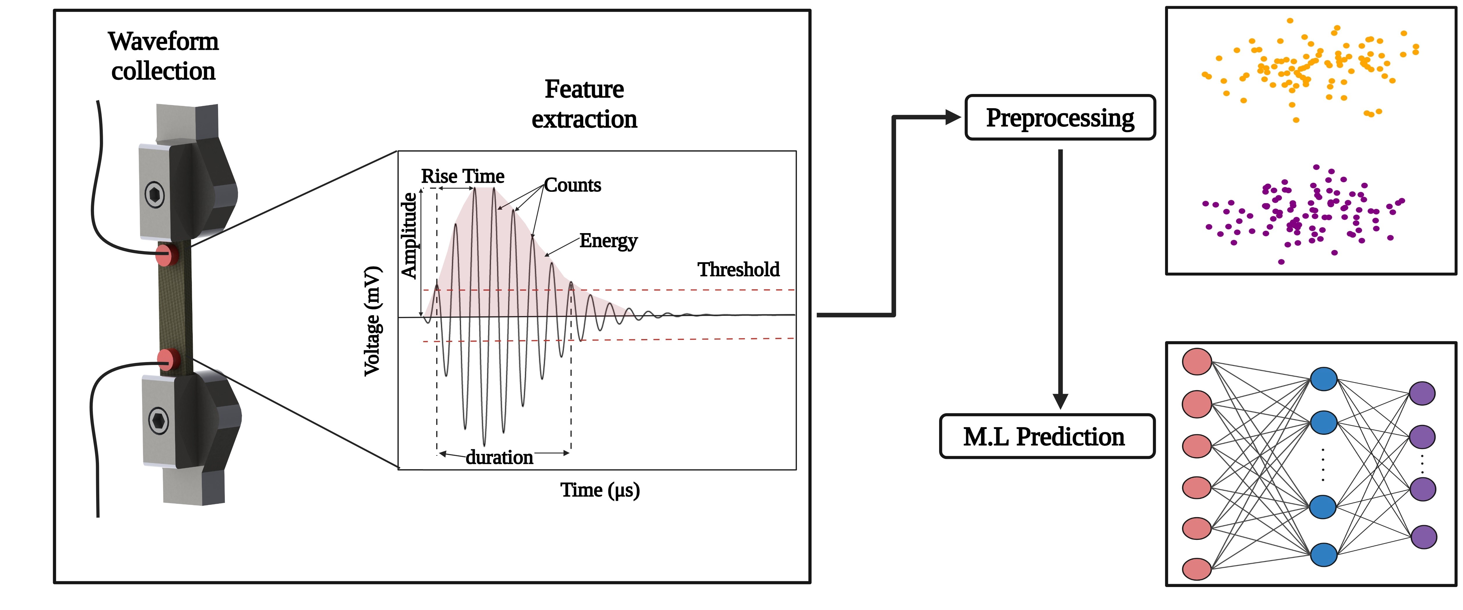
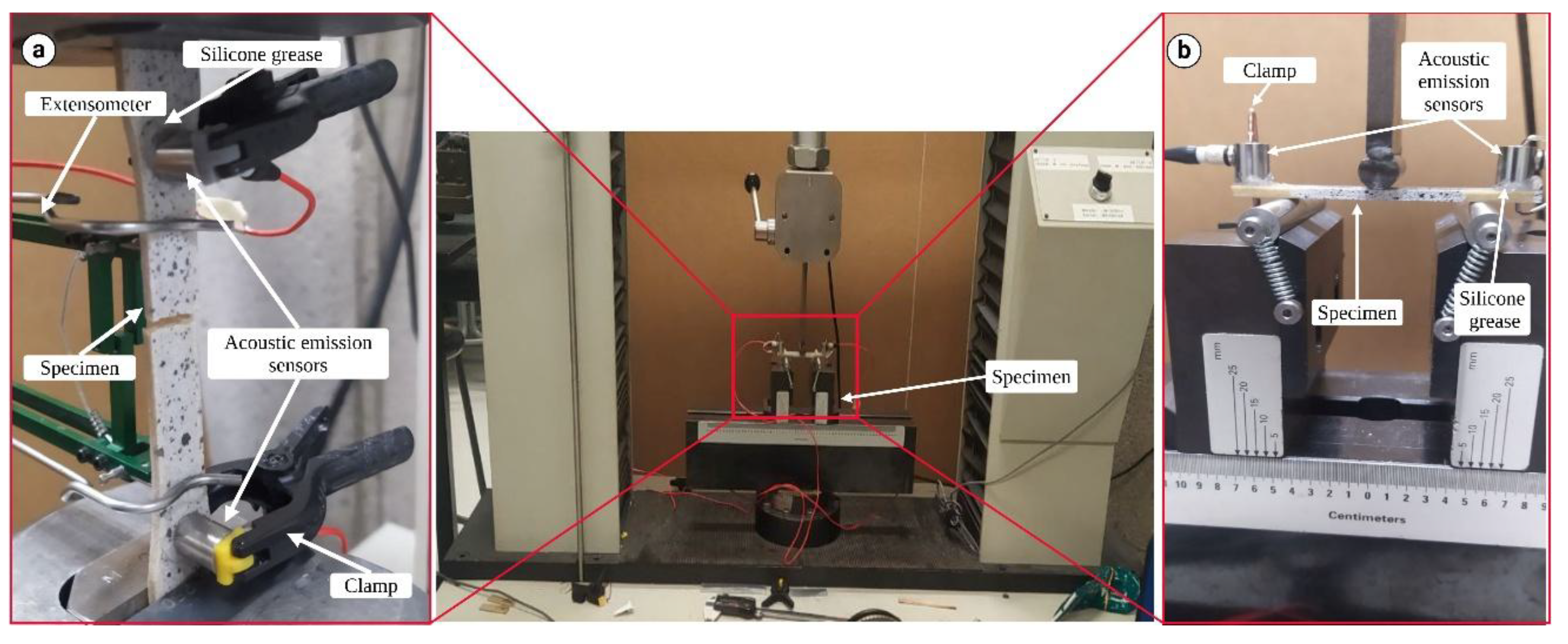
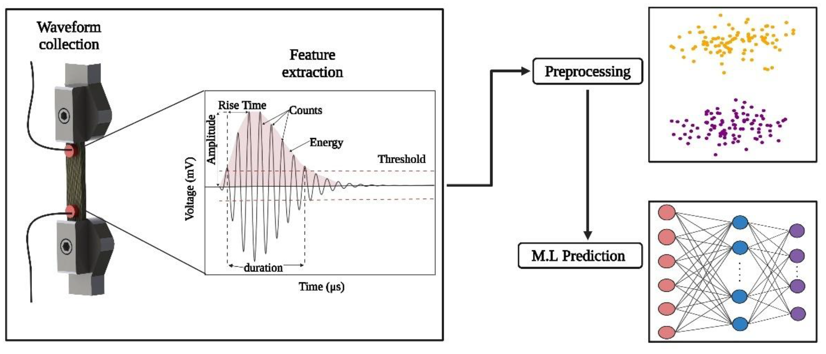
2.2. Mechanical Testing and Acoustic Emission Signal Recording

tensile and Flexion tests were performed on these bio-composite samples to evaluate their mechanical properties (Figure 1). An Instron LM-U150 electromechanical testing equipment with a 50 kN load capacity was used for these tests, which were carried out at room temperature. According to ASTM D638 standard [29], specimens with dimensions of 3.2×13×165 mm (H×W×L) were used for tensile testing. A crosshead speed of 1 mm/min was used, and strain measurements were collected with a 55 mm extensometer. The ASTM D790 [30] standard was followed for performing flexural testing on specimens measuring 3.2×13×80 mm (H×W×L), a crosshead speed of 2.5 mm/min, and a two-point bending arrangement with a 50 mm support span. Each test was repeated four times. Simultaneously, A two-channel physical data acquisition system (MISTRAS, USA) operating at a 4 MHz sampling rate with 40 dB pre-amplification was used for collecting acoustic emission (AE) data. Two resonant MICRO-80 sensors were used to detect AE signals from 100 to 1000 kHz with a 35 dB threshold to eliminate the noise. The steps for preprocessing acoustic emission data and preparing it for machine learning prediction are shown in Figure 2.

2.3. Machine Learning Models

In this study, six input features: cumulative rise, duration, count, frequency, energy, and amplitude from acoustic emission data were utilized to train four machine learning models that predicted stress levels for 3D-printed bio-composite specimens under mechanical testing. Normalization of these features was done to guarantee consistent scaling for all variables. To achieve optimal performance, specific parameters within each model were fine-tuned through hyperparameter optimization (Table 1). Beyond a standard 80/20 train-test split, the training process incorporated rigorous 5-fold cross-validation to assess model generalizability and accuracy. Model performance was evaluated using R-squared and Mean Squared Error (MSE) metrics. These metrics were calculated for each cross-validation fold and the holdout test set (Figure 3).

To get the best results from a model, it’s critical to avoid overfitting and underfitting. Overfitting occurs when a model learns too much from the training data and has difficulty making accurate predictions on new data. This can be prevented by techniques like normalization, early stopping, and hyperparameter tuning [31]. Underfitting occurs when a model doesn’t learn enough from the training data and performs poorly on both training and new data. This can be addressed by increasing training time, optimizing hyperparameters, or using more complex models [32,33].

2.4. Preparation of Acoustic Emission Data

The acoustic emission (AE) data was cleaned to eliminate outliers, mostly generated by undesired noise from mechanical friction, electromechanical components, and ambient noise. These disturbances can affect the frequency content and amplitude of the recorded signals. If not filtered, these disturbances can lead to outliers in the AE data [14,34,35]. The Interquartile Range (IQR) approach was employed for outlier detection in order to increase the accuracy of our predictive models. Extreme values can be acquired with the help of the IQR technique. The dataset utilized for machine learning analysis was made more accurate and representative through this cleaning process.

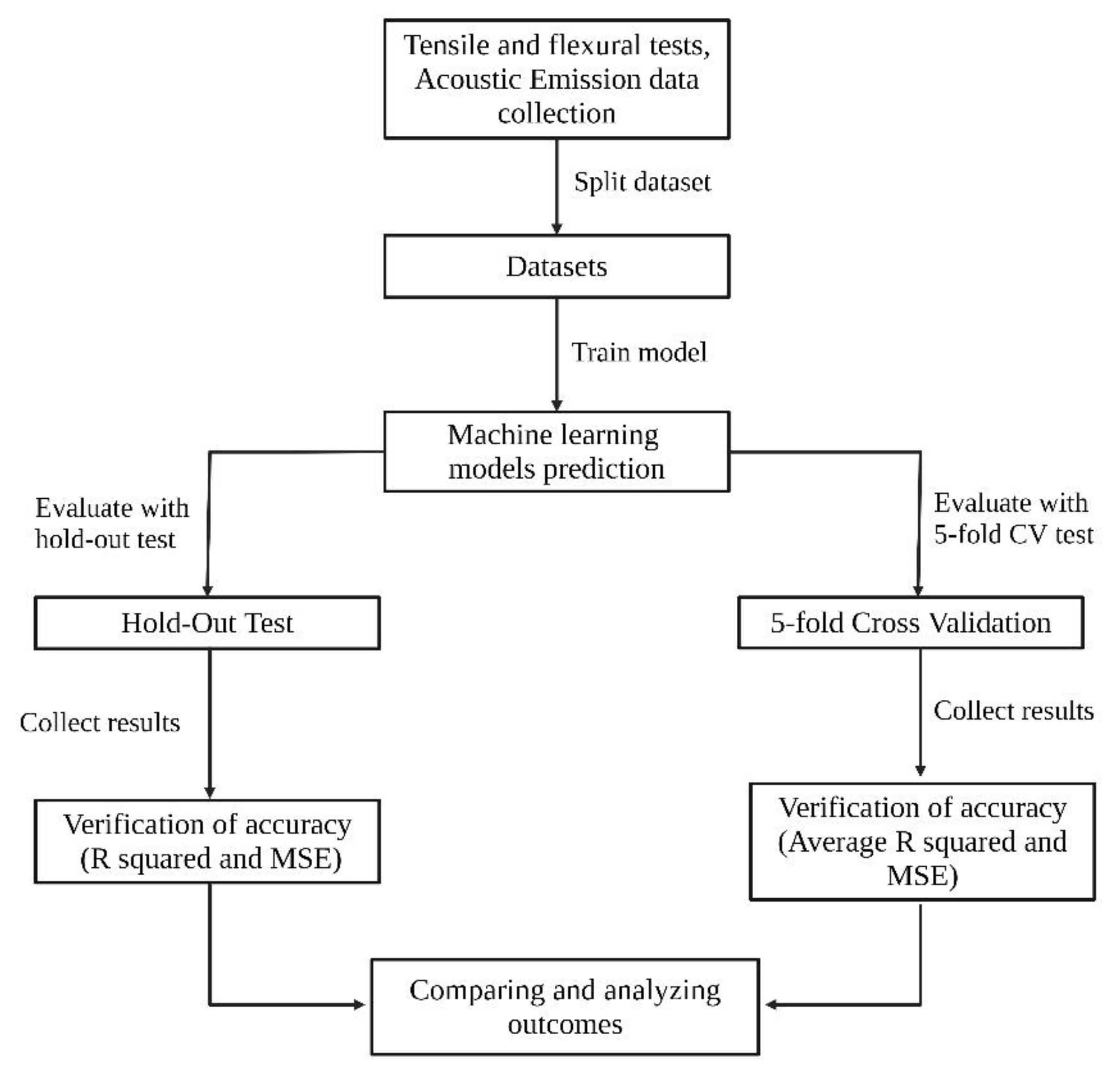
2.5. Cross-Validation and Hold-Out Evaluation

The hold-out method divides the data set into two separate portions, with 80% used for training and the remaining 20% for evaluation. This split offers a simple method to assess how well a model replies to new untested data.

Based on the hold-out method, cross-validation offers a more dependable statistical technique for adjusting hyperparameters. One of the commonly used Cross-validation techniques is the 5-fold CV. Using this process, the dataset was divided into five equal portions. In each iteration of the process, the model is trained in four splits, with the remaining parts utilized for validation. During the course of this cycle’s five repetitions, each of the five components acts as the validation set precisely once. This ensures that every data point was utilized exactly once for both training and validation, enabling a full investigation of the model’s performance throughout the whole data set [36].

2.6. Verification of Accuracy

Metrics like mean squared error (MSE) and coefficient of determination (R²) are frequently used to assess the performance of models. These metrics offer a thorough understanding of the model’s performance when paired with predicted and actual values plots [37]. Whereas MSE measures the average squared difference between predicted and observed values and provides information about the model’s prediction accuracy, R² indicates the proportion of the dataset’s variance that the model successfully explains. The calculation of R² and MSE is outlined as follows:

$${\mathrm{R}}^2=1-{\displaystyle \frac{\sum _{\mathrm{i}=1}^{\mathrm{n}}{\left({\mathrm{y}}_{\mathrm{i}-}{\widehat{\mathrm{y}}}_{\mathrm{i}}\right)}^2}{\sum _{\mathrm{i}=1}^{\mathrm{n}}{\left({\mathrm{y}}_{\mathrm{i}-}\overline{\mathrm{y}}\right)}^2}}$$

Where $y_i$ denotes the actual observed values from the dataset, while ${\widehat{y}}_i$ represents the estimated values generated by the regression model. Additionally, $\overline{y}$refers to the mean of the actual data.

$$MSE={\displaystyle \frac{1}{n}}\sum _{n=1}^n{\left(y_i-{\mathrm{ŷ}}_i\right)}^2$$

Where n refers to the total number of observations, $y_i$represents the actual values, and ${\widehat{y}}_i$ is the estimated values by the model.

2.7. Damage Mode Identification Using K-Means Clustering Algorithm

The k-means clustering algorithm is a cornerstone in data analysis, praised for its simplicity and efficacy in determining cluster centers that reflect distinct regions within a dataset. It executes through an iterative two-step process: first, Each data point is allocated to the closest cluster center, after which every center of the cluster is recalculated as the mean of the data point assigned to it, as noted by [38]. This assignment is reiterated until no data points remain unassigned. Following this, the centroid positions are refined iteratively until the objective function, JJ, which is defined as:

$$J=\sum _{j=1}^k\sum _{i=1}^n‖x_i^{\left(i\right)}-c_i^2‖$$

where $‖x_i^{\left(i\right)}-c_i^2‖$measures the squared Euclidean distance between each point $x_i^{\left(i\right)}$ and its cluster center . This distance indicates how close each n-th data point is to its cluster center. The operation is repeated until the centroids stabilize, thereby segregating the data into distinct classes that minimize intra-cluster distances [39].

In this study, the k-means algorithm (unsupervised machine learning model) was employed to classify acoustic emission (AE) data into predefined categories based on the AE data recorded during mechanical tests. The number of clusters was determined with insights from scanning electron microscopy (SEM) analysis, linking the count of damage modes directly to the microstructural damage observed in SEM images. This method effectively identified distinct damage modes in the biocomposite materials being tested, categorizing the AE data into three main clusters that correspond to variations in AE parameters.

3. Results and Discussion

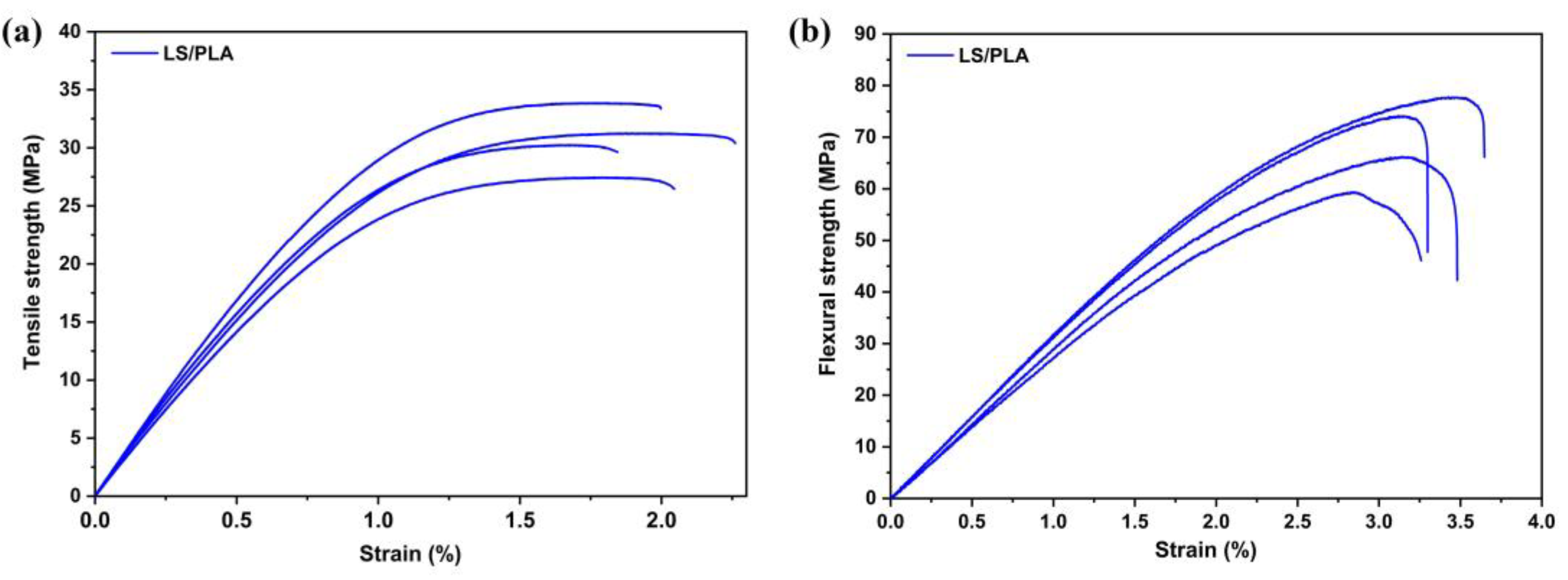
3.1. Mechanical Properties

Eight specimens of the Lygeum spartum/PLA biocomposite were tested for their mechanical properties using tensile and flexural tests. The results were illustrated in a stress-strain curve Figure 4, which represents the relationship between the applied stress and the deformation of the material.

The specimens have a stress range of 27.45-33.85 MPa, showing the LS/PLA biocomposite’s mechanical characteristics under tensile stress. The strain range is reported at 1.84-2.27%, demonstrating the material’s capacity to deform before failure. The composite’s

tensile modulus is in average of 3.24 GPa, demonstrating a stable stiffness in the material. These features indicate LS fibers’ contribution to the overall mechanical behavior, demonstrating the biocomposite’s promise for applications that need both strength and flexibility.

for the flexural testing the LS/PLA specimens exhibit a stress range of 64.67-88.76 MPa, with an average value of 75.69 MPa, demonstrating a good strength characteristic. Additionally, these specimens show a strain range of 2.79-3.74% with an average value of 3.31%.

The results indicate an acceptable mechanical properties of the LS/PLA biocomposites, owing to the effective adhesion between the layers and the absence of gaps and voids within the layers. This have been confirmed by SEM images of the cross-sections of the specimens after fracture in , showing a coherent and gap-free structure. Such structural integrity in the composite specimens minimizes delamination and enhances material strength, as noted in the literature [40].

3.2. Analysis of Damage Using Acoustic Emission

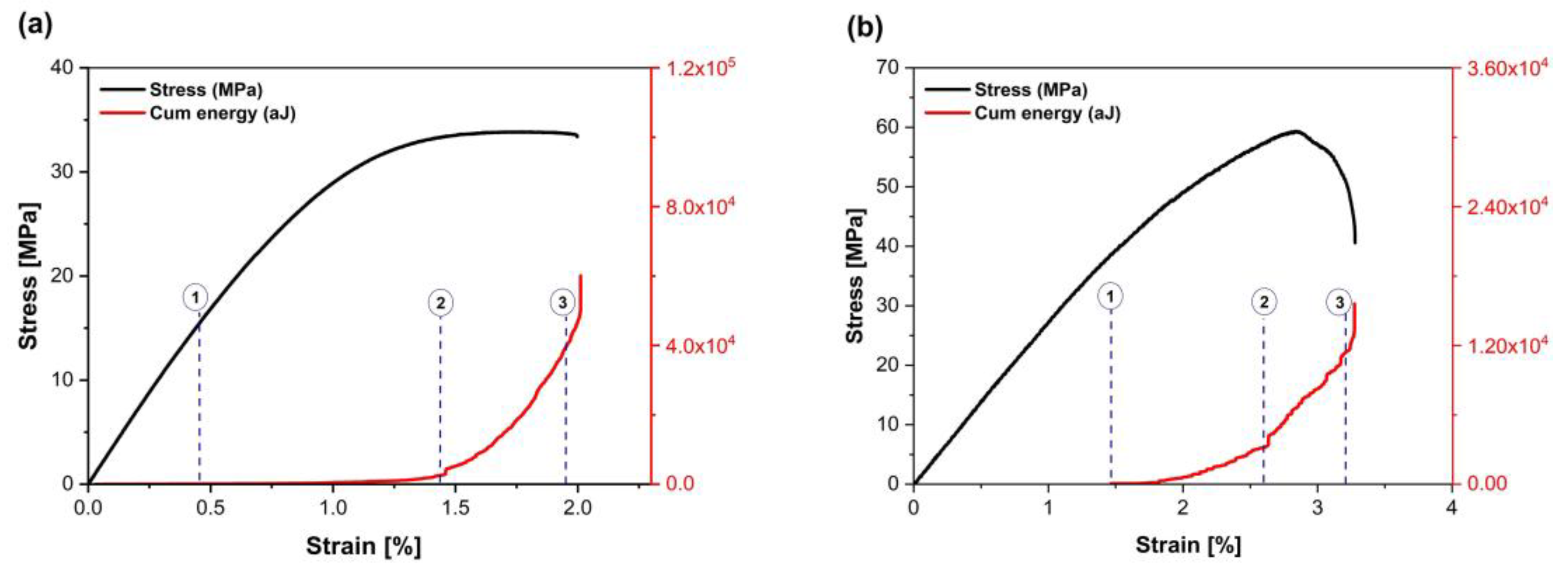
3.2.1. Damage Evolution

Figure 5 illustrates the curves of stress-strain for LS/PLA composite along with the corresponding AE energy accumulations for both types of tests. For the tensile and flexural tests, the evolution of the acoustic emission (AE) energy shows four distinct phases. In the first phase, before position 1 in Figure 5, corresponds to the elastic phase of the deformation curve, where no AE signal is recorded above the noise threshold. The detection of the first significant AE signal marks the beginning of the second phase (zone 1–2). This signal range is related to a specific failure mode in composites, such as matrix cracking. This stage is distinguished by a very low AE activity. At the end of this phase, significant AE activity is observed (point 2). From this point, the AE energy increases exponentially (zone 2-3), indicating an acceleration of damage and the appearance of new failure mechanisms, such as decohesion or fiber-matrix friction. The fourth phase, occurring after point 3, is marked by a sudden increase in energy immediately preceding the final failure.

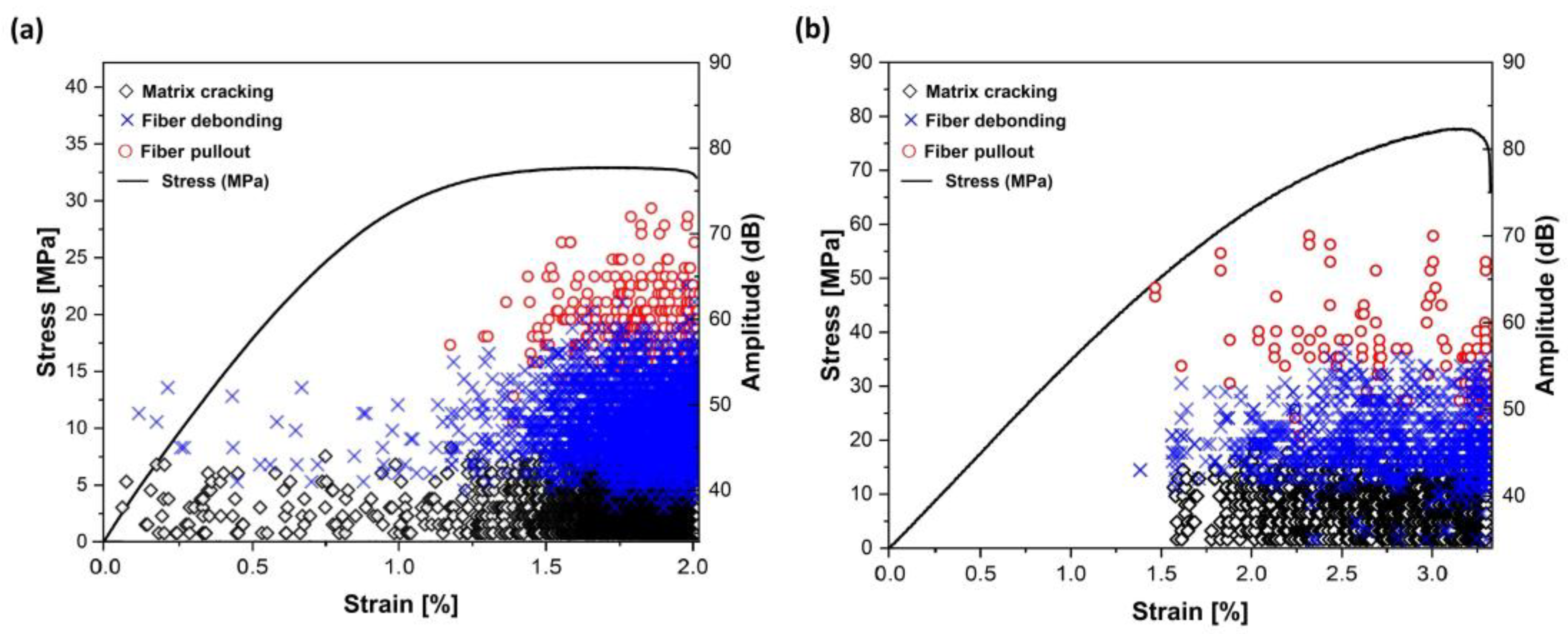
3.2.2. Classification of the Damage Modes Using K-Means Clustering

The changes in mechanical behavior are often linked to variations in failure modes. The accumulated energy of acoustic emission bursts provides an idea of the evolution of this behavior (elastic, plastic phases, etc.). However, more in-depth information can be obtained by applying, for example, a k-means clustering algorithm, which uses the distinct characteristics of AE signals from localized events to track the evolution of various failure mechanisms during testing. The results presented in Figure 6 for tensile and flexural tests are consistent with existing literature on thermoplastic composites reinforced with natural fibers, indicating an amplitude range of 35-45 dB for matrix cracking, 40-55 dB for fiber debonding, and 50-70 dB for fiber pull-out. The association of failure modes with specific amplitude ranges stems from the results of the clustering algorithm. The clusters reveal that these events can occur simultaneously, but with different intensities.

Scanning electron microscopy (SEM) was used to investigate the fracture facies and confirm the results of the AE analysis. Figure 7 illustrates the fracture facies of specimens subjected to tensile testing. Overall, the mechanisms identified by the AE analysis are observable.

3.3. Prediction of Stress Levels in Tensile and Flexural Tests Using Machine Learning Models

3.3.1. Artificial Neural Network ANN

Based on cumulative Acoustic Emission (AE) features, this work investigates the use of an ANN model to predict the stress levels of 3D-printed bio-composite specimens during tensile and flexural testing. In order to enhance the ANN model, crucial steps were taken, such as choosing relevant AE parameters and eliminating outliers. The model’s structure and the number of layers or nodes was balanced to avoid underfitting and overfitting [41].

The results, illustrated in , show that the ANN model provide a more accurate prediction for tensile stress (R² = 0.9757, MSE = 0.0189) compared to flexural stress (R² = 0.9681, MSE = 0.6490), indicating a nearly perfect correlation for tensile predictions. This discrepancy in predictive accuracy is attributed to the different mechanical responses of bio-composite under tensile and flexural loads, with tensile tests providing richer AE data due to widespread matrix cracking and other failure mechanisms [42,43].

5-fold cross-validation confirmed the model’s reliability, yielding average R² values of 0.9727 for tensile tests and 0.9575 for flexural tests (Table 2). The study concludes that the diversity and richness of AE data are essential for accurately predicting stress levels, as demonstrated by the superior performance in tensile testing. In contrast, flexural testing predominantly engages the material in the central region where stress is maximized, confining the occurrence of these mechanisms to a localized zone [44]. These results in a more constrained AE signature, potentially limiting the model’s exposure to the full range of signal patterns associated with the material’s failure modes.

3.3.2. Random Forest Regression RFR

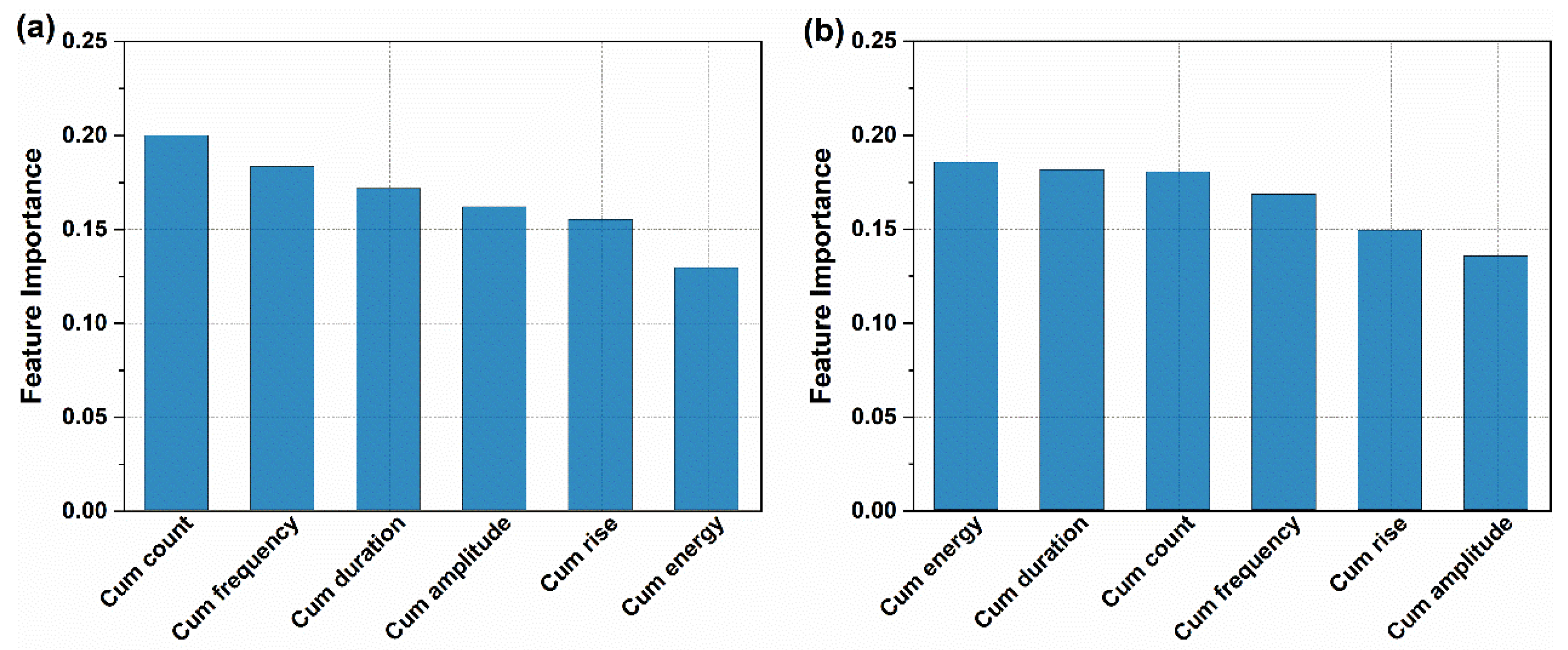
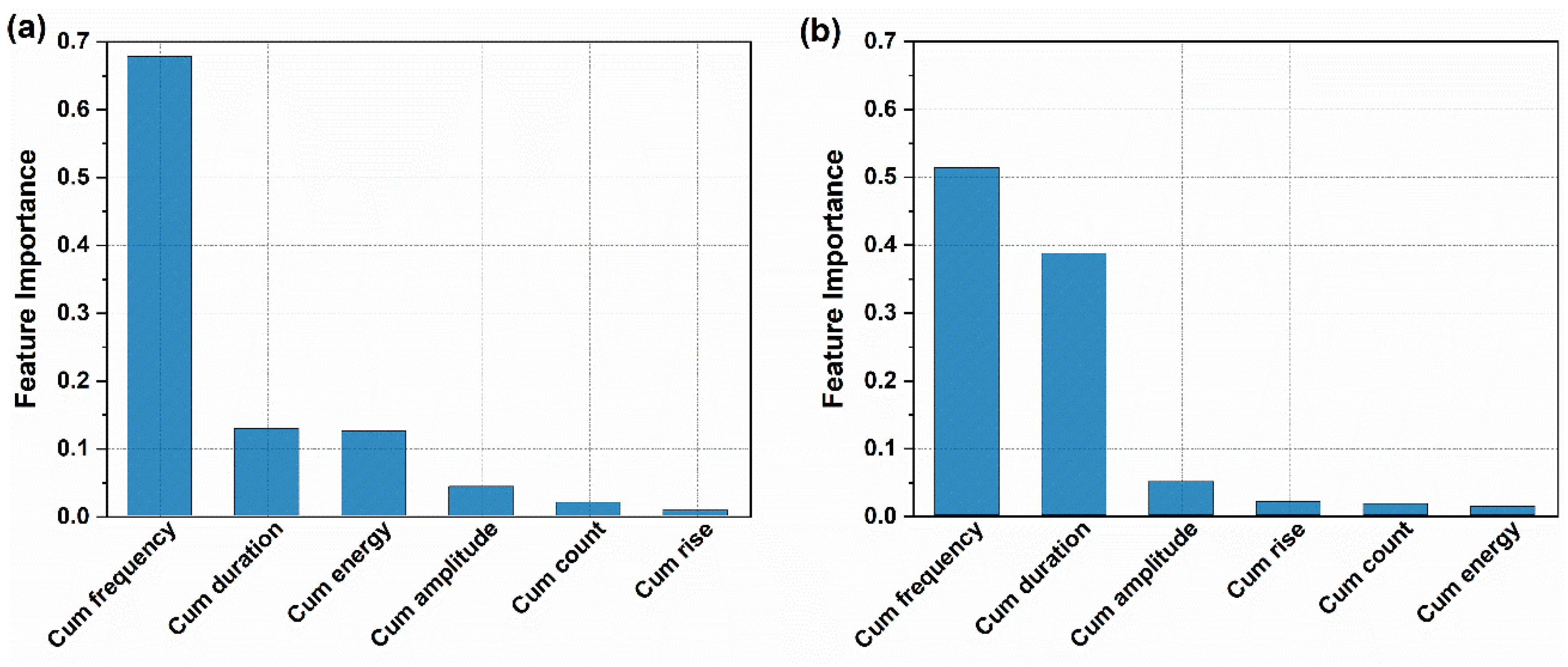
3.3.2.1. Feature Importance Analysis

The feature importance analysis within the RFR model highlighted key Acoustic Emission (AE) signal features correlated with predicted stress levels. Similar to the studies by Shimamoto, Yuma, et al.[26] and Lee, Hang-Lo, et al.[45] , the cumulative AE for each feature were used as inputs. The analysis in Figure 8 revealed that cumulative count was the most significant predictor for tensile test, followed by cumulative frequency and duration. Cumulative amplitude, energy, and rise had lesser effects but still contributed nearly equally. For the flexural test, cumulative energy emerged as the most significant predictor, followed by cumulative duration, cumulative count, and cumulative frequency. Cumulative rise and amplitude had the least impact on the model. These findings improve the model and provide a thorough knowledge of the relation between mechanical properties and AE signals.

3.3.2.2. Stress Level Prediction Using RFR

The scatter plot in compares predicted to actual stress levels and shows the prediction results for the RFR model. The model demonstrates strong predictive capabilities in predicting the stress levels of this material under both tensile and flexural testing. With an R² of 0.9822 and MSE of 0.013 for the tensile test. Similarly, the flexural test shows a significant correlation accuracy with an R² of 0.9813 and an MSE of 0.3792.

The 5-fold cross-validation further validates the results, with an average R² of 0.9801 for tensile testing and 0.9806 for flexural testing (Table 2), demonstrating the model’s stability and consistency in performance across various data subsets.

3.3.3. Decision Tree Regression DTR

3.3.3.1. Feature Importance

Feature importance in DTR model is determined by the extent to which each feature reduces impurity at each split, with greater reductions indicating higher relevance. However, this importance can be less stable than in RFR, as it relies on a single tree sensitive to the training data. Figure 9 shows that cumulative frequency is the most important feature compared to the others.

3.3.3.2. Stress Level Prediction Using DTR

The predicted stress levels estimated by the DT model are illustrated in the scatter plot in Figure 10 and Figure 11. The model demonstrates a high predictive capability, With an R² score of 0.9652 and an MSE of 0.0271 for the tensile test, and an R² of 0.9681 and an MSE of 0.6480 for the flexural test. For the 5-fold cross-validation, the model produces consistent results comparable to the holdout test (Table 2). These metrics indicate that the model has solid predictive capabilities for both tests.

By examining the feature importance results from the DT model (Figure 9), the significant differences observed suggest that the model can produce reasonable results by using only the most important features. Specifically, cumulative frequency in the tensile test, and cumulative frequency, cumulative duration, and amplitude in the flexural test, appear as key inputs.

3.3.4. Support Vector Regression SVR

SVR is one of the ML designed for tasks of regression processes. Unlike typical regression models, the SVR aims to find the hyperplane optimally fits the data within a preset margin of error. It works by minimize the error while maximizing the margin, allowing some errors or deviations within a certain threshold (epsilon). the SVR method is especially beneficial for high dimensional data because it may capture complicated connections using kernel functions. These functions convert the used data into a higher dimensional space, and make it easier to find linear relationships that might not be evident in the original space [46].

The estimated stress levels predicted by this model are displayed in the Figure 10 and Figure 11. For the tensile test, the model gives an R² value of 0.9442 and an MSE of 0.0435, while for the flexural test, it attained an R² of 0.9683 and an MSE of 0.4411.

The model also achieved in the 5-fold cross-validation an R² values of 0.9526 for tensile testing and 0.9671 for flexural testing, demonstrating stable predictive capabilities across all datasets (Table 2).

3.4. Comparative Performance Analysis of the Employed ML Models

Table 2 presents a comparative analysis of the performance of various machine learning (ML) models. The ANN had challenges with flexural testing, as proven by its MSE and R² values. Meanwhile, the RFR model, an ensemble technique that leverages the voting mechanism among multiple decision trees, emerged as the most accurate and consistent predictor compared to the rest models. The DT and SVR models, though useful, performed slightly less effectively in both tests, demonstrating limitations in handling the complexity of the dataset.

The higher MSE and RMSE values observed in all ML models for the flexural test can be attributed to the smaller dataset relative to the tensile test. Furthermore, the maximum stress in the flexural test exceeds 60 MPa, whereas the tensile test stress remains below 32 MPa. This disparity likely contributes to the consistently elevated MSE and RMSE values in predicting flexural stress as compared to tensile stress.

Despite minor differences in performance, all models exhibited strong predictive capabilities, with the lowest R² value exceeding 0.94, reflecting high accuracy. This impressive outcome can be attributed to the stability and richness of the data, along with meticulous data preparation. Key factors like effective outlier removal and carefully tuned hyperparameters significantly enhanced the models’ ability to capture the complex relationships within the dataset. Additionally, the thorough approach to data preparation and model training ensured that each model was well-equipped to address the intricacies of both tensile and flexural testing, providing reliable insights into material behavior.

4. Conclusions

This research investigates the damage evolution and the use of four machine learning models for the prediction of the stress levels in a bio-composite composed of a PLA matrix reinforced with Lygeum Spartum fiber, utilizing acoustic emission data. The main conclusions are outlined below:

• Cumulative Acoustic Emission Data: The cumulative acoustic emission energy provides critical insights into the damage evolution within the material during mechanical testing, serving as valuable indicators of structural integrity.
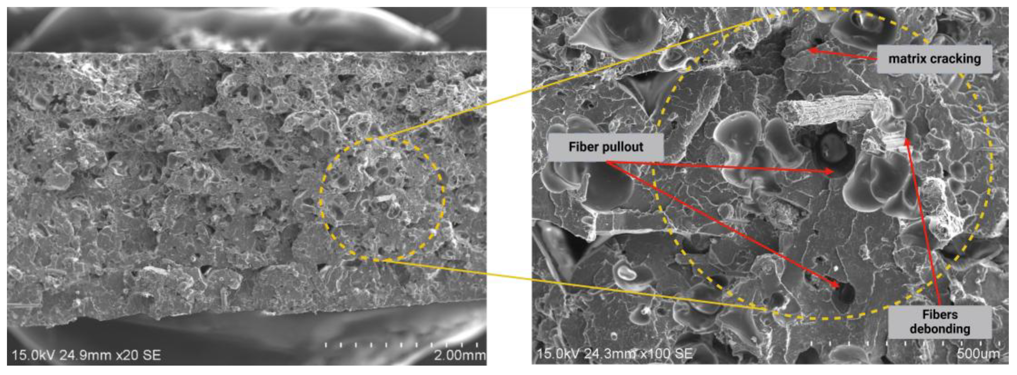
• The K-means model is used to classify damage modes, resulting in the identification of three main modes: matrix cracking, fiber debonding and pull-out.
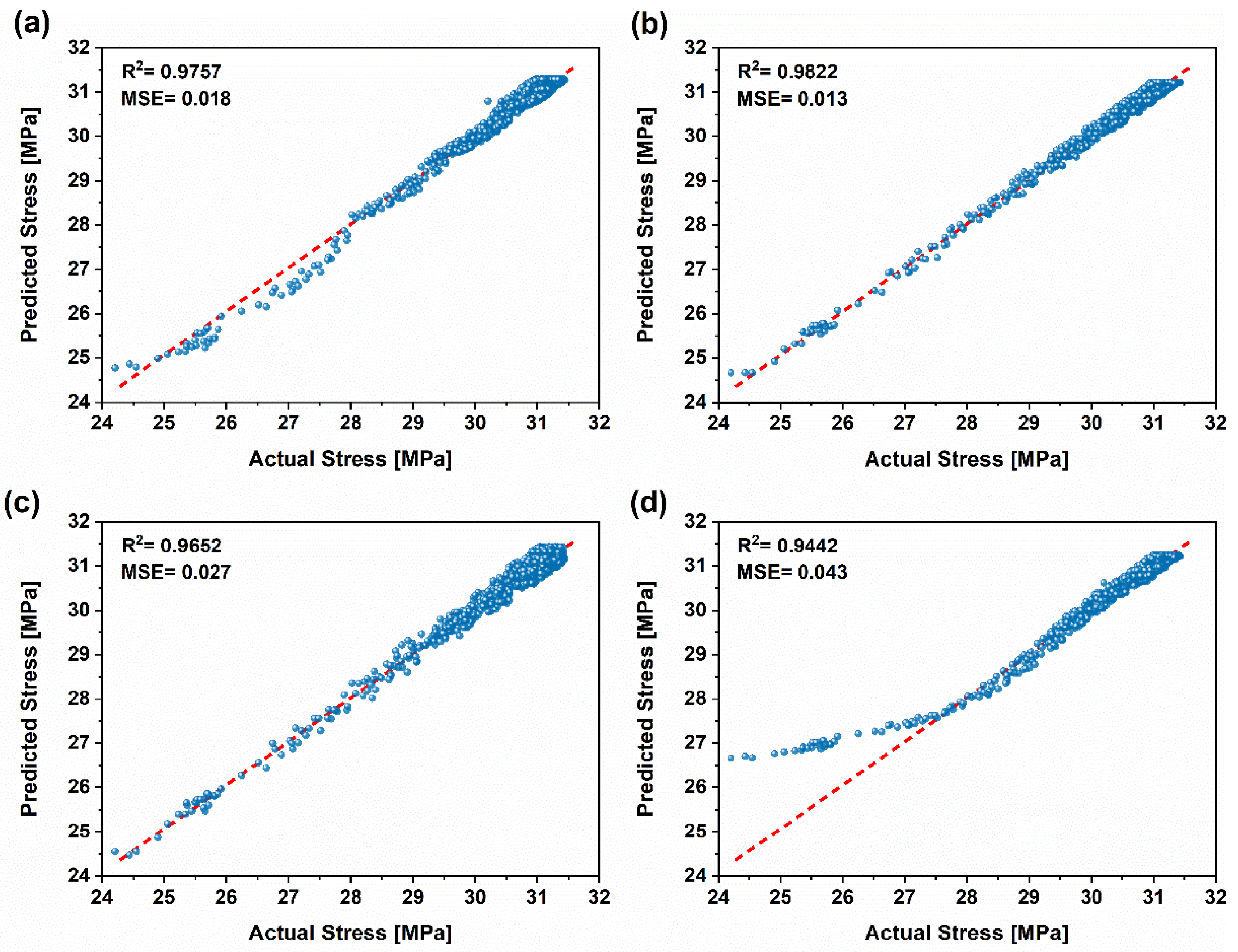
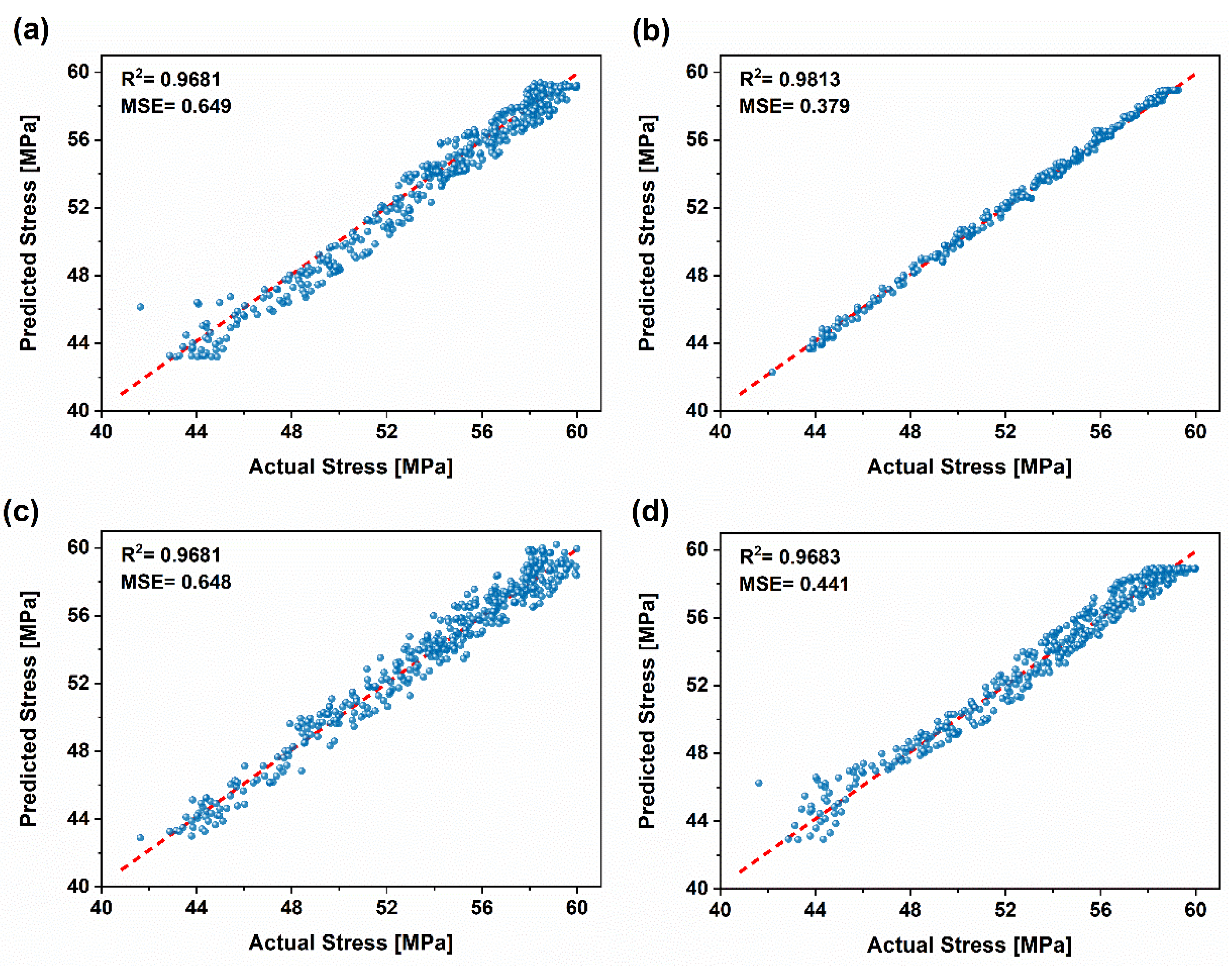
• Machine Learning Model Performance: Four machine learning models with tuned hyperparameters were employed to estimate stress levels during tensile and flexural testing, using cumulative acoustic emission parameters. Among these, the RFR model delivered the most accurate predictions, outperforming the other models, followed by ANN, DTR, and SVR.
• Data Richness and Prediction Accuracy: The richness of the acoustic emission data contributed to superior predictive capabilities, particularly in the tensile test, as compared to the flexural test.

In conclusion, the integration of acoustic emission data with multiple machine learning models has proven to be an effective approach for health monitoring of bio-composite materials. This research advances the field of materials science by demonstrating the potential of these techniques to enhance of prediction accuracy and understanding of bio-composite behavior under stress.

References

1. Ayrilmis, N., et al., Effect of printing layer thickness on water absorption and mechanical properties of 3D-printed wood/PLA composite materials. The International Journal of Advanced Manufacturing Technology, 2019. 102: p. 2195-2200. [CrossRef]
2. Bahrami, M. Abenojar, and M.Á. Martínez, Recent progress in hybrid biocomposites: Mechanical properties, water absorption, and flame retardancy. Materials, 2020. 13(22): p. 5145. [CrossRef]
3. Trivedi, A.K. Gupta, and H. Singh, PLA based biocomposites for sustainable products: A review. Advanced Industrial and Engineering Polymer Research, 2023. 6(4): p. 382-395. [CrossRef]
4. Le Duigou, A., et al., 3D printing of wood fibre biocomposites: From mechanical to actuation functionality. Materials & Design, 2016. 96: p. 106-114. [CrossRef]
5. Bianchi, I., et al., Comparison between the mechanical properties and environmental impacts of 3D printed synthetic and bio-based composites. Procedia CIRP, 2022. 105: p. 380-385. [CrossRef]
6. Tao, Y., et al., Development and application of wood flour-filled polylactic acid composite filament for 3D printing. Materials, 2017. 10(4): p. 339. 339, 2017. [CrossRef]
7. Guo, R., et al., Effect of toughening agents on the properties of poplar wood flour/poly (lactic acid) composites fabricated with Fused Deposition Modeling. European Polymer Journal, 2018. 107: p. 34-45. [CrossRef]
8. Panasiuk, K. and K. Dudzik, Determining the stages of deformation and destruction of composite materials in a static tensile test by acoustic emission. Materials, 2022. 15(1): p. 313. [CrossRef]
9. Barile, C., et al., Damage monitoring of carbon fibre reinforced polymer composites using acoustic emission technique and deep learning. Composite Structures, 2022. 292: p. 115629. [CrossRef]
10. Huijer, A. Kassapoglou, and L. Pahlavan, Acoustic emission monitoring of carbon fibre reinforced composites with embedded sensors for in-situ damage identification. Sensors, 2021. 21(20): p. 6926. [CrossRef]
11. Karami, S., et al., Investigation of the effect of nanoparticles on wood-bioplastic composite behavior using the acoustic emission method. Journal of Composite Materials, 2023. 57(1): p. 23-34. [CrossRef]
12. Salje, E.K., et al., Acoustic emission spectroscopy: Applications in geomaterials and related materials. Applied Sciences, 2021. 11(19): p. 8801. [CrossRef]
13. Hao, W., et al., Acoustic emission characterization of tensile damage in 3D braiding composite shafts. Polymer Testing, 2020. 81: p. 106176. [CrossRef]
14. Ciaburro, G. and G. Iannace, Machine-learning-based methods for acoustic emission testing: A review. Applied Sciences, 2022. 12(20): p. 10476. [CrossRef]
15. Habibi, M., et al., Combining short flax fiber mats and unidirectional flax yarns for composite applications: Effect of short flax fibers on biaxial mechanical properties and damage behaviour. Composites Part B: Engineering, 2017. 123: p. 165-178. [CrossRef]
16. Saidane, E.H., et al., Damage mechanisms assessment of hybrid flax-glass fibre composites using acoustic emission. Composite Structures, 2017. 174: p. 1-11. [CrossRef]
17. Sobhani, A., et al., The study of buckling and post-buckling behavior of laminated composites consisting multiple delaminations using acoustic emission. Thin-Walled Structures, 2018. 127: p. 145-156. 2018. [CrossRef]
18. Malpot, A. Touchard, and S. Bergamo, An investigation of the influence of moisture on fatigue damage mechanisms in a woven glass-fibre-reinforced PA66 composite using acoustic emission and infrared thermography. Composites Part B: Engineering, 2017. 130: p. 11-20. [CrossRef]
19. Roundi, W., et al., Acoustic emission monitoring of damage progression in glass/epoxy composites during static and fatigue tensile tests. Applied Acoustics, 2018. 132: p. 124-134. [CrossRef]
20. Saeedifar, M. and D. Zarouchas, Damage characterization of laminated composites using acoustic emission: A review. Composites Part B: Engineering, 2020. 195: p. 108039. [CrossRef]
21. Xu, D. Liu, and Z. Chen, A deep learning method for damage prognostics of fiber-reinforced composite laminates using acoustic emission. Engineering Fracture Mechanics, 2022. 259: p. 108139. [CrossRef]
22. König, F., et al., Machine learning based anomaly detection and classification of acoustic emission events for wear monitoring in sliding bearing systems. Tribology International, 2021. 155: p. 106811. [CrossRef]
23. Zhou, W., Y. Zhang, and W. Zhao. Tensile Deformation Damage and Clustering Analysis of Acoustic Emission Signals in Three-Dimensional Woven Composites. in Advances in Acoustic Emission Technology: Proceedings of the World Conference on Acoustic Emission-2017. 2019. Springer. [CrossRef]
24. Lu, D. and W. Yu, Predicting the tensile strength of single wool fibers using artificial neural network and multiple linear regression models based on acoustic emission. Textile Research Journal, 2021. 91(5-6): p. 533-542. [CrossRef]
25. Sause, M.G. Schmitt, and S. Kalafat, Failure load prediction for fiber-reinforced composites based on acoustic emission. Composites Science and Technology, 2018. 164: p. 24-33. [CrossRef]
26. SHIMAMOTO, Y., et al., Estimation of Concrete Mechanical Properties by Acoustic Emission with Random Forest Algorithm. [CrossRef]
27. Wang, Z., et al., Acoustic emission characterization of natural fiber reinforced plastic composite machining using a random forest machine learning model. Journal of Manufacturing Science and Engineering, 2020. 142(3): p. 031003. [CrossRef]
28. Ai, L., et al., Acoustic Emission-Based Detection of Impacts on Thermoplastic Aircraft Control Surfaces: A Preliminary Study. Applied Sciences, 2023. 13(11): p. 6573. [CrossRef]
29. Properties, A.S.D.o.M. Standard Test Method for Tensile Properties of Plastics. 1998. American Society for Testing and Materials.
30. Standard, A., Standard test methods for flexural properties of unreinforced and reinforced plastics and electrical insulating materials. ASTM D790. Annual book of ASTM standards, 1997.
31. Ying, X. An overview of overfitting and its solutions. in Journal of physics: Conference series. 2019. IOP Publishing. 022022. [CrossRef]
32. Bashir, D., et al. An information-theoretic perspective on overfitting and underfitting. in AI 2020: Advances in Artificial Intelligence: 33rd Australasian Joint Conference, AI 2020, Canberra, ACT, Australia, November 29–30, 2020, Proceedings 33. 2020. Springer. [CrossRef]
33. Pothuganti, S., Review on over-fitting and under-fitting problems in Machine Learning and solutions. Int. J. Adv. Res. Electr. Electron. Instrum. Eng, 2018. 7: p. 3692-3695. [CrossRef]
34. Barsoum, F.F., et al., ACOUSTIC EMISSION MONITORING AND FATIGUE LIFE PREDICTION IN AXIALLY LOADED NOTCHED STEEL SPECIMENS. 2009. 27.
35. Benabderazag, K., et al., Characterization of thermomechanical properties and damage mechanisms using acoustic emission of Lygeum spartum PLA 3D-printed biocomposite with fused deposition modelling. 2024. 186: p. 108426. [CrossRef]
36. Xiong, Z., et al., Evaluating explorative prediction power of machine learning algorithms for materials discovery using k-fold forward cross-validation. Computational Materials Science, 2020. 171: p. 109203. [CrossRef]
37. Beyeler, M., Machine Learning for OpenCV. 2017: Packt Publishing Ltd. [CrossRef]
38. Müller, A.C. and S. Guido, Introduction to machine learning with Python: a guide for data scientists. 2016: “ O’Reilly Media, Inc.”.
39. Kaufman, L. and P.J. Rousseeuw, Finding groups in data: an introduction to cluster analysis. 2009: John Wiley & Sons.
40. Djabali, A., et al., Fatigue damage evolution in thick composite laminates: Combination of X-ray tomography, acoustic emission and digital image correlation. Composites Science and Technology, 2019. 183: p. 107815. [CrossRef]
41. Karsoliya, S., Approximating number of hidden layer neurons in multiple hidden layer BPNN architecture. International Journal of Engineering Trends and Technology, 2012. 3(6): p. 714-717.
42. Li, P., et al., Analysis of acoustic emission energy from reinforced concrete sewage pipeline under full-scale loading test. Applied Sciences, 2022. 12(17): p. 8624. [CrossRef]
43. Karthik, M. and C.S. Kumar, A comprehensive review on damage characterization in polymer composite laminates using acoustic emission monitoring. Russian Journal of Nondestructive Testing, 2022. 58(8): p. 705-721. [CrossRef]
44. Han, S.N.M.F., et al., Investigation of tensile and flexural properties of kenaf fiber-reinforced acrylonitrile butadiene styrene composites fabricated by fused deposition modeling. Journal of Engineering and Applied Science, 2022. 69(1): p. 52. [CrossRef]
45. Lee, H.-L., et al., Ensemble learning approach for the prediction of quantitative rock damage using various acoustic emission parameters. Applied Sciences, 2021. 11(9): p. 4008. [CrossRef]
46. Koya, B.P., et al., Comparative analysis of different machine learning algorithms to predict mechanical properties of concrete. Mechanics of Advanced Materials and Structures, 2022. 29(25): p. 4032-4043. [CrossRef]
Figure 1. LS/PLA Bio-composite specimens produced through 3D printing and the acoustic emission setup for tensile test (a) and flexural test (b).
Preprints 147507 g001
Figure 2. Experimental procedure for recording acoustic emissions and preparing the data for machine learning prediction.
Preprints 147507 g002
Figure 3. Machine learning prediction methodology.
Preprints 147507 g003
Figure 4. Typical stress–strain curves for the LS/PLA biocomposite specimens, (a) tensile test and (b) flexural test.
Preprints 147507 g004
Figure 5. stress-strain curves, as well as the cumulative acoustic emission energy, for the composite during tensile (a) and flexural testing (b).
Preprints 147507 g005
Figure 6. stress–strain curves with corresponding AE amplitudes classified with k-means algorithm.
Preprints 147507 g006
Figure 7. Fracture surface of the specimen after mechanical testing, highlighting the observed damage mechanisms.
Preprints 147507 g007
Figure 8. Feature importance contributing to the predictions of the RFR model for tensile test (a), and flexural test (b).
Preprints 147507 g008
Figure 9. Feature importance in DT: (a) tensile test and (b) flexural test.
Preprints 147507 g009
Figure 10. Stress levels estimated for tensile testing using ML models: (a) ANN, (b) RFR, (c) DTR, and (d) SVR.
Preprints 147507 g010
Figure 11. Stress levels estimated for flexural testing using machine learning models: (a) ANN, (b) RFR, (c) DTR, and (d) SVR.
Preprints 147507 g011