
Submitted:
27 January 2025
Posted:
28 January 2025
You are already at the latest version
Abstract
After the detection of the gravitational wave GW170817 from a binary neutron star merger and the simultaneous detection of the electromagnetic signals, multi-messenger astronomy enters a new era. Furthermore, the GRBs (Gamma-Ray Bursts) and the mysterious FRBs (Fast Radio Bursts) have sparked interest in the development of new detectors and telescopes dedicated to the time-domain astronomy across all the electromagnetic spectrum. Fast Infra-red Bursts (FIRBs) have been relatively understudied, often due to the lack of appropriate tools for observation and analysis. In this scenario, the present contribution proposes a new detection system for mid-infrared ground-based telescopes. Experience developed in the diagnostics for lepton circular accelerators has been used to design temporal devices for astronomy. At SINBAD, the infrared beam line of DAFNE, the detector has acquired fast infrared pulses with 2-12 µm wavelengths and 1 ns rise times with sensitivity up to 1 photon implementing the proper amplification. A dedicated data acquisition system has been designed, including simulations for smart triggers and AI pattern recognition techniques. The classification of the most interesting transient candidates found is performed by implementing an off-line fast instability analysis derived from accelerator physics techniques. This contribution aims to be a step toward a feasibility study report.
Keywords:
multi-messenger astronomy
; time-domain astronomy
; fast infrared bursts
; fast transients
; HgCdTe detectors
; infrared time-resolved detector
; infrared telescopes
; pattern recognition
1. Introduction
The main motivation of the present research about fast infrared burst detectors and telescopes, derives from the relevance aroused by three important areas of astrophysics: a) gravitational wave (GW) astronomy with the first GW detection [1,2,3] in the year 2015 followed by detection of subsequent GW events that led to the multi-messenger astronomy; b) Gamma Ray Bursts (GRBs) and c) Fast Radio Bursts (FRBs), that are other interesting fast transient phenomena.
1n 1987, the supernova SN1987A event with electromagnetic and neutrino emission made the first multi-messenger observation [4]. The gravitational wave GW170817 [5] caused by a binary neutron star merger and the simultaneous electromagnetic detection of the GRB170817A by Fermi Gamma-Ray Space Telescope [6], opened a new era in multi-messenger astronomy [7]. Other electromagnetic observations correlated to the GW170817 event, were detected in parallel by several telescopes in different electromagnetic ranges, too.
Electromagnetic transients (i.e., rapidly emerging electromagnetic signals for a relatively short time) from cosmic sources provide a wealth of information about astrophysical objects. Their observations in different electromagnetic ranges constitute an important part of modern astrophysical research as for example in the case of the fast radio bursts [8,9]. Moreover, Hauser & Dwek [10] analyzed the cosmic infrared background by measurements with the relative implications discovering radio-infrared background connection. In fact, data from IRAS (InfraRed Astronomical Satellite) revealed a remarkable correlation between the radio and the infrared (IR) fluxes from galaxies, stretching over four orders of magnitude in IR flux density [11].
Following all these researches, a new instrument based on time-resolved mid-infrared (mid-IR) detector developed for diagnostics in accelerator physics, is proposed for applications in multi-messenger and time-domain astronomy to acquire fast mid-IR bursts. In the next sections, the proposal of a temporal device for multi-messenger astronomy is presented as a design study for an ultra-fast IR time-resolved detector suitable for ground-based telescopes. The objective of this article is to present the scientific and technological background as well as preliminary design concepts and tests to be evaluated for a following, more detailed, feasibility study report. This step should lead to subsequent Conceptual and Technical Design Reports (CDR/TDR) which need to be funded to be prepared.
The implementation of the tested detection system in the focal plane of a reflecting telescope will be used to search for astronomical Fast InfraRed Bursts (FIRBs). FIRBs are astronomical events that have been relatively understudied, often due to the lack of appropriate tools for observation and analysis.
Being based on a telescope, the instrument will be also capable of identifying the direction of the source of the bursts, particularly useful in the multi-messenger astronomy.
Going through the sections of the document, the next section 1.1, “A new astronomy”, presents a short introduction to multi-messenger and time-domain astronomy. This is to insert the proposal in the scientific scenario to justify the R&D for the instrument under study. After the discovery of the gravitational waves, the multi-messenger exploration of the sky can offer the opportunity to understand more deeply the sources of many remote phenomena. Gamma-ray bursts and fast radio bursts are further astronomical phenomena that, in this scenario, are very interesting topics to push the develop of dedicated experiments and devices for the time domain astronomy. Time domain astronomy is discussed together with the observations done at Lick Observatory in California.
Instrument design basic concepts to approach the objective are presented in chapter 2. DAFNE, lepton circular accelerator and e+/e- collider of Istituto Nazionale di Fisica Nucleare (INFN) located at Laboratori Nazionali di Frascati (LNF) is briefly introduced. Some aspects of the diagnostics for charged particle accelerators are presented together with an introduction to how characterize fast instabilities of the e+/e- beams acquired by the diagnostic devices. The synchrotron radiation infrared beamline SINBAD has been used for testing the front-end of the detection system.
Time-resolved infrared detection is analyzed in chapter 3. Preliminary considerations on the project have been based on the evaluations of detectors based on both HgCdTe and InAsSb semiconductor technologies. The implementation for the telescope is discussed including design activities, circuits developed, ground-based telescope options, and design blocks.
Test and performance results are described in chapter 4. The results of the tests carried out at the Laboratori Nazionali di Frascati are reported with an analysis of the detector performances.
Further design aspects for the final implementation are presented in the same chapter 4 about other important topics of the telescope:
- an analysis of different algorithms proposed to generate automatically triggers to enable the data acquisition, with software simulations;
- the programs developed for the burst emulation with the goal to create a preliminary data base of possible transients;
- the software developed for the burst classification by using pattern recognition (PR) techniques developed in artificial intelligence (AI);
- considerations about noise cancelling possible strategy;
- considerations about the future use of artificial neural networks for pattern recognition.
A general discussion of the critical aspects of the experiment is found in chapter 5, together with preliminary lists of possible ground-based telescopes to be used for implementation and proposed astronomical observation objects in the Milky Way and extragalactic sources. Conclusions are presented in the section 6.
1.1. A New Astronomy
After Galileo, the evolution of astronomical knowledge has been profoundly related to the instruments used. The increasing acceleration of the number of discoveries that has occurred in the last decades requires new approaches to instrument design. In the following chapter, a collection of discoveries and experiments are presented with the aim of justifying the proposal of an innovative ground-based telescope dedicated not to imaging, photometry or spectrography, but rather to temporal and directional observations of fast astronomical events in the middle infrared.
1.1.1. Multi-Messenger Astronomy
The research of the gravitation wave (GW) has led after decades to design finally efficient detectors developed by the LIGO and Virgo collaboration. In fact, only in 2015, one hundred years after Einstein’s theory of General Relativity, the first direct GW observation came by the coalescence of two black holes. The LIGO gravitational wave detectors in USA, in Livingston, Louisiana, and in Hanford, Washington, received the signal GW150914 [1]. It is interesting to note that this event, from the coalescence of two black holes [1,2] did not present clearly multi-messenger detection [3]. On the contrary, two years after, the gravitational wave GW170817 event [5] caused by a binary neutron star merger was correlated with the simultaneous electromagnetic detection of the GRB170817A [6] by Fermi Gamma-Ray Space Telescope [7]. Other electromagnetic observations, were detected in parallel by several telescopes in different electromagnetic ranges, too. Therefore, the development of further detection systems oriented to temporal astronomical observations has become rich in prospects.
1.1.2. Gamma-Ray Bursts
Gamma Ray Bursts (GRB’s) and Fast Radio Bursts (FRB’s) are other interesting fast transient phenomena observed. Gamma-ray bursts (GRBs) were first discovered in 1967, just over half a century ago [12] . GRB can be detected by the Fermi Gamma-Ray Space Telescope (FGRST), a satellite orbiting in the Low Earth Orbit (LEO) and built to detect the gamma-ray astronomy [13]. FGRST is made up of two instruments: the Large Area Telescope (LAT) [14,15,16,17], a gamma telescope mainly designed for imaging, and the Gamma-ray Burst Monitor (GBM) designed to detect fast gamma-ray bursts [18]. The Fermi GBM Burst Catalog is online and it is updated within 1 hour [19]. The Fermi GBM has detected the gamma-ray burst GRB170817A temporally related to the GW170817, a very important result for the multi-messenger astronomy. There is a general consensus about the origin of GRB events: these brief flashes of high-energy light result from some of the universe’s most explosive events, including births of black holes, supernovae explosions and collisions between neutron stars [20]. The variability of the bursts on short time scales indicates that the sources are very compact. Host galaxies were identified as sources for many GRBs, and redshifts were determined for more than 125 bursts. The redshifts indicated that GRBs are of extragalactic origin.
However, other researchers have proposed that short GRB can be due to Plank star [21] explosion [22]. Under several rough assumptions, these authors estimate that up to several short gamma-ray bursts per day, around 10 MeV, with isotropic distribution, can be expected coming from a region of a few hundred light years around us.
A research plan of the Fermi Space Telescope to look for gamma ray transients is plotted in the Figure 1. The temporal scale of the foreseen events can range from µs to years as shown by Fermi LAT and GBM Collaboration, courtesy of Elisabetta Bissaldi [23,24] in Figure 1.
The discovery of a faint GRB coincident with the gravitational wave GW170817 revealed the existence of a population of low-luminosity short duration gamma-ray transients produced by neutron star mergers in the nearby Universe. These events could be routinely detected by existing gamma-ray monitors, yet previous observations failed to identify them without the aid of GW triggers. Mohon [25] show that GRB 150101B was an analogue of GRB170817A located at a cosmological distance. GRB 150101B was a faint short duration GRB characterized by a bright optical counterpart and a long-lived X-ray afterglow. These properties are unusual for standard short GRBs and are instead consistent with an explosion viewed off-axis: the optical light is produced by a luminous kilonova component, while the observed X-ray trace the GRB afterglow viewed at an angle of ~13 degrees. Findings suggest that these properties could be common among future electromagnetic counterparts of GW sources.
1.1.3. Fast Radio Bursts
Fast Radio Burst (FRB) is a type of astronomical transient. An astronomical transient is broadly defined as any event that appears and fades on a human-observable time scale [26] or smaller. An FRB is a radio frequency transient lasting between a fraction of a millisecond and 3 seconds. Many FRBs oscillate around 1400 MHz; some have been detected at lower frequencies in the range of 400–800 MHz [27]. Given their implied small emitting regions and large distances [28,29], FRBs should be generated by perfect point sources and still appear point-like when they arrive in the Milky Way [30].
Lorimer et al. [8] discovered in 2007 the first highly dispersed, bright fast radio burst in a pulsar survey by the 64-meter Parkes radio telescope in Australia. The time–frequency dispersion of this burst perfectly followed a 1 / f -2 law with a dispersion measure (DM) ~375 cm-3 pc, out of which no more than 15% could be attributed to the wave path in our Galaxy. In a dispersive medium, the velocity of light is frequency dependent. Therefore its origin was assumed to be extragalactic, with a source distance of about 500 Mpc (z = 0.12), well outside the local group of galaxies. No further bursts were seen in 90 hours of additional observations, which implies that it was a singular event such as a supernova or coalescence of relativistic objects [27].
The first six known highly dispersed fast radio bursts are attributed to extragalactic radio sources that are of unknown origin but extremely energetic. However, Mottez & Zarka [31] proposed a new explanation that does not require an extreme release of energy and involves a body (planet, asteroid, white dwarf) orbiting an extragalactic pulsar.
Up to 2019, FRBs have only been detected in the radio band; no contemporaneous infrared signal has been observed, while few cases of simultaneous optical, X-ray or gamma-ray flash has been detected [27,32,33].
Caleb et al. [36] have reported about radio transient with emission-state-switching having a 54-minute period after the discovery of ASKAP J1935+2148, a neutron star or magnetar, with a period of 53.8 minutes showing 3 distinct emission states: a bright pulse state with highly linearly polarized pulses with widths of 10–50 s; a weak pulse state that is about 26 times fainter than the bright state with highly circularly polarized pulses of widths of approximately 370 ms; and a quiescent or quenched state with no pulses.
About the FRB duration, the known distribution peaks at a few milliseconds. The narrowest FRB single pulse yet measured is from FRB 121102 observed by Michilli et al. [28] to have a width < 30 µs, although a sub-pulse of FRB 170827 revealed through voltage capture was measured to be 7.5 µs in duration [37]. Finding the narrowest FRBs remains an instrumentation challenge, as narrow frequency channels (or coherent dedispersion) and fast time sampling are required to probe these regimes [27]. And, furthermore, does the same process that creates the radio burst also produce observable emission at other wavelengths? [27]. At 2019, there are at least 55 published progenitor theories for FRBs! No dominant theory has emerged about the sources of FRB in recent literature, where many different interpretations of these phenomena have been proposed. Possible sources of fast burst, radio or infrared [38] are collected and discussed in the web catalog https://frbtheorycat.org and in the Transient Name Server https://wis-tns.weizmann.ac.il/. A partial list of source models explaining FRB follows here below:
- Black hole (BH) to white hole (WH) quantum transition [39].
- Asteroid/planet/white dwarf (WD) magnetosphere interaction with the wind from a orbited pulsar/Neutron Star (NS) [31].
- Core Collapse Supernovae [40].
- Binary WD merger to highly magnetic spinning WD [41].
- Evaporating primordial BH [42].
- Collision between axion stars and neutron stars [44].
- Explosive decay of axion mini-clusters [45].
- Blitzar collapse to BH of a supermassive NS [48].
- Hyper pulses from extra-galactic NSs [51].
- Pulsar magnetosphere “combed” by plasma stream (AGN, SN, GRB,…) [52].
Comment to item 1: the transition from black hole to white hole [59,60,61] has been hypothesized by Hal Haggard and Carlo Rovelli in 2015 in base at consideration on the quantum nature of the General Relativity in the article ”Black Hole Fireworks: Quantum-gravity Effects Outside the Horizon Spark Black to White Tunnelling” [39]. Another article "Fast Radio Bursts and White Hole Signals" by Barrau, Rovelli, and Vidotto [62] states that:
"A strong explosion in a small region should emit a signal with a wavelength of the order of the size of the region or somehow larger, and convert some fraction of its energy in photons. Therefore it is reasonable to expect from this scenario an electromagnetic signal emitted in the infrared
λ predicted >= 0.02 cm."
A wavelength of 200 µm is not that far from the operative range of the detector proposed in this research. Carlo Rovelli, in a private communication [63] does not exclude cases with shorter λ, in the mid-infrared, but he states that calculations should be made.
Comment to item 3: Core Collapse Supernovae. Thornton et al. [40] report the detection of four nonrepeating radio transient events with millisecond duration by the 64-meter Parkes radio telescope in Australia. The properties of these radio bursts indicate that they had their origin outside our galaxy, and Core Collapse Supernovae seems the most probable reason.
Comment to item 11: Gelfand and Gaensler [64] present X-ray, infrared and radio observations of the field centered on X-ray source magnetar 1E 1547.0-5408 (PSR J1550-5418) in the galactic plane. For the astrometric fit, the magnetar parallax was fixed at 0.11 mas, corresponding to a distance of 9 kpc [65]. A near-infrared observation of this field shows a source with magnitude Ks = 15.9±0.2 [66] near the position of 1E 1547.0–5408, but the implied X-ray to infrared flux ratio indicates the infrared emission is most likely from an unrelated field source, allowing us to limit the IR magnitude of any counterpart of magnetar 1E 1547.0–5408 to > 17.5.
Comment to item 15: an extragalactic civilizations uses FRB to power light sails [57]. Petty [58] claims that “SETI Institute Researchers Engage in World’s First Real-Time AI Search for Fast Radio Bursts. To better understand new and rare astronomical phenomena, radio astronomers are adopting accelerated computing and AI on NVIDIA Holoscan and IGX platforms”. SETI Institute operates the Allen Telescope Array in Northern California. It is a cutting-edge telescope used in the search for extraterrestrial intelligence as well as for the study of intriguing transient astronomical events such as fast radio bursts. NVIDIA Holoscan is a sensor processing platform that streamlines the development and deployment of AI and high-performance computing (HPC) applications for real-time insights [67,68].
As conclusion to this section, the possible models proposed for the explanation of the FRBs can in many cases be revised or adapted for astronomical photons of different energy, for example in the infrared range. This could be the case of the model proposed for the white holes [63].
1.1.4. Time-Domain Astronomy
Jérôme Maire, Shelley A. Wright, Frank Drake et al. [69], a team from the Center for Astrophysics and Space Sciences, University of California San Diego, made an interesting experiment to search for nanosecond transients in the Near-InfraRed (NIR) range around 1280 celestial objects. The NIR region offers an appealing window for interstellar communications, energy transfer, and transient detection due to low extinction and low thermal emission from dust. This interest has conducted to a search for NIR (950–1650 nm) light pulses having durations less than 50 ns while observing 1280 astronomical objects including a wide range of nearby stars, clusters, and galaxies. A field of view of 2.5” × 2.5” for a duration of at least 300 s was observed for each object pointed. These observations were made using the latest NIR Optical SETI (NIROSETI) instrumentation on the Nickel telescope (1 m diameter) at Lick Observatory in California. Equipped with two detectors that collect photons coming from the same part of the sky, the instrument is designed to detect light pulses that coincide with each other within nanoseconds, as well as periodic signals. Maire describes the first high time resolution survey intended to search for ns and μs transients and techno-signatures (artificial signals) using the dedicated NIROSETI instrument [70,71,72,73].
At the end of the observations, no significant evidence for repeated NIR nanosecond pulsed signal was found, given the instrumental limit in sensitivity of 63 ph m−2 ns−1. However, new experiments, in a different electro-magnetic range, the mid-IR, could be carried out with another temporal approach for the research, and this is the idea proposed in the present article. The infrared regime was identified early on as an optimal spectral region for interstellar communications [74,75], yet it has remained a largely unexplored territory for SETI, the Search for Extra-Terrestrial Intelligence [76].
It must be added that the Breakthrough Listen [68] has launched an impressive program in the microwave spectrum using the Green Bank Telescope and Parkes Telescope [77,78]. This program started in parallel with the optical counterpart search using the Automated Planet Finder (APF) at Lick Observatory conducting a sensitive optical targeted search in the integrated visible spectra [69].
Recent literature has highlighted the utility of developing instruments for time-domain astronomy with the aim of acquiring fast astronomical bursts or transients with durations from a few seconds to 1 ns in all the electromagnetic ranges [79]. Among the others, the interest was underlined by Judith Racusin (NASA) in a recent talk [80] about the Fermi Space Telescope mission [23,24]. Of course astronomy has always been an observational science working in time-domain, but, in the classic visual astronomy, the time scales range from minutes to millennia. On the other hand, modern ground-based or satellite telescopes work by integrating signals. They acquire images or spectrographs, often extremely detailed ones, such as those produced by the Hubble Space Telescope (HST) [81,82,83], or by the James Webb Space Telescope (JWST) [84,85] or by the spectrophotometry measurements of GAIA, with the catalog EDR3, Early Data Release 3 [86], The Mid-IR Instrument (MIRI) is the only module of the JWST that can operate at mid-infrared wavelengths, offering the following modes: imaging, coronagraph and spectroscopy over 5 - 28 μm wavelength range [87]. For photometric measurements, detectors need time to integrate signals.
Considering that time-domain astronomy spans over time scales from a few seconds to 1 ns (2–3 s to 10−9 s), dedicated very fast detectors for telescopes need to be designed. Furthermore, different types of systems are necessary to observe the electromagnetic spectrum in different ranges.
The present research is focused on the mid-infrared (mid-IR) part of the electromagnetic spectrum, more exactly from 2 to 12 μm wavelength. This range has been chosen ruling out gamma-ray frequencies, given that they already benefit from several ongoing experiments and well-understood astronomical principles. Furthermore, the radio wave spectrum has also been excluded. FRBs detected within these frequencies are linked to phenomena that remain subject of ongoing debate and also radio telescopes are numerous and well-funded, like for example FAST (Five-hundred-meter Aperture Spherical radio Telescope) in China [88], the most recent observatory. In the mid-IR range, on the contrary, there are few experiments for time-domain detection in the current research and it seems interesting to investigate if, in this frequency range, it is possible to observe astronomical fast bursts from the sky.
Last but not least in the time-domain astronomy researches, the Einstein Probe (EP), launched on 9 January 2024 and entering the operational phase starting around mid-June of 2024, must not be forgotten. EP, not to be confused with the Einstein Observatory by NASA, is an X-ray space telescope mission by Chinese Academy of Sciences (CAS) in partnership with European Space Agency (ESA) and the Max Planck Institute for Extraterrestrial Physics (MPE) dedicated to time-domain high-energy astrophysics [89,90,91]. The primary goals are "to discover high-energy transients and monitor variable objects". EP mission objectives are “searching the Universe for cosmic variable objects and transient phenomena shining in X-ray light”. Using its large field of view given by the lobster eye telescope, Einstein Probe can monitor a huge part of the Universe at once. The mission uses a new type of optics, inspired by lobsters eyes, which allows for a wide field of view. In three orbits around Earth, Einstein Probe is able to observe almost the entire night sky. Einstein Probe observes the sky in a glance and search for cosmic variable objects and transient phenomena.
1.1.5. Directionality of the Detection
The Einstein Telescope, a proposed third generation GW observatory [92,93], is explicitly designed with features to identify better the astronomical coordinates of the GW source. The importance of this feature is so great to condition deeply the very design of the observatory, based on two interferometers with L-shaped arms, or on a triangular scheme with three arms. Considering the interest in identifying the direction of bursts, it is useful to design a direction pointing device.
Summarizing, the multi-messenger astronomy pushes the technology toward new detectors with directional capability and temporal response in the order of µs or ns. In the infrared range, the technologies implemented up to now do not seem really suitable to approach this type of objective. A detector as HAWAII-2RG (H2RG) is one of the most popular mercury-cadmium-tellurium (MCT) devices implemented for an infrared camera. Hanaoka et al. [94] use it in fast readout mode for solar polarimetry: the high frame-rates is 29–117 frames per seconds that is very far for the objective to acquire fast infrared transients in the temporal range of µs or ns. However, Teledyne data sheet claims that the 2048×2048 pixel HAWAII-2RG™ (H2RG) is the state-of-the-art readout integrated circuit for visible and infrared instrumentation in ground-based and space telescope applications. It has programmable window which may be read out at up to 5 MHz pixel rate. Full-frame readout rates up to 74 Hz. pixel rates up to 480 kHz in slow mode and 10 MHz in fast mode [95].
Concluding, a completely different type of approach and detection system is necessary to search for ultra-fast infrared bursts. The basic questions to justify a new type of telescope, are:
- Why look for fast IR bursts or transients? Answer: after gamma and radio, it is interesting to observe fast short signals in other parts of the electromagnetic spectrum.
- Could fast IR bursts exist? Answer: specialized telescopes are necessary to answer the question even if the multiple theories about the fast radio burst genesis make intriguing to explore also the infrared range by dedicated strategies and instruments for ultrafast detection.
- Are there theories that predict them? The many theories proposed to explain the sources of Fast Radio Bursts can also be broadly adapted to justify the search for Fast IR Bursts.
- How to detect them? The aim of this paper is to propose an instrument to search for fast astronomical bursts, transients or flares in the mid-infrared range.
- The proposed instrument should be also inherently directional, which is important for identifying the direction of the sources.
- How? … Starting from Enrico Fermi!
2. Instrument Design Basic Concepts
2.1. Enrico Fermi’s Accelerator Laws
Enrico Fermi was the first scientist to describe the Inter Stellar Medium (ISM) as an accelerator of charged particles. He proposed mechanisms that now are called the two Fermi’s accelerator laws.
The First Order Fermi Acceleration Law is based on the “shock waves”. If the particle encounters a moving change in the magnetic field, this can reflect it back through the shock (downstream to upstream) at increased velocity [96,97]. The Second Order Fermi Acceleration Law describes the gain in energy achieved by a charged particle during the motion in the presence of "magnetic mirrors“ that are moving random. This notion was used by Fermi in 1949 to explain the formation of cosmic rays [98].
Hence the idea of applying the technology of diagnostic devices developed for particle accelerators to astronomical observations to detect fast bursts and transients.
In order to design a new type of astronomical detector in the mid-infrared range, the experience gathered in the lepton beam diagnostics for circular particle accelerators can be useful. In the jargon of accelerator physics, beam diagnostic devices integrating over time to take images are called transverse, while those acquiring in time-domain are called longitudinal [99,100,101]. For longitudinal devices, the phase or time delay of a charged particle bunch are referred to the master clock of the accelerator. In a first approximation, one bunch, containing typically 107-1010 particles, is considered rigid in its center of mass. Hence, the longitudinal diagnostic devices need to acquire only the position in time of the barycenter of each single bunch versus the expected bucket position. A bucket is an electromagnetic potential well, moving at close to the light speed, that may contain a bunch of particles or may be empty.
2.2. DAFNE and SINBAD
At the LNF of INFN, DAFNE, an electron/positron circular accelerator and collider operating since 1998 [102], is available for pulsed light experiments. The accelerator is composed by a linac (linear accelerator), a damping ring, transfer lines, two main rings, two interaction regions and several UV, X, IR beamlines. The two main rings have 97.6 m length, 510 Mev energy, 368.667 MHz radio frequency (fRF) and 120 buckets. In two interaction regions, positron and electron bunches collide at an energy of 1.02 GeV in the center of mass. Although the energy of DAFNE is fixed, beamlines are available for experiments requiring different energies.
A temporal (or longitudinal) detection system to be implemented for astronomical observations by using ground-based telescopes or scientific balloons has been tested at SINBAD [103], the infrared light beamline [104,105] of DAFNE. At SINBAD, the electron beam stored in the ring emits bunches of infrared photons generated by synchrotron acceleration from a dipole bending electromagnet connected to a pipe of few meters through an exit port. The electron beam is split in bunches by the radiofrequency system that restores the energy losses and, as consequence, also the synchrotron light is pulsed with 2.7 ns period (=1/fRF). In reality, the charge is distributed only in a small part of the bucket and, consequently, rise time and fall time of the infrared signal are ≤ 1 ns. This is a very useful feature for testing fast time-resolved detectors. See in Figure 2., the SINBAD layout with the mirrors implemented to focus the IR photon beam and in Figure 3., the final part of the beamline with the infrared light spot (at left in the top) and other three additional external mirrors.
From an operative point of view, it should be noted
that the beamline is not always available. Indeed, SINBAD works parasitically respect to the main experiment that is placed in the collision region. To be available SINBAD needs the following pre-conditions:
- DAFNE must be running (operative), with electron beam current stored.
- The two beams should be preferably colliding to have stable optics in both rings. Indeed, the collision kicks between the two beams change slightly the orbits of the beams and, as consequence, the alignment of the beamline.
- The infrared beamline alignment is possible only after the preliminary phase in which the operators adjust the orbits of the two particle beams. Each new collider run usually requires an orbit adjustment.
- No other experiment is using the IR beamline. Indeed there can be calls to use SINBAD by teams coming from outside LNF.
2.3. Diagnostics for Circular Accelerators
To be operative, a circular accelerator needs many diagnostic devices. Some devices work in transverse and others work in longitudinal (or temporal) mode with different goals. The two different approaches can be evaluated by comparing the images of the electron beam from the synchrotron light monitors that acquire transversally in the visible range as shown in Figure 4, with the plot showing positron (in red) and electron (in blue) beams in Figure 5 and Figure 6. In Figure 5, a high frequency oscilloscope plot shows the amplitude of the two beam versus time. An electromagnetic pickups is connected to the instrument which shows the bunch separation made by the radio frequency system. In fact the way to restore the energy lost by synchrotron radiation in every turn by the charged beam, is done by applying a strong kick produced by a high voltage oscillating at radio frequency and applied to a copper cavity. Given that the radio frequency fRF works at ~368 MHz, the distance between the buckets corresponds to the period and it is 2.7 ns, as shown by the zoom in Figure 6, where the time scale is 30 ns per square.
2.4. Particle Beam Fast Instabilities
The stored particle beam can suffer from many types of instabilities. In this article addressed to astrophysics, the interest in beam instabilities is due to the fact that some of them are similar to signals coming from astronomical transients. From the point of view of the diagnostics for the accelerators, it is important to acquire the instability behavior with the goal to characterize and classify it as well as to measure, if possible, the growth rate [106]. In a storage ring, it is necessary to control and/or mitigate the instabilities of the beam which is split into bunches of charged particle [107]. “The periodic accelerating field collects the electrons into circulating bunches, within which the individual electrons oscillate in longitudinal position and in energy relative to an ideal reference particle at the center of the bunch. The associated motions in longitudinal position and energy are called the synchrotron oscillations” [99].
A longitudinal (or temporal) diagnostic device for an accelerator usually is designed by sampling the signals at a frequency inversely correlated to the bunch period. Each bunch has typically a gaussian shape, in the three dimension, horizontal, vertical and longitudinal with different sizes. Avoiding to treat special instabilities in which it is important to evaluate the shape, as in case of bunch distortion, the sampling frequency used for the detection of the temporal behavior of a bunch could be simply the same fRF applied to the radio frequency voltage or a submultiple. Note that, to maintain correctly the synchronization with the phase of the bunches, the source of the sampling frequency must be the same of the machine master clock. This is to avoid undesired and inevitable instrumental phase shifts.
The information acquired from the barycenter of each bunch will be the quantity of charge and the oscillations respect to the equilibrium point in the three dimensions, longitudinal, horizontal and vertical. This implies that three detection systems are necessary, but, in a vision toward the present astrophysical telescope project, only the longitudinal or temporal oscillations are considered. For each dimension, the growth rate of the instabilities will be calculated acquiring the difference from the rest position for each bunch in a convenient number of turns. This is similar to consider n harmonic oscillators described by n ordinary differential equations (ODEs) of second order as in the formula (1):
where: τ = the difference in time respect to the rest position
d2τn/dt2 + 2 * dr * dτn/dt + ωs2 * τn = F
n = the bunch number
dr = the radiation damping factor = 1 / (growth rate)
ωs = the angular frequency of the synchrotron oscillations
F = the force generating the instability effect.
In a storage ring, it is also possible to measure the “modal” growth rate given that in a circular accelerator the number of modes is correlated with the number of buckets (called harmonic number). The formula (2) to calculate the number of buckets in a storage ring, considering that the leptons are relativistic and travel almost at the light speed, will be:
where Nb = number of buckets
Nb = RL * fRF / c
RL = ring length
fRF = radio frequency
c = speed of light
For DAFNE:
Nb = ( 97.6 m * 368.667 MHz ) / ( 299 792 458 m/s ) = 120 buckets
However, the concept of modal growth rate does not seem applicable so easily to the astrophysical transient case, indeed the number of modes is very probably unknown or extremely large. A theorical model will be necessary, but after the acquisition of real transients.
Since the interest from an astrophysical point of view is to measure the growth rate of the instability, to characterize the behavior it is sufficient the calculation of the growth coefficient versus time of the beam considered as a whole, omitting any modes. In reality, also the approximation by using the harmonic oscillator model could be inadequate for astronomical signals. In the software to emulate transients (see section 4.4.1), several cases are considered: square/exponential, single pulse and pulse train, gaussian and triangular shapes.
2.5. Trigger to Record the Instabilities
Given that the data memory cannot be infinite, it is necessary also to define a starting signal for the data acquisition, called “trigger”.
In the diagnostics for a particle accelerator, the trigger can be:
- simply manual, by the operator;
- generated by the machine master clock;
- generated by bunch injection in the ring;
- correlated to the instability arising.
The case 4. requires a smart approach for the trigger generation. It must be underlined that, in a particle storage ring, a beam instability can be excited in various ways. For example, the simplest way is turning off the bunch-by-bunch feedback that control the coupled bunch oscillations [106]. Alternatively, it possible to vary the current of an electromagnet or excite the beam with white noise or sinusoidal signals.
In addition, in a circular collider, an instability can also occur or be damped by shifting the orbits of the two beams at the collision point [108,109]. Synchrotron oscillations correspond to time arrival differences respect to a master clock.
All of these “manual” ways to excite an instability can be correlated by using a dedicated pulse generator equipped with an auxiliary trigger output to be used by the diagnostic data acquisition system.
Considering now the case of detecting fast astronomical signals, the problem is much more complex because a master clock does not exist and also the sampling frequency could vary in base at the type of event. However, there is a maximum reasonable value for the sampling frequency in base at the detection system bandwidth and capability (both for the high and the low frequency limits). Considering the Nyquist–Shannon sampling theorem and supposing to search for signals with 1 ns rise time, the sampling frequency must be at least 4 Gsamples/s.
For astronomical events, the choice of the trigger is more complicated to avoid to waste data memory or operator time. The design of the trigger for the telescope will be discussed in the section 4.3.
2.6. How to Identify the Instability Source
There is no simple recipe for identifying the source of an instability in a circular accelerator, however measuring the growth rate and identifying the excited mode can help to pinpoint the source. The puzzle can be solved because a circular accelerator is a human building made by a finite number of pieces. The number of oscillating modes, if the bunch is rigid, will be equal to the number of buckets, so it is a finite number. Practically, mechanical and thermal inspections can be carried out to understand if there is any broken or critical part. The growth rate is an important clue, too. Theoretical or numerical electromagnetic models of each piece of the storage ring are used to evaluate their contribution to the instability. This is performed by means of a quantity called “machine impedance” [110,111,112,113,114,115,116,117,118,119,120,121].
Going to the objective of this article, an analogy can be thought comparing fast instabilities in circular accelerators to fast transients observed in astronomy. Both phenomena can be acquired, recorded and analyzed to identify the possible type and localization of the source by knowing the rise time, the shape, and the amplitude of the observed transient signal.
3. Time-Resolved Infrared Detection
3.1. Basics of the Project
Designing an infrared telescope to search for fast astronomical transients requires a different approach than traditional infrared telescopes. First, the signal cannot be integrated but it has to be acquired in real time. This excludes bolometers or similar integrating devices, as well as multi-pixel detectors that are intrinsically slower because they have to manage flux of data to be stored in the memory. Considering signals with rise time of the order of 1 ns bring the design choice in direction of a detector based on a single pixel with time resolved capability. However, in parallel, another identical detector, dedicated to acquire the environmental noise (the “dark” signal or D signal), shall be implemented in the design to avoid to record not meaningful signals due to external noise. The dark signal detection system must be absolutely identical to the detection system used for the astronomical signal (A signal) avoiding a different detectivity in the device bandwidth, both within and outside the mid-infrared range considered (2-12 µm). In fact, data sheets by commercial makers often show the detector behavior in the frequency bandwidth that is declared operative, but they do not show what happens outside the operative range. The second detector implemented for acquiring the D signal is convenient to evaluate in real time the noise disturbing the astronomical signal both in and outside the operative bandwidth. Therefore the D signal detector shall have the same characteristics and accessories of the main one.
3.2. Synchrotron Radiation Infrared Beamline
To test a telescope for fast infrared signals between one nanosecond and few milliseconds, the SINBAD beamline is available and it is a good choice even if with some limitations due to differences from the astronomical expected signals.
The need to have infrared light pulsed with 1 ns rise time and fall time is satisfied because each bunch of charged particles emits pulsed infrared radiation by synchrotron acceleration. The particle bunch has a gaussian shape and, to be stable, must be shorter than the 1.35 ns half-period of the bucket. In fact, it is distributed in time within 1 ns. However, even if the timing structure of the photons emitted by synchrotron acceleration corresponds to the timing structure of the particle bunches, the photons emitted by SINBAD are spread in energy in a large range, while the electrons have a much smaller energy spread and also the IR light intensity versus wavelength varies during the unavoidable beam current variations [105].
The JWST MIRI, as many other telescopes, has available bandpass filters with wide and narrow bandwidths. The filters can be selected during the operations. On the contrary, unfortunately, during the data taking at SINBAD, it was not possible to apply any filter in the infrared range. This fact entails some limitations in the tests carried out. In fact, given that in the SINBAD beamline the infrared photons have a wide energy spread present even in the teraHertz range, it is very difficult to be sure that the detector does not acquire noise or spurious signals outside the 2-12 µs bandwidth considered. In addition, other tests, performed putting the photoconductor inside DAFNE hall where the particle beams are circulating, have demonstrated that strong radiofrequency fields can produce coherent and/or not coherent noise outside the declared operative frequency bandwidth of the photodetector.
3.3. HgCdTe Detectors
In the last years, the research on HgCdTe (also called MCT, mercury cadmium telluride) semiconductors for infrared photodetectors made great technological progress [122,123,124,125,126,127,128,129,130].
In 1987, M.J. Rieke, G.H. Rieke, and E.F. Montgomery of the University of Hawaii, Institute for Astronomy, proposed to use the Rockwell HgCdTe arrays as imagers [131]. In 2003 G.H. Rieke analyzed detection of light for all the electromagnetic range from ultraviolet to millimeter [132]. In 2007, G.H. Rieke discussed many infrared detector arrays for astronomy [133]. A variety of approaches was evaluated for detector arrays operating in a wavelength range from 1 μm to 1 mm and beyond. They include direct hybrid arrays of InSb and HgCdTe photodiodes that operate from 0.6 μm to 5 μm, and of Si:As impurity band conduction detectors from 5 μm to 28 μm. However, no temporal or time-resolved detection systems have been considered really useful in these researches because the experiments were oriented to integrate the signals rather than for temporal detections.
HgCdTe is a chemical compound of cadmium telluride (CdTe) and mercury telluride (HgTe) with a tunable bandgap energy spanning the short waves to the very long waves in the infrared region. CdTe is a semiconductor with a bandgap of approximately 1.5 eV at room temperature. HgTe is a semimetal, and its bandgap energy is zero. Mixing these two substances allows one to obtain any bandgap between 0 and 1.5 eV. Solid solutions Hg1–xCdxTe (or MCT) are widely used for the development of infrared photoelectronic devices. The amount of cadmium in the alloy can be chosen to match the optical absorption of the material to the desired infrared wavelength and the x factor reports the percentage of CdTe vs. HgTe in the solid solution. In photodetectors based on MCT, both traditional materials of small composition with x ≈ 0.2–0.3 and wider-band compositions with x ≈ 0.5–0.7 are currently used; the latter, that are used in the present experiment.
For the objective of the proposed telescope, major advances have been made in MCT detectors with time resolving capability and devices operating at room temperature with improvement of characteristics [134,135,136,137,138,139]. Other possible technological solutions are the InAsSb discussed in the section 3.4.
MCT time-resolved photodetectors can reproduce fast rise time and fall time allowing to detect fast infrared signals. MCT photodetectors can be photoconductive or photovoltaic, but photovoltaic devices are slower for technological reasons. The room temperature operating feature is a relatively new and very important characteristics because the old infrared devices required to be cooled to maintain low the level of the thermal noise in the semiconductor. In the following sections, tests are reported to validate the room temperature performance making a comparison between cases, with or without the Peltier’s cells, shown in Figure 7.
Studies about the application of time-resolved photodetectors in the diagnostics for the accelerator physics have been carried out at the infrared beamline of the DAFNE electron ring [140,141,142,143,144,145].
Time-resolved detection systems in the mid-IR, based on HgCdTe semiconductors, have developed at LNF for the beam diagnostics for the electron storage ring of DAFNE with better results [146,147,148].
Summarizing and considering the discussion on past, existing or proposed infrared telescopes discussed above, photodetectors based on semiconductor technologies can be proposed for fast astronomical transients. The required main features are:
1. Fast response to the inputs, in the order of 1 ns.
2. Good specific detectivity D* and responsivity R in the mid-IR range selected for the telescope (2-12 µm) where D* is defined as
where A is the detector active area, Δf is the frequency interval, NEP is the Noise Equivalent Power.
D* = ( (A*Δf)1/2 / NEP),
The photodetector responsivity R is given in Ampere per incident radiant power (A/W) units and is
R = (η*q) / (h*f)
where η is the quantum efficiency, q the electron charge, h the Plank constant and f the frequency of the optical signal.
3. Low noise.
4. Operating at room temperature (preferably): no need of low temperatures makes the ground-based telescope more compact and easily transportable, even if the use of Peltier’s cells could be a practical solution.
Furthermore, the detection system should be as compact as possible to be used as mobile or transportable device and to be easily put in the focal plane of the telescope.
The HgCdTe detectors tested are photoconductors made by the VIGO Photonics S.A. [149] that have been chosen because they accomplish the required specifications in term of detectivity and frequency response at room temperature, see Figure 8. In addition, the photoconductors have faster rise time than photovoltaic devices.
The VIGO PC series are 1.0 – 12.0 µm HgCdTe ambient temperature photoconductive detectors. PC series features uncooled IR photoconductive detectors based on HgCdTe heterostructures. The devices are optimized for the maximum performance at λopt. Performance at low frequencies is reduced due to 1/f noise. The 1/f noise corner frequency increases with the cut-off wavelength [149].
The Vigo Catalog includes photovoltaic, photoelectromagnetic and photoconductor devices. However, considering the need of time-resolved detection with 1 ns rise/fall time, the photoconductors are the best choice. Spectral response detectivity D* of PC10.6 photoconductor versus wavelength is shown in Figure 8.
Even if the PC10.6 device is declared with a responsivity peak at 10.6 µm, the real peak seems between 7 and 9 µm. However the shape of the response curve is spread from 1 or 2 to 12 µm. In Figure 9, a photoconductor VIGO model PC10.6 with BNC female package is shown.
3.4. InAsSb Detectors
Another semiconductor technology based on InAsSb has been evaluated, even if the working range is usually considered more suitable for wavelengths shorter than 5 µm, in near infrared (NIR) but recent progress by many producers have extended the working range to Mid-IR. Indeed, looking to the Hamamatsu data sheet of P13894 Series products reported in Figure 10 from [150], the detectivity seems almost better than for the HgCdTe technology. The spectral operative range is from 2.5 µm to 11 µm. InAsSb photodetectors have the advantages to be less expensive and to be made by substances environmentally compatible with the RoHS Directive, too. From the point of view of ambient temperature, it must be noted that the detector performance works better at -30ºC that at 25ºC or 60ºC.
4. Tests and Results
In July 2021, the author of the present paper proposed, as principal investigator, the FAIRTEL (Fast InfraRed TELescope) experiment to the National Scientific Commission 5 (CSN5) of the Italian National Institute of Nuclear Physics (INFN). Based on previous experiences done in the IR diagnostics for the accelerator physics, the FAIRTEL experiment aims to build a detection system designed for astronomy ground-based observations. The detection system will be able to detect fast and ultra-fast mid-infrared transients or bursts. The aim is to place the detector in the focal plane of a reflecting telescope, as Ritchey-Chrétien or Cassegrain. The choice of a reflecting telescope is due to the fact that it makes easier the focusing operation. Implementation on scientific balloons is also being considered.
The experiment approval allowed the use of the electronic laboratory of the LNF acceleration division and the possibility to use, when available, the SINBAD infrared beamline for preliminary tests.
4.1. Front End Analog Module
Using photoconductors, a transimpedance circuit is necessary to adapt the electrical signal from current to voltage. The conversion is necessary for using voltage amplifiers working at radio frequency. A high frequency bias-tee has been used to implement the transimpedance circuit to interface the voltage amplifier. Circuits for single-pixel and multi-pixel front end have been designed and tested in LNF laboratory and at the SINBAD beamline[151,152,153].
For the multi-pixel detection, the PCB, with the dimensions of a cellular phone (7 × 14 cm), can host up to 19 pixels with TO-39 case, a transistor package.
The PCB designed at LNF can allow the placement of up to 19 pixels, all used in time-domain mode, not for imaging. They are put in two parallel connections in the board to increase the two output signals (A and D). Alternatively also 19 single outputs are possible by using the flat connector with 20 pins x 3 lines. Each pixel corresponds to a PC-10.6 MCT photoconductor, with TO-39 package, while the BNC type package is incompatible with the PCB even if it is electrically identical. The analog front end, including trans-impedance circuit, is completed by an external amplification stage for each input. RF amplifiers with bandwidth up to 4 GHz have been implemented. The analog front end is the most critical part of the telescope for transients. Astronomical data are recorded by a fast data acquisition system that needs trigger module and off-line post-processing software described in the following.
4.1.1. Test Done at SINBAD
At the infrared beamline SINBAD, front end circuits have been tested to accomplish the specification required by the project. The Figure 11 shows a oscilloscope plot where the MCT detector signal (cyan trace, 2mV per division) amplified by 20dB, reproducing the infrared light pulse train corresponding to the electron bunch train signal from an electromagnetic pickup (yellow trace of the oscilloscope). The red trace shows the machine master clock used as trigger. Difference of phase is not meaningful, because is due to different length in the signal paths.
4.1.2. Performance of HgCdTe Detectors
To evaluate the performance versus temperature, tests have been carried on to compare the behavior of the VIGO detectors both at room temperature (RT) and at lower temperature. This was done using two Peltier cells as a sandwich with the device in the middle. No difference was found in the noise level, showing that cooling is not necessary for this series of HgCdTe detectors.
Summarizing, using the pulsed synchrotron light from SINBAD, several detectors and amplifiers have been evaluated. The HgCdTe photoconductors, even if with different active area or package, have shown excellent time-resolved performance with fast light IR pulses with 1 ns rise time. The only drawback is that the transimpedance circuit rules out the use of the detector in the low frequency band of the transient, below ∼10 kHz.
The evaluation of the detector detectivity has been done by using the IR light of the SINBAD beamline. The photon source comes from a bending magnet with magnetic field of 1.2 T. The energy of the emitted photons has a large spread, well outside the detector detectivity, specified by the maker from 2 to 12 μm. The photon beam divergence is 17 mrad (horizontal) × 35 mrad (vertical). The declared photon FLUX is 1013 photons/s × 0.1% bandwidth, as reported by the beamline specifications [105,153,154]. The SINBAD photon flux is calculated for a total beam current of 2 A, the maximum stored current of the electron beam. However, time-resolved detectors, unlike bolometers and similar integrating devices, are sensitive to the IR pulses emitted by each electron bunch in each turn, not to the total beam current. Some calculations are required.
The DAFNE harmonic number is 120, but to avoid the ion trapping effect, some buckets are left empty, storing usually in the ring a train of 100 bunches (Nb) followed by a gap of 20 empty slots. Hence each bunch emits 1013/100 = 1011 photons per second.
The 1011 ph/s value must be divided by the revolution frequency f_REV that is
f_REV = ~368 MHz/120 = 3.067 MHz
because the signal acquisition is made for one bunch in one turn. The result is that 32609 photons are emitted per each bunch with a current of 20 mA in each turn:
photons@20 mA = 32609 photons (= photons@20mA = FLUX / Nb / f_REV)
photons@10 mA = 16304 photons (= photons@20 mA / 2)
photons@2 mA = 3261 photons (= photons@20 mA / 10)
The measurements are done during the electron/positron collisions with bunch current between 2 and 20 mA. In this range of bunch current, the detector signal is correctly displayed and measured (peak-peak voltage) by the oscilloscope, the performance in term of sensibility to the pulse has been tested between 3.2 k and 32 k photons × 0.1% bw (δλ/λ) without saturation or distortion.
For a bunch of 2 mA, a signal of 2 mV peak-to-peak has been measured after 20 dB voltage amplification, that corresponds to 0.2 mVpp detector output without any amplification.
Considering the realistic possibility, for the engineered system, to use an 80 dB amplification stage, that it is equivalent to a 10 k linear gain, the detection system shall be sensitive to 1 photon for 0.1% of the infrared bandwidth (δλ/λ) by using the needed 80 dB amplification.
Furthermore, as reported in Drago et al.[79], rise and fall time for three bunches of the electron beam were measured by using the uncooled IR photoconductor detector PC10.6- R005. The rise time and the fall time of the IR signals are about 0.7 and 1ns, respectively. Bunch current was ∼ 14 mA. The signal was acquired from the pulsed IR light at the SINBAD beamline, converted in electric by the HgCdTe detector and amplified. For making this last measurement, the signal has been amplified by 40 dB voltage amplifier having 10 kHz–4 GHz bandwidth.
4.1.3. Performance of InAsSb Detector
For comparison, a photovoltaic detector, based on a different and cheaper technology, an InAsSb semiconductor, has been tested. Being photovoltaic, it does not require the transimpedance circuit and, for this reason, it can work at extremely low frequency. As drawback, the photovoltaic technology shows smaller detectivity, about one third of the photoconductor, and more noise (10–20% more). The smaller signal response has requested the use of two 35 dB amplifiers for a total of 70 dB voltage gain to have an amplitude in the range obtained by the MCT detector with 20dB amplification.
To try to decrease the thermal noise, the detector has been put between two Peltier cells as shown in Figure 12 without obtaining appreciable improvement of the signal-to noise ratio. This was done using two Peltier cells as a sandwich with the device in the middle. No difference was found in the noise level, showing that cooling is not necessary for this RT (room temperature) detectors.
The rise time and the fall time of the photovoltaic detector as shown in Figure 13 (cyan trace) is less performant than MCT detectors. Testing the InAsSb photovoltaic detector at the synchrotron beamline and implementing the amplification stage by MiniCircuit ZFL1000-LN, produces the result, in term of time domain response shown in Figure 13. The photovoltaic device cannot compete with the HgCdTe photoconductor: only the envelope of the bunch train is visible, the separation between the bunches cannot be acquired. Furthermore the signal is much noisier, as it is evident in the Figure 13 and the signal output amplitude, even after an amplification stage of 70 dB, is small.
However, the InAsSb photodetector can be implemented in case of searching for slower astronomical transients, in the order of millisecond, because the photovoltaic technology does not need the bias-tee circuit that acts as high pass filter.
4.2. Data Acquisition System
State-of-the-art even if commercial data acquisition system is planned for the final configuration. The analog-to-digital converters (ADC) for the digital acquisition have to be almost two, but preferably four. Two ADC’s for the A (astronomical) and D (dark) signals, one for the trigger, one for a test input. ADC with 12 or 14 or 16 bits (NBIT) are necessary to have an adequate dynamic range (DR) > 72dB and ruling out 8 or 10 bits converters:
DR_ADC12 = 20 x log10(2^NBIT/1) = 6.02 x NBIT dB = 72.24 dB (with NBIT =12)
DR_ADC14 = 20 x log10(2^NBIT/1) = 6.02 x NBIT dB = 84.29 dB (with NBIT =14)
DR_ADC16 = 20 x log10(2^NBIT/1) = 6.02 x NBIT dB = 96.33 dB (with NBIT =16)
ADC sampling clock: the clock frequency will be preferably changeable by the operator. A slower clock can be easier to manage for long acquisition traces of signals with low frequency bandwidth. A faster clock, for technological and practical reasons, limits the temporal length of the records but it is necessary if the frequency bandwidth of the signal is higher. To acquire signals with 1 ns rise time, 4 GHz analog bandwidth and 10 Gsamples/s for the acquisition system, would be desirable to overcome and manage at the best the Shannon-Nyquist sampling theorem.
Data acquisition and processing of both A and D signals: astronomical infrared light and dark light. The software module can be implemented by programming a dedicated data acquisition system (DAS) or embedded inside an oscilloscope with the required features. A possible interesting system is the ADQ7DC digitizer by Teledyne [155] with the requested following features: 10 Gsamples/s; 14 bits vertical resolution; 2 channels at 5 GSPS or 1 channel at 10 GSPS. Two digitizers can be placed in a compact dedicated crate.
4.3. Trigger Module
Other modules are developed to complete the design of the FAIRTEL telescope for the final implementation. Software programs have been written and tested for the trigger module simulator, the burst emulator, the burst classifier software.
At the present stage of the project, all the software program used for the trigger simulator, the FIRB emulator and the FIRB classifier are implemented by GNU Octave. Octave is a scientific programming Language [156] for scientific computing and numerical computation that is mostly compatible with MATLAB, developed by MathWorks, Inc., [157]. As part of the GNU Project, GNU Octave is free software under the terms of the GNU General Public License.
The implementation in Octave is preferred for the current preliminary design step needed to implement and test the specifications. In a subsequent future engineered phase, the trigger algorithms, that need to react immediately to any incoming event, should be written in C/C++ as procedural language or by VHDL or Verilog in case of implementation by FPGA (Field Programmable Gate Array). FPGAs are compatible and available for the digitizers proposed in the previous section. The possible future neural network modules will require different development tools.
4.3.1. Trigger Module Design
Triggers are necessary to record only the astronomical transients presenting potential interest. They have to be analyzed off-line, avoiding flooding real time processing unit(s) and data memory. In fact the acquisition system will be always running, but data recording will start only when one of the triggers will enable it giving green light.
To better explain this point it is useful to do some calculations. Supposing, for example, a FIRB of one second. The analog to digital conversion can be done at 12 or 14 or 16 bits, that, from data storage point of view, are all recorded as two bytes. Hence, storing in the memory 10 Gsamples/s for two channels requires
2*2*10*109 bytes = 4*1010 bytes = 0.04 tera bytes for each second.
Without a reasonable trigger to enable the data recording, in 24 hours the stored data would amount to 3456 terabytes (=0.04*60*60*24), in one year 1261440 terabytes that are more than one million of terabytes. Obvious conclusion is that a trigger module is mandatory to start data logging avoiding a continuous useless recording. In addition, looking for infrared signals, no visual observations are possible.
Summarizing, different types of triggers for starting the data acquisition have to be implemented. First, for testing the devices at SINBAD or in the laboratory, the trigger are:
- The machine master clock from the accelerator timing system during the data taking at the infrared beamline.
- The sync output from a pulse generator in case of signal simulation.
- Forced manually by the operator command.
For astronomical observations the situation is more complicate and requires different approaches that briefly can foresee:
- A trigger threshold level selected by the operator.
- A smart automatic trigger generated by the astronomical signal or by a comparison between the astronomical signal and the dark signal. It can be implemented in different ways that are discussed below. Basically the software module must be designed to calculate a movable threshold level that, when exceeded, enables the trigger for data acquisition.
- A manual trigger forced by a command of the operator.
- An external trigger coming from other astronomical systems operating for multi-messenger astronomy.
- A self-diagnostics trigger via a pulse generator for testing purposes.
The threshold level must be extrapolated in base at the environmental noise and the thermal noise levels acquired by the dark signal detector and making a comparison with the astronomical signal. The trigger threshold value, computed from the dark signal, must be averaged and updated on short temporal range. A variable gain is foreseen that can be applied to the background fit by the operator for increasing the system flexibility. The Fermi-GBM detector gives a powerful example of triggers with 28 algorithms currently installed.
The Fermi-GBM Triggering Operations can be used as example to develop the trigger module. However, note that FERMI-GBM has multiple detectors while the FAIRTEL telescope has only one astronomical detector. The trigger starts when 2 or more detectors exceed a preset and adjustable threshold specified in units of the standard deviation of the background rate. The background rate is the average rate accumulated over the previous 17 s, excluding the most recent 4 s. Furthermore, the acquisition system can manages several timescales from 16 ms to 8.192, with 28 algorithms installed [23].
Going to the FAIRTEL triggers for data acquisition, after activating the start of data recording, the size of the record file has to be determined, too. The number of samples to be recorded can be chosen by selecting one of three ways:
- fixed data length based on the operator choice;
- data record length limit based on technological considerations about the available data memory;
- threshold comparison of the input value based on a percentage of threshold trigger.
4.3.2. Trigger Simulator
Given that the FAIRTEL telescope does not foresee multiple detectors, it is necessary to compute in real time the difference between the background fit for the A (astronomical) signal and the D (dark) signal. To analyze the behavior of the smart trigger module, a software trigger simulator (trigger.m) has been written in OCTAVE/MATLAB language. The listing of the program is reported in Appendix A. Four smart triggers are simulated. Note that in all the choices, the operator is asked for the number of loops for more simplicity. This is just to make reasonable the simulation, while, in the real case, the program runs forever.
The smart trigger procedure TRG1 will do:
- Select the trigger threshold value manually by operator.
- If the A signal is > threshold start the recording of the acquisition.
The trigger procedure TRG1 will present the operator command window as in the following example log:
>> trigger
**** Trigger simulator program
****
Trigger type [1 2 3 4] ? 1
trigger_type = 1
How many loops
for simulation ? 10
n_loop = 10
Manual threshold value [range
0:(adc_range-1) ]? 55
threshold = 55
Astronomical_value [range
0:(adc_range-1) ]? 44
Astronomical_value [range 0:(adc_range-1) ]? 33
Astronomical_value
[range 0:(adc_range-1) ]? 22
Astronomical_value [range 0:(adc_range-1) ]?
66
***********************************************************
***************
Trigger program result ********************
acquisition_time =
2024-8-5-14-16-21
trigger_type = 1
threshold = 55
Trigger on
>>> Start acquisition
***************** end trigger program
*********************
***********************************************************
>>
The smart trigger procedure TRG2 will do:
- Every time slot, compute the D signal background average.
- Applying a gain factor to the D signal average obtaining the trigger threshold. The gain should be evaluated by the operator, by default is 1. The gain factor shall take care of the possible hardware discrepancy of the semiconductors.
- If the A signal is > threshold start the recording of the acquisition.
The trigger procedure TRG2 will present the operator command window as in the following example log:
|
>> trigger **** Trigger simulator program **** Trigger type [1 2 3 4] ? 2 trigger_type = 2 How many loops for simulation ? 10 n_loop = 10 **** Trigger type 2 **** Gain factor [0:10] ? 3 gain_factor = 3 Astronomical_value [range 0:(adc_range-1) ]? 10 Dark_signal__value [range 0:(adc_range-1) ]? 50 Astronomical_value [range 0:(adc_range-1) ]? 150 Dark_signal__value [range 0:(adc_range-1) ]? 40 *********************************************************** *************** Trigger program result ******************** acquisition_time = 2024-10-18-19-2-57 trigger_type = 2 threshold = 32.100 Trigger on >>> Start acquisition ***************** end trigger program ******************** *********************************************************** >> |
The smart trigger procedure TRG3 will do:
- very second, compute the A and D background average or fit in the last second.
- Make the average of the last 5 fits for both A and D inputs.
- Evaluate the difference between A and D averaged background.
- Applying a gain factor [0:2] to the difference result obtaining the trigger threshold. The gain should be evaluated by the operator, by default is 1. The gain factor has to take care of the possible hardware discrepancy of the semiconductor.
- If the A signal is > threshold start the recording of the acquisition.
The trigger procedure TRG3 will present the operator command window as in the following example log:
|
>> trigger **** Trigger simulator program **** Trigger type [1 2 3 4] ? 3 trigger_type = 3 How many loops for simulation ? 5 n_loop = 5 **** Trigger type 3 **** Gain factor [1:100] ? 10 gain_factor = 10 Astronomical_value [range 0:(adc_range-1) ]? 33 Dark_signal__value [range 0:(adc_range-1) ]? 22 *********************************************************** *************** Trigger program result ******************** acquisition_time = 2024-8-6-16-40-33 trigger_type = 3 threshold = 12.100 Trigger on >>> Start acquisition ***************** end trigger program ********************* *********************************************************** >> |
The smart trigger procedure TRG4 will be:
- Every time slot, compute the D background average.
- Add a delta value [0:2] to the D average obtaining the trigger threshold.
- If the A signal is > threshold start the recording of the acquisition.
The trigger procedure TRG4 will present the operator command window as in the following example log:
|
>> trigger **** Trigger simulator program **** Trigger type [1 2 3 4] ? 4 trigger_type = 4 How many loops for simulation ? 5 n_loop = 5 **** Trigger type 4 **** Difference DELTA [0:10] ? 0 delta_factor = 0 Astronomical_value [range 0:(adc_range-1) ]? 44 Dark_signal__value [range 0:(adc_range-1) ]? 55 *********************************************************** *************** Trigger program result ******************** acquisition_time = 2024-8-6-16-43-60 trigger_type = 4 threshold = 10.450 Trigger on >>> Start acquisition ***************** end trigger program ********************* *********************************************************** >> |
In Appendix A the listing of the smart trigger simulator program is reported.
4.4. Pattern Recognition Software for Transient Classification
The data acquisition system is completed by implementing dedicated software based on artificial intelligence (AI) “traditional” techniques, more specifically on pattern recognition (PR) techniques, an important branch of AI [158,159,160,161,162,163,164,165,166,167,168,169,170]. This approach is necessary because the astronomical IR transients could be most likely extremely rare (few events per year?), with shape and rise time unknown. The trigger module will select events that will be recorded together with observation data: time label and telescope pointing direction in equatorial coordinates in Epoch J2000.0. This is to have stable data base that can be analyzed after years. The transient tracks will be stored to be evaluated off-line by the software and classified by both visual inspection and automatic pattern recognition procedure keeping in mind the fast instability classification and analysis techniques used for the lepton circular accelerators. In order to design a realistic classifier it is necessary to create a preliminary data base including samples with different features.
4.4.1. Fast IR Burst Emulation
Testing of the FIRB classifier needs a data base that is generated by a software emulator, given that there are no astronomical data still now. The emulator, written in a procedural language, is able to create a data base of one-dimensional tracks (quantized amplitude versus discrete-time) containing some of the foreseen possible transients with different degrees of noise and jitter as well as different values of amplitude, growth rates, shapes. A large data base can be easily generated by the emulator.
A first provisional list of transient models could be the following: single square pulse, pulse trains (amplitude and frequency variable or not, length, etc.) and other shapes like gaussian, triangular, exponential, etc.. The effect of a burst with an exponential growth rate is equalized to that of a square pulse because, from the detector point of view, the effect is very similar given that the detector rapidly goes in saturation making the acquisition of an exponential signal similar to the square shape. Just as explained in section 2.6, “How to identify the instability source” in a storage ring, knowing the characteristics of the burst does not allow to easily identify the astronomical source but can provide clues about it.
To create a realistic data base to be used to test the classifier, a transient emulator program FIRB_emulator.m, (Fast InfraRed Burst emulator), has been developed in a procedural language approach by using Octave/Matlab. The program FIRB_emulator.m is listed in Appendix B together with the subroutines triangles.m, noise_gen.m and no_signal.m.
The hypotheses about the identification of the possible astronomical sources generating fast infrared bursts, will be investigated off-line. To do this, amplitude, shape, rise time and pulse repetition of prototypes for the transients have been generated with and without noise by the algorithms in the emulator. This approach aims to create a scenario of various valid training models used to test the classifier. Each pattern is stored in a text formatted file with filename reporting the creation time. This to manage easily the files in the data base. Pattern plots in .tiff format have been stored, too.
Filenames have the format year-month-day-hour-minute-second.txt, for example “2024-7-31-18-0-36.txt”, reporting the file creation time. Other useful information about the event will be stored in a parallel text file with the same name but with different extension (.info). The .info file will include the pointing data in equatorial coordinates for the Epoch J2000.0. This is to standardize the data format. Other useful information to be stored in the .info file are the sampling frequency, the operator name (if any), weather conditions, possible multi-messenger data links, comments and other information.
Now, few example of patterns inserted in the data base: a first pattern, recorded as 2024-7-31-17-44-48.txt, reports a single square pulse with random noise. The amplitude is in mV versus the sample number. The sampling interval will be included in the .info file. In this way all the plots do not define the temporal scale to maintain the best data flexibility in case of varying the sampling frequency.
Random noise in each pattern can be added at creation time with different amplitudes by changing the noise gain. The RAND function returns a vector with random elements uniformly distributed on the interval (0, 1) that, after multiplication by the chosen noise gain, is added to the pattern created.
A second pattern (stored as 2024-7-31-13-13-20.txt) presents a train with ten squared pulses with noise. The number of pulses can be modified in the program as well as the number of samples.
In addition to square pulse and Gaussian shape, records of other types of acquired data can also be present in the database and recognized by the classifier. The file 2024-7-31-18-0-36.txt (and .tiff) containing just uniform noise. The file 2024-7-31-18-12-9.txt (and .tiff) containing no signal and no noise. Both records have been inserted in the data base because they present situations that can be often found by chance or mistake.
The last example of pattern generated for the data base (2024-7-31-18-15-49.txt and .tiff) has a triangular shape. Even if a triangle can seem, at first look, a too simple mathematical pattern, it can be a useful prototype to describe transients with slow and regular rise time that could be found.
As conclusion of this section, it is important to note that any new signal record coming from astronomical or artificial source can be easily inserted into the data base with the only conditions that the data format must be compatible with what is used in the program (text file containing amplitude values in ascii format and fixed sampling frequency).
4.4.2. Fast IR Burst Classification
After generating the pattern data base, the burst classifier program has been written and tested. The listing of the program FIRB_classifier.m is reported in Appendix C. The classifier is implemented by procedural approach software (Octave/Matlab) but, differently from the previous emulator program, it can be also implemented by machine learning (ML) design based on artificial neural networks (ANN). The ML approach, still not implemented, is discussed in the following section 4.6.
The program FIRB_classifier.m consists of three main steps:
- Ask the operator for the file name and read the selected record from the data base evaluating any possible format error. If the data format is correct, go to the next point.
- Make a general analysis of the data of each transient presenting a visual inspection in time domain and in frequency domain.
- Classify the transient in base at the amplitude and the growth rate.
The procedural approach manages “symbols" by using “syntactic” rules to classify the signals in base at their shapes [171]. This method is based on theorical considerations developed for the pattern recognition (PR) techniques developed in artificial intelligence [158,159,160,161,162,163,164,165,166,167,168,169,170].
Briefly, every pattern has a meaning in a specific context. As an example, a human face can be identified by a comparison with a data base of other human faces, by implementing PR techniques. Also handwriting text can be interpreted by a software by using PR techniques applied for learning and comparison to a specific data base. The astronomical transients, after recording, become patterns in a data base. Patterns under investigation can be grouped into separated clusters based on the elements found, in order to classify them. One or more clusters correspond to a class in which the peculiar features are determined and identified. A class should correspond to a specific astrophysical phenomenon.
How to do this for the fast transient acquired? PR techniques can be implemented by symbolic and procedural language. In alternative, machine learning (ML) based on artificial neural network (ANN) can be implemented. In a first phase of the artificial intelligence studies, the ANN’s were seen with suspect (see comments by Minsky & Papert, [172] about Rosenblatt’s model [173]) by researchers used to develop PR techniques by implementing them in LISP or PROLOG, the typical symbolic and procedural languages.
The main difference in these two approaches is the training phase. By using the procedural language, the main “supposed” features are embedded in the program by implementing features of the data pattern known by the programmer before writing the PR program. On the contrary, the ML/ANN needs a large data base to start the Machine Learning training phase. For these reasons the development of a PR procedural program is more suitable in a preliminary phase when few or no data are available. Goal of the firb_classifier.m program is to put in evidence the difference of shape between the different astronomical bursts to be able to separate them in classes. However on a long term basis, the syntactic/procedural approach is more rigid and ask for future adjustments, while the ML/ANN allows an evolution of the PR performance when a large data base is available. Usually a database of at least four hundred records is needed for ML.
Visual inspection is easily achieved by the procedural approach while neural networks show results without clarifying the reasons of the classification, so using both techniques in parallel is preferable. Note that the three time domain subplots (see the following figures) have proven to be more useful than the frequency domain subplots, but expanding the database, the frequency domain characteristics can become more important.
Some comment on classification: the first data file analyzed is 2024-7-31-17-44-48.txt containing a single square pulse. The classifier program prepares a figure that is stored in the data base, see Figure 14. The figure resumes the main feature of the transient for a visual inspection by the astronomer. The classifier plotted time domain behavior (left/up) in mV, first derivative (right/up), second derivative (left/mid), absolute amplitude in frequency domain after Fast Fourier Transform (right/mid), real amplitude in frequency domain after FFT (left/down), imaginary amplitude in frequency domain after FFT (right/down).
The main features of the transient retrieved from the data base are illustrated in a single plot that summarizes useful information to be evaluated by the astronomer.
In addition, in the command window of the program there is the classification report as follows:
|
>> firb_classifier **** Astrophysical Fast IR Transient Classifier **** 2024-7-31-13-13-20.txt 2024-7-31-17-44-48.txt 2024-7-31-18-15-49.txt 2024-7-31-13-15-46.txt 2024-7-31-18-0-36.txt 2024-7-31-18-22-27.txt 2024-7-31-13-44-56.txt 2024-7-31-18-12-9.txt 2024-7-31-18-24-20.txt Pick a file: 2024-7-31-17-44-48.txt filename_in = 2024-7-31-17-44-48.txt ******** CLASSIFICATION *********************** Single transient found! Compute growth rate (%) growth_rate = 91.035 Class: Very fast transient or exponential growth Transient_amplitude_mV = 30.325 >> |
The program results are: found single transient with amplitude of 30.325 mV and 91.035% of growth rate that corresponds to the class: “very fast transient or exponential growth” with 30.3 mV signal amplitude. To identify single or multiple transients, an algorithm based on the change of sign of the first derivative is implemented.
To calculate the percentage growth rate, the formula used is this:
- subtract the value x from the value x+1 (that corresponds to xprime), this corresponds to the derivative of x because Δt=1, then take the maximum value;
- divide the results by the maximum value of x;
- to turn that into a percent increase, multiply the results by 100.
- See the formula (3):
growth_rate = (max(xprime) / max(x)) * 100
The classification is based on the growth rate value in percentage (0:100). The amplitude of the burst is reported, too.
The second data file analyzed is 2024-7-31-13-13-20.txt with square pulse train pattern. The classifier program prepares a figure that is stored in the data base, see Figure 15. The figure resumes the main feature of the transient for a visual inspection by the astronomer. The classifier plotted time domain behavior (left/up) in mV, first derivative (right/up), second derivative (left/mid), absolute amplitude in frequency domain after Fast Fourier Transform (right/mid), real amplitude in frequency domain after FFT (left/down), imaginary amplitude in frequency domain after FFT (right/down). In this way, the main features of the transient retrieved from the data base are illustrated in a single plot that summarizes useful information to be evaluated by the astronomer.
In addition, in the command window of the program, there is the classification report as follows:
|
>> firb_classifier **** Astrophysical Fast IR Transient Classifier **** 2024-7-31-13-13-20.txt 2024-7-31-17-44-48.txt 2024-7-31-18-15-49.txt 2024-7-31-13-15-46.txt 2024-7-31-18-0-36.txt 2024-7-31-18-22-27.txt 2024-7-31-13-44-56.txt 2024-7-31-18-12-9.txt 2024-7-31-18-24-20.txt Pick a file: 2024-7-31-13-13-20.txt filename_in = 2024-7-31-13-13-20.txt ******** CLASSIFICATION *********************** Pulse train found! num_of_pulses = 10 Compute growth rate (%) growth_rate = 95.842 Class: Very fast transient or exponential growth Transient_amplitude_mV = 30.329 >> |
The program results are: found pulse train or multiple transients with 95.842% of growth rate that corresponds to the class: “very fast transient or exponential growth” with 30.3 mV signal amplitude.
Multiple transients are identify by the algorithm based on the first derivative behavior. The number of pulses are identified, and they are 10 in this case.
The third data file analyzed is 2024-7-31-13-15-46.txt with a gaussian transient with uniform noise. The classifier program prepares a figure that is stored in the data base, see Figure 16. The figure resumes the main feature of the transient for a visual inspection by the astronomer.
The classifier plotted time domain behavior (left/up), first derivative (right/up), second derivative (left/mid), absolute amplitude in frequency domain after Fast Fourier Transform (right/mid), real amplitude in frequency domain after FFT (left/down), imaginary amplitude in frequency domain after FFT (right/down).
In addition, in the command window of the program there is the classification report as follows:
|
>> firb_classifier **** Astrophysical Fast IR Transient Classifier **** 2024-7-31-13-13-20.txt 2024-7-31-17-44-48.txt 2024-7-31-18-15-49.txt 2024-7-31-13-15-46.txt 2024-7-31-18-0-36.txt 2024-7-31-18-22-27.txt 2024-7-31-13-44-56.txt 2024-7-31-18-12-9.txt 2024-7-31-18-24-20.txt Pick a file: 2024-7-31-13-15-46.txt filename_in = 2024-7-31-13-15-46.txt ******** CLASSIFICATION *********************** Single transient found! Compute growth rate (%) growth_rate = 8.5435 Class: Fast transient Transient_amplitude_mV = 5.8689 >> |
The program results are: found single transient with 8.5435% of growth rate that corresponds to the class “fast transient” with 5.87 mV signal amplitude. From Figure 16, it is evident that there are difficulties to compute first and second derivatives. However, classification and growth rate are correct, and this is a very interesting achievement of the PR program.
This result can be compared with the next case demonstrating that the strong noise in the record afflicts analysis and classification. This poor behavior can be coped inserting in the software a subroutine to clean the noise. However in this preliminary test phase a noise cancelling routine would be limiting the real value of the classifier that have to be evaluated for evolving to a more definitive version of software.
The fourth data file analyzed is 2024-7-31-18-24-20.txt with a gaussian transient without noise. The classifier program prepares a figure that is stored in the data base, see Figure 17. The figure resumes the main feature of the transient for a visual inspection by the astronomer. The classifier plotted time domain behavior (left/up), first derivative (right/up), second derivative (left/mid), absolute amplitude in frequency domain after Fast Fourier Transform (right/mid), real amplitude in frequency domain after FFT (left/down), imaginary amplitude in frequency domain after FFT (right/down).
In addition, in the program command window, there is the classification report as follows:
|
>> firb_classifier **** Astrophysical Fast IR Transient Classifier **** 2024-7-31-13-13-20.txt 2024-7-31-17-44-48.txt 2024-7-31-18-15-49.txt 2024-7-31-13-15-46.txt 2024-7-31-18-0-36.txt 2024-7-31-18-22-27.txt 2024-7-31-13-44-56.txt 2024-7-31-18-12-9.txt 2024-7-31-18-24-20.txt Pick a file: 2024-7-31-18-24-20.txt filename_in = 2024-7-31-18-24-20.txt ******** CLASSIFICATION *********************** Single transient found! Compute growth rate (%) growth_rate = 0.4289 Class: Slow growth rate or gaussian shape Transient_amplitude_mV = 4.8800 >> |
The program results are: found a single transient with 0.4289% of growth rate that corresponds to the class: “slow growth rate or gaussian shape” with 4.88 mV signal amplitude. In this record the noise is not added to the signal. As an important consequence, the first and second derivatives are computed correctly. Again this is a demonstration that a noise cleaner module can analyze the record more efficiently making better the performance of the classifier.
The fifth data file analyzed is 2024-7-31-18-0-36.txt containing only uniform random noise without signal. The classifier program prepares a figure that is stored in the data base, see Figure 18. The figure resumes the main feature of the transient for a visual inspection by the astronomer. The classifier plotted time domain behavior in mV (left/up), first derivative (right/up), second derivative (left/mid), absolute amplitude in frequency domain after Fast Fourier Transform (right/mid), real amplitude in frequency domain after FFT (left/down), imaginary amplitude in frequency domain after FFT (right/down).
In addition, in the command window of the program there is the classification report as follows:
|
>> firb_classifier **** Astrophysical Fast IR Transient Classifier **** 2024-7-31-13-13-20.txt 2024-7-31-17-44-48.txt 2024-7-31-18-15-49.txt 2024-7-31-13-15-46.txt 2024-7-31-18-0-36.txt 2024-7-31-18-22-27.txt 2024-7-31-13-44-56.txt 2024-7-31-18-12-9.txt 2024-7-31-18-24-20.txt Pick a file: 2024-7-31-18-0-36.txt filename_in = 2024-7-31-18-0-36.txt ******** CLASSIFICATION *********************** No signal >> |
The program result is: no signal found that corresponds to the class “no signal”.
Amplitude and growth rate are not computed.
The sixth data file analyzed is 2024-7-31-18-12-9.txt containing nothing: no signal and no noise. This is a case that can happen for many reasons: testing, mistakes, false trigger, other reasons. The classifier program prepares a figure that is stored in the data base, see Figure 19. The figure resumes the main feature of the transient for a visual inspection by the astronomer. The classifier plotted time domain behavior (left/up), first derivative (right/up), second derivative (left/mid), absolute amplitude in frequency domain after Fast Fourier Transform (right/mid), real amplitude in frequency domain after FFT (left/down), imaginary amplitude in frequency domain after FFT (right/down).
In addition, in the command window of the program there is the classification report as follows:
|
>> firb_classifier **** Astrophysical Fast IR Transient Classifier **** 2024-7-31-13-13-20.txt 2024-7-31-17-44-48.txt 2024-7-31-18-15-49.txt 2024-7-31-13-15-46.txt 2024-7-31-18-0-36.txt 2024-7-31-18-22-27.txt 2024-7-31-13-44-56.txt 2024-7-31-18-12-9.txt 2024-7-31-18-24-20.txt Pick a file: 2024-7-31-18-12-9.txt filename_in = 2024-7-31-18-12-9.txt ******** CLASSIFICATION *********************** No signal >> |
The program result is: no signal found that corresponds to the class “no signal”.
Amplitude and growth rate are not computed.
The seventh data file analyzed is 2024-7-31-18-15-49.txt containing a signal with triangular shape added with noise. The classifier program prepares a figure that is stored in the data base, see Figure 20. The figure resumes the main feature of the transient for a visual inspection by the astronomer. The classifier plotted time domain behavior in mV (left/up), first derivative (right/up), second derivative (left/mid), absolute amplitude in frequency domain after Fast Fourier Transform (right/mid), real amplitude in frequency domain after FFT (left/down), imaginary amplitude in frequency domain after FFT (right/down).
In addition, in the command window of the program there is the classification report as follows:
|
>> firb_classifier **** Astrophysical Fast IR Transient Classifier **** 2024-7-31-13-13-20.txt 2024-7-31-17-44-48.txt 2024-7-31-18-15-49.txt 2024-7-31-13-15-46.txt 2024-7-31-18-0-36.txt 2024-7-31-18-22-27.txt 2024-7-31-13-44-56.txt 2024-7-31-18-12-9.txt 2024-7-31-18-24-20.txt Pick a file: 2024-7-31-18-15-49.txt filename_in = 2024-7-31-18-15-49.txt ******** CLASSIFICATION *********************** Single transient found! Compute growth rate (%) growth_rate = 0.2940 Class: Very Slow growth rate or triangular shape Transient_amplitude_mV = 504.75 >> |
The program results are: found single transient with growth rate of 0.2940 % and amplitude of 504.75 mV
The signal found corresponds to the class: “very slow growth rate or triangular shape”.
4.5. Noise Cancelling Approach
After the last section it is evident that noise filters could be inserted in the classifier module. The noise cancelling strategy has some drawbacks. First, it does not seem practicable applying it on the rough data coming from the analog to digital converter because the fast throughput would be limited by software filters having the effect to delay the data during the storage on the memory (technological reason). As a consequence, it can be implemented only in the off-line classifier. Second issue, the noise cancelling module would change the signal bandwidth because it will work as low pass filters with the risk to loose important features of the transient (reason based on the theory of signal). However, in the off-line classifier, a noise filter routine can be easily inserted, for example by using the following formula (4) that suppose a window of 7 adjacent values contributing to correct the input value xn by weighting with 3 input values before and 3 input values after:
yn =Σ(xn-3 + xn-2 + xn-1 + xn + xn+1 + xn+2 + xn+3) / 7
Where the resulting output value is yn. The window. that in this case is (-3,+3), can have variable length but it must always maintain the symmetry around the n value.
A further improvement to the formula could consist of weighting differently the adjacent values by applying correction factors of 20%, 50%, 80% for the samples before xn and 80%, 50%, 20% for the samples after xn [171].
Implementing in the off-line database analysis, the risk of processing delays in the software modules are not significant (the technological objection falls away), but the signal theory objection still remains valid due to limitations on the signal bandwidth.
4.6. Artificial Neural Network
Upgrading the project, the FIRB classifier can be implemented by using artificial neural networks (ANN). The transient records, once stored, can be analyzed off-line by using machine learning (ML) based on ANN inference engine and classified by measuring features, segmenting in clusters and expressing probability values [174]. Deep learning (DL) is a step ahead of ML and allows computational models that are composed of multiple processing layers to learn representations of data with multiple levels of abstraction [175,176,177]. ML applications in astronomy are growing in number [178,179,180,181].
The interest to develop a future version of the classifier based on ANN as an alternative to the procedural approach is keen and in a long term perspective it can give added value to the studies. ML can be supervised or unsupervised. Supervised learning, where a labelled data set is used to help to train and tune the algorithm, with the goal to create a map that links inputs to outputs; unsupervised learning, where no labels are provided and the goal is to discover hidden patterns allowing the data to speak for itself [181], given that the supervised approach would be similar to the classic pattern recognition based on procedural language, the major interest is about unsupervised ML. There are no predefined class (label) and this can help to develop new ideas on the astronomical events under investigation.
However, in this preliminary phase of the research, there is no chance to implement ML system. It needs neural network with four/five layers in total of which two/three hidden layers. The unknown behavior of the hidden layers could make more complicate the evaluation, having few patterns in the data base in the preliminary data acquisition phase. In a second time, if a larger data base will become available, the ML approach will become very interesting. However, the ML requires a training phase before starting the analysis of astronomical tracks. The ML training cannot be based only on the database generated by the software emulator.
4.7. Flow Chart of the Software Modules
A summary of the concepts presented in this chapter is sketched in the flow chart of Figure 21 that includes all the modules discussed.
5. Discussion
5.1. The Project FAIRTEL
A new ultra-fast time resolved mid-IR detection system for ground-based telescopes has been proposed with the objective to search for possible astronomical Fast mid-InfraRed Bursts. It is a directional instrument, and this feature can be useful for observations in the areas of multi-messenger and time-domain astronomy.
The main elements of the instrument are:
- a reflecting ground-based telescope (Cassegrain or Ritchey-Chrétien) having a main mirror with a minimum diameter of 400 mm, and dedicated to the experiment for enough long period of time;
- an infrared time resolved detector given by just one “A” astronomical pixel (or, in alternative, seven “A” pixels in parallel), able to acquire fast signals with rise time of the order of 1 ns and based on diagnostics developed for lepton storage rings; the detector will be put in the focal plane of the telescope to convert mid-IR light to electric analog signals; one “D” pixel (or, in alternative, up to 12 pixels in parallel) are also foreseen for detecting the background;
- analog circuits (bias-tee, printed circuit board to put in parallel 7 A + 12 D detectors, and amplifiers to have a gain of 80dB) to adapt the analog signal to the digital acquisition system;
- a digital acquisition system sampling at 4 GSamples/s and storing data when enabled by the trigger module; to have a good dynamic range, conversion from analog to digital by using 12/14/16 bits is required;
- a module with different types of triggers generated automatically by a dedicated real-time module to record only interesting events without the need of operator intervention and to avoid overloading the data base memory;
- off-line programs for data evaluation and classification by implementing pattern recognition (PR) capability from artificial intelligence (AI) techniques. This is to analyze and classify the records in the data base, helping the human operators. A program emulating the possible transients to test the classifier performance, has been developed and used to generate a data base of possible shapes of the Fast InfraRed Bursts (firb_classifier.m, in Appendix C). The FIRB classifier has been developed by using an approach derived from the beam diagnostics for fast instabilities in lepton storage rings. The transient classification is done by displaying the signal shape in time domain with first and second derivatives, as well as in frequency domain, and measuring growth rate and amplitude of transients.
Comments on each item are as follows.
Items 2. and 3. are the analog front-end of the experiment and also the most critical points. They have been tested successfully by pulsed IR synchrotron pulsed light at the LNF of INFN. The most important result is in the following statement.
“Considering the realistic possibility, for the engineered system, to use an 80 dB amplification stage, that it is equivalent to a 10 k linear gain, the detection system shall be sensitive to one photon for 0.1% of the infrared bandwidth (δλ/λ) by using the needed 80 dB amplification.”
Items 1. and 4. require a high budget (also for the telescope usage time), but substantially they do not foresee demanding R&D activities.
Items 5., about the trigger module, has been simulated by using Octave/Matlab software. In the final version, the code should be rewritten by a faster programming language like C/C++ or in case of implementation for FPGA, by using VHDL or Verilog. The simulation code, including different approach strategies, is reported in Appendix A.
Item 6., off-line post-processing software, to emulate and to classify the astronomical infrared bursts, has been developed by using procedural programming language (Octave/Matlab). The emulator and the classifier programs are reported in Appendix B and Appendix C. For the classifier, a possible alternative approach for implementing the pattern recognition module can be based on machine learning techniques and artificial neural network. This approach is foreseen for a future development because it needs to collect a much larger data base.
Summarizing, a preliminary design for a fast middle infrared ground-based telescope working to get temporal signals has been discussed with an evaluation of the performance. Note that other infrared telescopes, such for example the JWST, work to obtain images and spectrographs, not ultra-fast time-domain signals. A comparison can be made with reference to fast temporal detection systems in radio-wave, visible, near-IR and gamma ray as well as gravitational wave observatories: detectors able of working in time scale of 1 ns do not appear to be currently under development.
The work done is a step toward a feasibility study. True astronomical tests should help to go more in detail in the design. The objective is to place the mid-IR detector in the focal plane of a ground-based reflecting telescope, as a Cassegrain or a Ritchey-Chrétien. The 80 cm Ritchey-Chrétien telescope of the Osservatorio Polifunzionale del Chianti could be a possible option. Other infrared telescopes that can be interesting solutions, are:
- NASA Infrared Telescope Facility (NASA IRTF), located at Mauna Kea, Hawaii;
- TNG (Telescopio Nazionale Galileo), Italian facility located at the top of the Roque de Los Muchachos Observatory in the Canarian island of La Palma;
- Gornergrat Infrared Telescope (TIRGO), near Zermatt, in Switzerland, that is dismissed but that it could be perhaps reactivated.
However the implementation of the FAIRTEL project in an observatory will require more funds for instrumentation, travel and personnel. This paper describes the preliminary stage that can lead to a funding request with objective to make progress toward a complete CDR/TDR.
Tests and design to build an ultrafast infrared telescope have allowed to achieve some important results. Rise time and fall time of the HgCdTe Vigo PC10.6 photoconductor is 1 ns, even if to exploit completely the detector performance, a high bandwidth RF amplification stage is necessary, working up to 4 GHz, with 80 dB gain for a full exploitation of the potential. However, the frequency band acquisition will be limited to a range > 10 kHz because bias-tee and RF amplifiers act as high-pass filters.
In alternative, for observing low frequency signals in the range between few Hz to mHz, another technology, an InAsSb photovoltaic semiconductor by Hamamatsu has been tested, too. It has a less performant rise time, around 20 ns, and it requires more gain, at least a 70 dB amplification to observe a minimum useful signal. However, photovoltaic detector can be used for low frequency signals by using a slower sampling frequency of the order of 103 Hertz.
In conclusion, the amplification stage must be chosen carefully because it is like a too short blanket. To exploit at the best the detector, an amplifier with bandwidth from mHz to 4 GHz and 80 dB gain, would be necessary.
Note also that the two infrared atmosphere windows, 3 to 5 μm and 8 to 12 μm, does not cover all the HgCdTe detector potential range but this is not a real issue because there are no risks for signal distortion or jitter. It will simply let less signal through.
Other critical aspects, in terms of sensitivity to the signal of interest and in term of time necessary to observe fast mid infrared signal, are known.
5.2. Which Astronomical Objects of Interest
Below there is a preliminary list of astronomical objects that can be of interest for observations. For each object, in the Milky way or extragalactic, constellation and coordinates are reported. In the Milky way, pulsars, supernova remnants and black holes are the most urgent targets to be observed. The extragalactic possible objectives are mainly neutron stars and the locations where fast radio bursts have been arrived from.
5.2.1. Solar System
No observations of celestial objects in the solar system are planned to avoid misinterpretations of possible artificial signals of human origin. As, at the beginning of research on radio bursts, it happened for the famous cases of “perytons” for FRB [182].
5.2.2. Milky Way
- Galactic center and Sgr A* black hole: infrared observations were proposed by Moroz [183], see also in [184]. Constellation: Sagittarius. Epoch J2000.0 Position determined by the Hipparcos satellite in Equatorial Coordinates: Right Ascension (RA) 17h 45m 40.0409s Declination (DEC) −29° 0′ 28.118″. Distance 25,900 ± 1,400 ly. The galactic coordinates of Sgr A* are latitude b=+0° 07′ 12″ south, longitude l=0° 04′ 06″.
- Magnetar PSR J1745−2900 (Galactic center) presents an interesting frequency structure [185,186]. There is 0.1 pc separation between PSR J1745−2900 and Sgr A* (identifying Sgr A* with the center of the dark matter distribution). Constellation: Sagittarius. Epoch J2000.0 RA 17h 45m 40.16s. DEC −29° 00' 29.8"
- FRB 200428, the first ever detected FRB inside the Milky Way, in the Vulpecula constellation. RA 19h 35m DEC: +21° 54′ Dispersion Measure 332.8 pc cm-3. The distance from Sun is about 30k ly. It is the first ever linked to a known source: the magnetar SGR 1935+2154. The link strongly supports the hypothesis that fast radio bursts emanate from magnetars.
- Cygnus-X is a massive star formation region located in the constellation of Cygnus at a distance from the Sun of 1.4 kiloparsecs (4,600 light years). It is located behind the Cygnus Rift. Epoch J2000.0 RA 20h 20m 4.8s DEC +40° 51’36” Galactic coordinates l=79° 30' 15.8”; b=+1° 00' 2.1”
- The Crab Pulsar (PSR B0531+21 or Baade's Star) is a relatively young neutron star. The star is the central star in the Crab Nebula (IR observations by Moroz [187,188]). Discovered in 1968, the pulsar was the first to be connected with a supernova remnant. The Crab pulsar is a singular source in our Galaxy. The Crab HFIPs (high-frequency inter-pulse) are microseconds in duration. Furthermore, the Crab Pulsar is one of few pulsars to be identified optically. Constellation: Taurus. Epoch J2000.0. RA 05h 34m 31.95s. DEC +22° 00′ 52.2″
- Orion nebula (M42): this stellar nursery is less than 1400 light-years away, making it the closest large star-forming region to Earth and giving it a relatively bright apparent magnitude of 4 (infrared observations by Moroz [189]). Eq. Coordinates [J2000.0] RA 5h 35m 15,99s DEC -5º 23’31.0” Galactic coordinates: l=+209º 0’ 42.9” b=-19º23’12.6”
- Cassiopeia A (or SN 1671) is a supernova remnant in Cassiopeia constellation and the brightest extrasolar radio source in the sky at frequencies above 1 GHz. Epoch J2000.0 RA 23h 23m 24s DEC +58° 48.9′ Galactic coordinates l=111.734745°, b=−02.129570°. Distance 11,000 ly. Last news (2024/7/15) from JWST confirm the interest of CAS A, in fact JWST unveils stunning ejecta and CO structures in Cassiopeia A’s Young Supernova that provide insights into the conditions that lead to the formation and destruction of molecules and dust within supernova ejecta.
- Pulsar PSR B1257+12. Constellation: Virgo. Coordinates [J2000.0]: RA: 13h 00m 01s. DEC +12° 40′ 57″. The pulsar has a planetary system with three known pulsar planets, named "Draugr" (PSR B1257+12 b or PSR B1257+12 A), "Poltergeist" (PSR B1257+12 c, or PSR B1257+12 B), and "Phobetor" (PSR B1257+12 d, or PSR B1257+12 C), respectively. They were both the first extrasolar planets and the first pulsar planets to be discovered; B and C in 1992 and A in 1994.
- ASKAP J1935+2148, a neutron star or magnetar having a rotation period of 53.8 minutes, approximately 15,800 light-years away. Constellation Vulpecula. Epoch J2000.0 RA 19h 35m 5.126s DEC 21° 48′ 41.047″
- WASP-107 b’s giant radius, extended atmosphere, and edge-on orbit make it ideal for transmission spectroscopy, a method used to identify the various gases in an exoplanet atmosphere based on how they affect starlight. Combining observations from Webb’s NIRCam (Near-Infrared Camera) and MIRI (Mid-Infrared Instrument) [190], and Hubble’s WFC3 (Wide Field Camera 3), Welbanks’s team was able to build a broad spectrum of 0.8- to 12.2-micron light absorbed by WASP-107 b’s atmosphere, from ESA, weic2414 Science Release [191]. Using Webb’s NIRSpec (Near-Infrared Spectrograph), Sing’s team built an independent spectrum covering 2.7 to 5.2 micron. Distance from Sun: 200 ly. Constellation: Virgo. Coordinates [J2000.0]. RA 12h 33m 32.848s DEC -10° 08′ 46.14″
- Magnetar 1E 1547.0-5408 (PSR J1550-5418): X-ray, infrared and radio observations of the field centered on X-ray source located in the Galactic Plane [192]. Distance of 9 kpc [65]. A near-infrared observation of this field shows a source with magnitude Ks = 15.9±0.2 near the position of 1E 1547.0–5408, but the implied X-ray to infrared flux ratio indicates the infrared emission is most likely from an unrelated field source, allowing us to limit the IR magnitude of any counterpart to 1E 1547.0–5408 to >17.5. Constellation: Norma. RA 15h 47m DEC -54º 08” (Southern hemisphere).
- The Vela Pulsar (PSR J0835-4510 or PSR B0833-45) is a radio, optical, X-ray- and gamma-emitting pulsar associated with the Vela Supernova Remnant in the constellation of Vela. Its parent Type II supernova exploded approximately 11,000–12,300 years ago (and it was about 800 light-years away). Observation data: Epoch J2000.0, Constellation Vela, RA 08h 35m 20.65525s, DEC −45° 10′ 35.1545″ (southern hemisphere).
- Puppis A (Pup A) is a supernova remnant about 100 light-years in diameter and roughly 6500–7000 light-years distant. The supernova explosion reached Earth approximately 3700 years ago. Although it overlaps the Vela Supernova Remnant, it is four times more distant. A hypervelocity neutron star known as the Cosmic Cannonball has been found in this SNR. Constellation Puppis. RA 08h 24m 07s DEC -42° 59' 48 (Epoch J2000.0). Galactic coordinates l = 260.2°, b = -3.7°. It is in the southern hemisphere.
- Geminga: TeV haloes were serendipitously discovered in 2017 by the High-Altitude Water Cherenkov Observatory (HAWC). The HAWC collaboration reported the detection of Very High Energy (VHE, > 0.1 TeV) gamma-ray emission, at photon energy in the range 8–40 TeV, in coincidence with the nearby middle-aged pulsars Geminga and PSR B0656+14. Around each of the two pulsars, both located at a distance of ∼ 300 pc, the emission was reported to extend for 20–30 pc [193]. Geminga is a gamma ray and x-ray pulsar source thought to be a neutron star approximately 250 parsecs (815 ly) from the Sun in the constellation Gemini. Observation data: Epoch J2000.0. Constellation: Gemini. RA 06h 33m 54.15s DEC +17° 46′ 12.9″ Apparent magnitude (V) 25.5. PSR J0659+1414 is a neutron star located at 288 pc from the Sun. [194].
A survey on other known pulsars of the Galaxy will be interesting, too.
5.2.3. Extragalactic Objects
- FRB 121102’s host galaxy [197] turned out to be a low-metallicity, low-mass dwarf [27]. It produces repetitive signals [198,199]. Given that such galaxies are also known to be the common hosts of super luminous supernovae (SLSNe) and long gamma-ray bursts (LGRBs), this presented a tantalizing possible link between FRBs and these other types of extreme astrophysical transients [200,201]. Deeper observations of the host using the Hubble Space Telescope (HST) revealed that FRB121102 is coincident with an intense star-forming region [202]. A precise sub-arcsecond localization (∼100 mas precision) of FRB 121102 using the Very Large Array has been achieved, too [203]. Constellation: Auriga. Epoch J2000.0. Equatorial coordinates RA 05h 32m 09.44697s DEC +33° 05’ 17.9356”. Galactic coordinates: longitude and latitude: l=174,95°, b = -0,223°
- FRB 110214 has one of the lowest DMs (168.8 pc cm-3) of the entire FRB sample to-date. There was a bright galaxy in the innermost localization region of FRB 110214, the elliptical galaxy FRL 692 at z ~ 0.025 [204]. The burst was centered at RA 01h 21m 17s, DEC = -49° 47’ 11”, in the southern hemisphere, corresponding to a Galactic longitude and latitude l=290.7º, b=-66.6º . Constellation: Phoenix.
- A survey on other known extragalactic sources of FRB will be of interest.
- M87* black hole: Constellation: Virgo. RA 12h 30m 49.42338s. DEC +12° 23′ 28.0439″. The discovery of FRBs as an observational class has also prompted re-examination of previously published transient surveys such as the reported discovery of highly dispersed radio pulses from M87 in the Virgo cluster in 1980 [205] and the 1989 sky survey with the Molonglo Observatory Synthesis Telescope by Amy et al. [206], which discovered an excess of non-terrestrial short-duration bursts (1 µs to 1 ms) in 4000 h of observations [27].
- Cygnus A (3C 405) is a radio galaxy, one of the strongest radio sources in the sky. Like all radio galaxies, it contains an active galactic nucleus. Constellation: Cygnus. RA 19h 59m 28.3566s DEC +40° 44′ 02.096″ Redshift 0.056075 ± 0.000067. Distance 232 Mpc (760 million ly). Apparent magnitude (V) 16.22.
6. Conclusions
The scientific and technological background and the preliminary design concepts with tests and simulation results have been discussed in this paper. The objective is a following, more detailed, feasibility study report. This step should lead to subsequent Conceptual and Technical Design Reports (CDR/TDR) which need to be funded to be prepared.
A list of possible sources of fast infrared bursts has been reported in section 5.2.2 and 5.2.2, first of all starting from Galactic center and Sgr A* black hole. White holes, still unobserved objects, but proposed by researcher as Carlo Rovelli [63], Hal Haggard [39], Francesca Vidotto and Aurelian Barrau, [62] are waiting for new special tools like the FAIRTEL telescope presented in the present research.
The discovery of the Fast Radio Bursts has demonstrated that new technologies can lead to observe unexpected astronomical events and to a new vision of the space. In addition, in the high frequency astrophysical detection, another new experiment for the search of gravitational waves has been recently approved. GravNet aims to search high frequency GW to detect signals in the range from Mega to Giga Hertz [207]. GravNet is a proposed global network to look for smaller gravitational sources located in the Milky Way. The project, that involves also INFN Frascati National Laboratory, has just awarded a 10 million euro ERC Synergy Grant [208].
The search for ultra-fast and high frequency signals from the sky goes ahead with innovative detectors.
Funding
This research was partially funded by the Instituto Nazionale di Fisica Nucleare (INFN), through the National Scientific Commission 5 that approved in 2021 the FAIRTEL (Fast InfraRed TELescope) experiment proposed by the author of this article as principal investigator and carried out at the Frascati National Laboratories (LNF). LNF has also allowed to use the vacuum electronic laboratory of the accelerator division and to perform tests carried out at the SINBAD infrared beamline. Funding was also provided by the Università di Firenze, Dipartimento di Fisica e Astronomia, Italy.
Acknowledgments
I would like to thank Marta Burgay who, by presenting her seminal talk “Fast Radio Bursts - Mysterious Probes of the Universe”, at the GSSI Astroparticle Colloquia, in L'Aquila, on 18/11/2020, gave me the idea to develop a project for the research of Fast InfraRed Bursts. Many thanks to Simone Bini of the vacuum and electronics laboratory of the LNF accelerator division for electronics and instrumentation support. Many thanks to all the SINBAD team and especially to Mariangela Cestelli Guidi, Lucilla Pronti and Martina Romani, for supporting experiments and tests at the infrared beamline of LNF. Thanks to Augusto “Claudio” Marcelli who proposed the idea of implementing the detector also on a scientific balloon. Thanks to Emanuele Pace that offered to implement the FAIRTEL infrared time resolved detection system at the telescope of the OPC – Osservatorio Polifunzionale del Chianti dell’Università degli Studi di Firenze, where he is director.
Conflicts of Interest
The author declares no conflicts of interest.
Appendix A
Trigger% algorithm% module% simulator% (trigger.m)%
%%%%%%%%%%%%%%%%%%%%%%%%%%%%%%%%%%%%%%%%
%% trigger.m
%
%% Trigger% Algorithm% Module% Simulator
%
%% Program% that% generates% the% trigger% signal% to% start% the% data% acquisition.
%
%% trigger% types:
%% 1=manual% threshold,% 2=gain2background,% 3=gain2difference,% 4=delta+background
%
%% author:% Alessandro% Drago
%% date:% % % 2024/04/28
%%%%%%%%%%%%%%%%%%%%%%%%%%%%%%%%%%%%%%%%
%
clear,% close% all,% fclose("all");
display("****% Trigger% simulator% program% ****")
%
%% preliminary% data
adc_range=2^14;% % % % % % % % % % % % % % % % % % % % % % %% 14% bits% ADC% =% 16384% values
power_supply=3300;% % % % % % % % % % % % % % % % % % %% power% supply% (3300% mV)% =% max% ADC% voltage
adc_bit_value=power_supply/adc_range;% %% value% of% each% bit% =% 3300% mV% /% 1024% levels
threshold=10;% % % % % % % % % % % % % % % % % % % % % % % % % % %% default% threshold
num_last_val=100;% % % % % % % % % % % % % % % % % % % % %% number% of% last% values% =% array% depth
dark_array(1:num_last_val)=10;% % % % % % % % %% Dark% signal% default% value
astr_array(1:num_last_val)=10;% % % % % % % % %% Astronomical% signal% default% value
%
num_mean% =% 5;% % % % % % % % % % % % % % % % % % % % % % % % % % %% see% trigger% type% 3
a_mean_sigma(1:num_mean)=0;% % % % % % % %% see% trigger% type% 3
d_mean_sigma(1:num_mean)=0;% % % % % % % % %% see% trigger% type% 3
i=0;
%
trigger_type=input("Trigger% type% [1% 2% 3% 4]% ?% ")
n_loop% % % % % % =input("How% many% loops% for% simulation% ?% ")
if(trigger_type==1)
% % % % % % threshold% =% input("Manual% threshold% value% [range% 0:(adc_range-1)% ]?% ")
endif
if(trigger_type==2)
% % % % % % display("****% Trigger% type% 2% ****")
% % % % % % gain_factor=input("Gain% factor% [0:10]% ?% ")
endif
if(trigger_type==3)
% % % % % % display("****% Trigger% type% 3% ****")
% % % % % % gain_factor=input("Gain% factor% [1:100]% ?% ")
endif
if(trigger_type==4)
% % % % % % display("****% Trigger% type% 4% ****")
% % % % % % delta_factor=input("Difference% DELTA% [0:10]% ?% ")
endif
%
%% % % % % % % % % % % main% loop
%
do
% % A_val=input("Astronomical_value% [range% 0:(adc_range-1)% ]?% ");
% % if% (trigger_type>1)% D_val=input("Dark_signal__value% [range% 0:(adc_range-1)% ]?% ");% endif
% % i=i+1;
% % start_trigger=0;% % % % % % %% 0=% no% trigger,% 1% =% start% trigger
% % switch% (trigger_type)
%
% % % % case% 1
% % % % %%%%%%%%%%%%%%%%%%%%%%%%%%%%%%%%%%%%%%%%%%%
% % % % %
% % % % %% The% smart% trigger% procedure% 1% will% be:
% % % % %% Select% the% trigger% threshold% value% chosen% by% the% operator.
% % % % %% When% the% A% signal% is% >% threshold% start% the% acquisition% recording.
% % % % %
%%%%%%%%%%%%%%%%%%%%%%%%%%%%%%%%%%%%%%%%%%%
% % % % % % if% (A_val% >=% threshold)
% % % % % % % % start_trigger=1;
% % % % % % % % n_loop=0;
% % % % % % endif
%
% % % % case% 2
% % % % %%%%%%%%%%%%%%%%%%%%%%%%%%%%%%%%%%%%%%%%%%%
% % % % %
% % % % %% The% smart% trigger% procedure% 2% will% be:
% % % % %% Every% fixed% period% of% time% T0,% compute% the% D% background% average.
% % % % %% Note:% T0% is% given% by% the% num_last_val% /% sampling% frequency.
% % % % %% Applying% a% gain% factor% [1:10]% to% the% D% average% obtaining% the% trigger
% % % % %% threshold% value.
% % % % %% The% gain% factor% should% be% evaluated% by% the% operator,% by% default% is% 1.
% % % % %% The% gain% factor% has% to% take% care% of% the% possible% hardware% discrepancy
% % % % %% of% the% two% input% channels% (Astronomical% and% Dark).
% % % % %% If% the% A% signal% is% >% threshold% start% the% recording% of% the% acquisition.
% % % % %
% % % % %%%%%%%%%%%%%%%%%%%%%%%%%%%%%%%%%%%%%%%%%%%
% % % % % % iii=rem(i,num_last_val);% % % % %% index% in% the% circular% buffer
% % % % % % dark_array(iii)=D_val;% % % % % % %% store% in% the% D% circular% buffer
% % % % % % threshold% =% gain_factor% *% mean% (dark_array);
% % % % % % if% (A_val% >=% threshold)
% % % % % % % % start_trigger=1;
% % % % % % % % n_loop=0;
% % % % % % endif
%
% % % % case% 3
% % % % %%%%%%%%%%%%%%%%%%%%%%%%%%%%%%%%%%%%%%%%%%%
% % % % %
% % % % %% The% smart% trigger% procedure% 3% will% be:
% % % % %% Every% fixed% period% of% time% T0,% compute% the% A% and% D% signals
% % % % %% average% and% sigma% (standard% deviation)% in% the% last% T0.
% % % % %% Note:% T0% is% given% by% the% num_last_val% /% sampling% frequency.
% % % % %% Save% average% and% sigma% of% the% last% num_mean% results% for% both% A% and% D% inputs.
% % % % %% Calculate% the% num_mean% difference% values% between
% % % % %% % % % % % % % % % % % % % % % A% (average+sigma)% and% D% (average+sigma).
% % % % %% Take% the% higher% absolute% value% and% multiply% by% the% gain% factor% [1:10]
% % % % %% chosen% manually% by% the% operator% to% have% the% trigger% threshold.
% % % % %% The% gain% factor,% evaluated% by% the% operator,% by% default% is% 1.
% % % % %% The% gain% factor% has% to% take% care% of% the% possible% hardware% discrepancy
% % % % %% of% the% two% input% channels% (Astronomical% and% Dark).
% % % % %
% % % % %%%%%%%%%%%%%%%%%%%%%%%%%%%%%%%%%%%%%%%%%%%
% % % % % % iii=rem(i,num_last_val);
% % % % % % dark_array(iii)=D_val;
% % % % % % astr_array(iii)=A_val;
% % % % % % iii=rem(i,num_mean);
% % % % % % a_mean_sigma(iii)% =% mean(astr_array)% +% std(astr_array);
% % % % % % d_mean_sigma(iii)% =% mean(dark_array)% +% std(dark_array);
% % % % % % ddd(iii)=% abs(a_mean_sigma(iii)% -% d_mean_sigma(iii)% );
% % % % % % threshold% =% gain_factor% *% max(ddd);
% % % % % % if% (A_val% >=% threshold)
% % % % % % % % start_trigger=1;
% % % % % % % % n_loop=0;
% % % % % % endif
%
% % % % case% 4
% % % % %%%%%%%%%%%%%%%%%%%%%%%%%%%%%%%%%%%%%%%%%%%
% % % % %
% % % % %% The% smart% trigger% procedure% 4% will% be:
% % % % %% Every% fixed% period% of% time% T0,% compute% the% D% background% average.
% % % % %% Note:% T0% is% given% by% the% num_last_val% /% sampling% frequency.
% % % % %% Add% a% delta% value% [0:100]% to% the% D% average% for% obtaining% the% trigger% threshold.
% % % % %% If% the% A% signal% is% >% threshold% start% the% recording% of% the% acquisition.
% % % % %
%%%%%%%%%%%%%%%%%%%%%%%%%%%%%%%%%%%%%%%%%%%
% % % % % % iii=rem(i,num_last_val);
% % % % % % dark_array(iii)=D_val;
% % % % % % threshold% =% delta_factor% +% (mean% (dark_array));
% % % % % % if% (A_val% >=% threshold)
% % % % % % % % start_trigger=1;
% % % % % % % % n_loop=0;
% % % % % % endif
%
% % % % otherwise
% % % % % % display("****% Trigger% type% does% not% exit% !% ****")
% % % % % % n_loop=0;
endswitch
until% (i>n_loop)
%%%%%%%%%%%%%%%%%%%%%%%%%%%
end% loop%
%%%%%%%%%%%%%%%%%%%%%%%%%%%%%%%%%%%%%%%
%
%% Start% trigger% for% acquisition,% save% event% date% and% time,% program% exit
%
%%%%%%%%%%%%%%%%%%%%%%%%%%%%%%%%%%%%%%%
display("")
display("***********************************************************");
display("***************% Trigger% program% result% ********************");
ora=clock;
acquisition_time=strcat(num2str(ora(1)),"-",num2str(ora(2)),"-",num2str(ora(3)),"-",num2str(ora(4)),"-",num2str(ora(5)),"-",num2str(round(ora(6))))
trigger_type
threshold
if% (start_trigger% >% 0)
% % display("Trigger% on% >>>% Start% acquisition% ");
elseif
% % % % display("***% No% trigger% to% start% acquisition% ***");
endif
display("*****************% end% trigger% program% ********************");
display("***********************************************************");
Appendix B
Fast% infrared% burst% emulator% (firb_emulator.m)
Listing% of% the% program% firb_emulator.m% with% the% subroutines% triangles.m,% noise_gen.m% and% no_signal.m.
%%%%%%%%%%%%%%%%%%%%%%%%%%%%%%%%%%%%%%%%%%%
%% firb_emulator.m
%% Astrophysical% Fast% IR% Bursts% (FIRB)% Emulator
%
%% Program% that% creates% a% FIRB% data% base
%
%% transient% type:
%% 1=squared% pulse% train,% 2=gaussian,% 3=triangle,% 4=noise,% 5=no% signal
%
%% author:% Alessandro% Drago
%% date:% % % 2024/01/25
%%%%%%%%%%%%%%%%%%%%%%%%%%%%%%%%%%%%%%%%%
clear,% close% all,% fclose("all");
display("****% Astrophysical% Fast% IR% Transient% Emulator% ****")
%
%% preliminary% data
adc_range=1024;% % % % % % % % % % % % % % % % % % % % % % % % % %% 10% bits% ADC
power_supply=3300;% % % % % % % % % % % % % % % % % % % % % % %% power% supply% (3300% mV)% =% max% ADC% voltage
adc_bit_value=power_supply/adc_range;% % % %% value% of% each% bit% =% 3300% mV% /% 1024% levels
%
%
burst_type% =% 2;% % % % % % %% 1=squared% pulse% train,% 2=gaussian,% 3=triangle,% 4=noise,% 5=no% signal
n_pattern% % =% 1;% % % % % % %% number% of% patterns% in% the% burst
with_noise% =% 0;% % % % % % %% 0=without% noise,% 1=with_noise
nval% % % % % % % =% 1000;% % % %% number% of% values% (lenght)% of% the% track
%
%% % % % % % % % % % % % % initialize% data
x(1:nval)=0;% % % % % % % % % % % % % % % % % % % % % % % % % % % % %% clear% and% initialize% data% buffer
len_pattern=nval/n_pattern;% % % % % % % % % % % % % %% lenght% of% each% pattern
gain=10;% % % % % % % % % % % % % % % % % % % % % % % % % % % % % % % % %% signal% gain% (max=1000)
noise_level% =% (gain/10)*with_noise;% % % % %% noise_level% affecting% the% signal
jitter=5;% % % % % % % % % % % % % % % % % % % % % % % % % % % % % % % %% jitter% level
%
%% database% filename
ora=clock;
filename_out=strcat(num2str(ora(1)),"-",num2str(ora(2)),"-",num2str(ora(3)),"-",num2str(ora(4)),"-",num2str(ora(5)),"-",num2str(round(ora(6))),".txt");
%filename_out=strcat(num2str(ora(4)),"-",num2str(ora(5)),"-",num2str(round(ora(6))),".txt");
fid_out% =% fopen% (filename_out,% "w");
%
%%%%%%%%%%%%%%%% squared% pulses% %%%%%%%%%%%%%%%%%%%%%
if(burst_type==1)
%% Build% the% pulse% train
% % display% ("*% Type% of% pattern:% square% pulse% train");
% % for% iii% =% 1:n_pattern
% % % % i_beg=(iii-1)*len_pattern+1;
% % % % i_end=iii*len_pattern+1;
% % % % % % % % % % for% i% =% i_beg:i_end
% % % % % % % % % % % % valin% =% 0;
% % % % % % % % % % % % if% (% i% >% i_beg+(len_pattern/jitter% ))% valin% =gain;% endif
% % % % % % % % % % % % if% (% i% >% i_beg+(len_pattern*(8/10)% ))% valin% =0;% endif
% % % % % % % % % % % % noise=rand(1)*noise_level;
% % % % % % % % % % % % temp% =% (% valin+noise% )% *adc_bit_value;
% % % % % % % % % % % % x(i)% =% temp;
% % % % % % % % % % endfor
% % endfor
%%%%%%%%%%%%%%%%%% gaussians% %%%%%%%%%
elseif% (burst_type% ==% 2)
% % display% ("*% Type% of% pattern:% gaussians");
% % for% iii% =% 1:n_pattern
% % % % i_beg=(iii-1)*len_pattern+1;
% % % % i_end=iii*len_pattern+1;
%% loop
% % % % % % % % % % for% i% =% i_beg:i_end
% % % % % % % % % % % % valin% =% 0;
% % % % % % % % % % % % temp% % =% 0;
% % % % % % % % % % % % noise% =% 0;
% % % % % % % % % % % % b% % % % % =% nval/2;
% % % % % % % % % % % % c% % % % % =% 200;
% % % % % % % % % % % % valin% =% gain*exp(-((i-b).^2)/(c.^2));
%% add% noise
% % % % % % % % % % % % noise=rand(1)*noise_level;
% % % % % % % % % % % % temp% =% (% valin+noise% );% %*adc_bit_value;
%% clip
% % % % % % % % % % % % if% % % % % (temp% >% power_supply)% temp% =% power_supply;
% % % % % % % % % % % % elseif% (temp% <% 0% % % % % % % % % % % )% temp% =% 0;% % % % % % % % % % % % % % % % % % endif
%% store
% % % % % % % % % % % % x(i)% =% temp;
% % % % % % % % % % endfor
% % endfor
%%%%%%%%%%%%%%%%% triangles% %%%%%%%%%%%%%%%
elseif% (burst_type% ==% 3)
% % % triangles
%%%%%%%%%%%%%% olny% noise% without% signal% %%%%%%%%%%%
% % % elseif% (burst_type% ==% 4)
% % % noise_gen
% % % %%%%%%%%%%%%%% no% signal% %%%%%%%%%%%%%%%%%
% % % elseif% (burst_type% ==% 5)
% % % no_signal
endif
%%%%%%%%%%%%%%%% Create% data% file% %%%%%%%%%%%%%%
%% write% data% to% file
% % % % % % % % % % fputs% (fid_out,% num2str(x));
%% plot% data% file
% % % % % % % % % % plot(x);
% % % % % % % % % % xlabel("number% of% samples")
% % % % % % % % % % ylabel("amplitude% (mV)")
% % % % % % % % % % title(filename_out)
% % % % % % % % % % grid% on
% % % % % % % % % % filename_out
fclose% ("all");
%%%%%%%%%%%%%%%%%%% end% firb_emulator.m% %%%%%%%%%%%%
%%%%%%%%%%%%%%%%%%%%%%%%%%%%%%%%%%%%%%%%
%% triangles.m
%% triangle% track% generator
%
%% author:% Alessandro% Drago
%% date:% % % 2024/02/09
%%%%%%%%%%%%%%%%%%%%%%%%%%%%%%%%%%%%%%%%%%%
display("****% triangles% ****")
%
for% iii% =% 1:n_pattern
% % % % % % % % % % i_beg=(iii-1)*len_pattern+1;
% % % % % % % % % % i_end=iii*len_pattern+1;
% % % % % % % % % % valin% =% 0;
% % % % % % % % % % temp% % =% 0;
% % % % % % % % % % step% % =% 0.5;
% % % % % % % % % % noise% =% 1;
%% loop
% % % % % % % % % % for% i% =% i_beg:i_end
% % % % % % % % % % % % if% % % % % (i% <% (i_end/2)% )
% % % % % % % % % % % % % % temp=temp+step;
% % % % % % % % % % % % elseif% (i% >=% (i_end/2)% )
% % % % % % % % % % % % % % temp=temp-(step*3);
% % % % % % % % % % % % endif
% % % % % % % % % % % % noise=rand(1)*noise_level;
% % % % % % % % % % % % temp% =% (% temp% +% noise% );% % % % % % % %*adc_bit_value;
%% clip
% % % % % % % % % % % % if% % % % % (temp% >% power_supply)
% % % % % % % % % % % % % % temp% =% power_supply;
% % % % % % % % % % % % elseif% (temp% <% 0% )
% % % % % % % % % % % % % % temp% =% 0;
% % % % % % % % % % % % endif
%% store
% % % % % % % % % % % % x(i)% =% temp;
% % % % % % % % % % endfor
endfor
%%%%%%%%%%%%%%% end% triangles.m% %%%%%%%%%%%%%%%%%%%%
%
%%%%%%%%%%%%%%%%%%%%%%%%%%%%%%%%%%%%%%%%%%
%% noise_gen.m
%% no% signal% with% noise% track% generator
%
%% author:% Alessandro% Drago
%% date:% % % 2024/02/09
%%%%%%%%%%%%%%%%%%%%%%%%%%%%%%%%%%%%%%%%%%%
display("****% no% signal% +% noise% ****")
%
for% iii% =% 1:n_pattern
% % % % i_beg=(iii-1)*len_pattern+1;
% % % % i_end=iii*len_pattern+1;
% % % % % % % % % % valin% =% 0;
% % % % % % % % % % temp% % =% 0;
%% loop
% % % % % % % % % % for% i% =% i_beg:i_end
% % % % % % % % % % % % noise=rand(1)*noise_level;
% % % % % % % % % % % % temp% =% (% valin+noise% )% *adc_bit_value;
%% clip
% % % % % % % % % % % % if% % % % % (temp% >% power_supply)% temp% =% power_supply;
% % % % % % % % % % % % elseif% (temp% <% 0% % % % % % % % % % % )% temp% =% 0;% % % % % % % % % % % % % % % % % % endif
%% store
% % % % % % % % % % % % x(i)% =% temp;
% % % % % % % % % % endfor
% % endfor
%%%%%%%%%%%%%%%%%%% end% noise_gen.m% %%%%%%%%%%%%%%
%%%%%%%%%%%%%%%%%%%%%%%%%%%%%%%%%%%%%%%%
%% no_signal.m
%% no% signalacquired% with/without% noise% track% generator
%
%% author:% Alessandro% Drago
%% date:% % % 2024/02/09
%%%%%%%%%%%%%%%%%%%%%%%%%%%%%%%%%%%%%%%%
display("****% no% signal% without% noise% ****")
%
for% iii% =% 1:n_pattern
% % % % i_beg=(iii-1)*len_pattern+1;
% % % % i_end=iii*len_pattern+1;
% % % % % % % % % % valin% =% 0;
% % % % % % % % % % temp% % =% 0;
%% loop
% % % % % % % % % % for% i% =% i_beg:i_end
% % % % % % % % % % % % %% add% noise
% % % % % % % % % % % % noise=rand(1)*noise_level;
% % % % % % % % % % % % temp% =% (% valin+noise% );% %*adc_bit_value;
%% store
% % % % % % % % % % % % x(i)% =% temp;
% % % % % % % % % % endfor
endfor
%%%%%%%%%%%%%%%% end% no_signal.m% %%%%%%%%%%%
Appendix C
Fast% infrared% burst% classifier% (firb_classifier.m)
%%%%%%%%%%%%%%%%%%%%%%%%%%%%%%%%%%%%%%%%
%% firb_classifier.m
%% Astrophysical% Fast% IR% Bursts% Classifier
%
%% author:% Alessandro% Drago
%% date:% % % 2024/01/05
%
%% Input:% Astrophysical% record
%% Goal:% % read% file,% data% analysis% with% plots,% transient% shape% classification
%
%%%%%%%%%%%%%%%%%%%%%%%%%%%%%%%%%%%%%%%%
%
clear
close% all
%% preliminary% data
adc_range=1024;% % % % % % % % % % % % % % % % % % % % % % % % % %% 10% bits% ADC
power_supply=3300;% % % % % % % % % % % % % % % % % % % % % % %% power% supply% (3300% mV)% =% max% ADC% voltage
adc_bit_value=power_supply/adc_range;% % % %% value% of% each% bit% =% 3300% mV% /% 1024% levels
noise_level=adc_range% *% 0.005;% % % % % % % % % % %% noise% level% =% 0.005
%
display("****% Astrophysical% Fast% IR% Transient% Classifier% ****")
%%%%%%%%%%%%%%%%%%%%%%%%%%%%%%%%%%%%%%%%
%% % % % % % % % % % % % % CHOOSE% AND% READ% A% DATA% FILE
%
%%%%%%%%%%%%%%%%%%%%%%%%%%%%%%%%%%%%%%%%
%
%% database% filename% poll% from% main% directory
%
ls% *.txt
filename_in=input% ("Pick% a% file:% ","s")
fid_in% =% fopen% (filename_in,% "r");
%
%% read% stored% data% from% the% chosen% file
%% converting% data% from% ascii% to% number% and% put% the% results% in% x
%
% % % % % % % % % % val=fgetl% (fid_in);
% % % % % % % % % % x=str2num(val);
%%%%%%%%%%%%%%%%%%%%%%%%%%%%%%%%%%%%%%%%
%
%% % % % % % % % % % % % % DATA% PLOTS% FOR% VISUAL% INSPECTION% AND% ANALYSIS
%
%%%%%%%%%%%%%%%%%%%%%%%%%%%%%%%%%%%%%%%%
%
%% plot% data% in% time% domain
%
% % % % % % % % % % subplot(3,2,1)
% % % % % % % % % % plot(x)
% % % % % % % % % % xlabel("number% of% samples")
% % % % % % % % % % ylabel("Amplitude")
% % % % % % % % % % title(filename_in)
% % % % % % % % % % grid% on
%
%% compute% and% store% first% and% second% derivatives% in% time% domain
%% search% for% points% of% flex
%
% % % % % % % % % % n_flex1% =% 0;
% % % % % % % % % % n_flex2% =% 0;
% % % % % % % % % % n_flex% % =% 0;
% % % % % % % % % % for% n% =% 2:length(x)
% % % % % % % % % % % % flag=0;
% % % % % % % % % % % % xprime(n)% % =% x(n)-x(n-1);
% % % % % % % % % % % % xsecond(n)% =% xprime(n)-xprime(n-1);
% % % % % % % % % % % % if(% (xprime(n)==0)% &&% (xprime(n-1)!=0)% )
% % % % % % % % % % % % % % % n_flex1=n_flex1+1;
% % % % % % % % % % % % % % % flag=1;
% % % % % % % % % % % % endif
% % % % % % % % % % % % if(% (xsecond(n)==0)% &&% (xsecond(n-1)!=0)% )
% % % % % % % % % % % % % % % n_flex2=n_flex2+1;
% % % % % % % % % % % % % % % if% (flag)
% % % % % % % % % % % % % % % % % n_flex=n_flex+1;
% % % % % % % % % % % % % % % endif
% % % % % % % % % % % % endif
% % % % % % % % % % endfor
% % % % % % % % % % n_flex1;
% % % % % % % % % % n_flex2;
% % % % % % % % % % n_flex;
%% plot% first% derivative% in% time% domain
% % % % % % % % % % subplot(3,2,2)% %
% % % % % % % % % % plot(xprime)
% % % % % % % % % % xlabel("number% of% samples")
% % % % % % % % % % ylabel("First% derivative")
% % % % % % % % % % title(filename_in)
% % % % % % % % % % grid% on
%% plot% second% derivative% in% time% domain
% % % % % % % % % % subplot(3,2,3)% % % %
% % % % % % % % % % plot(xsecond)
% % % % % % % % % % xlabel("number% of% samples")
% % % % % % % % % % ylabel("Second% derivative")
% % % % % % % % % % title(filename_in)
% % % % % % % % % % grid% on
%
%% plot% data% in% frequency% domain% after% Fast% Fourier% Transform
%
% % % % % % % % % % x_freq=fft(x);
% % % % % % % % % % subplot(3,2,4)% % % % % % % %
% % % % % % % % % % for% iii=1:fix(length(x_freq)/2)
% % % % % % % % % % % % xx_freq(iii)=x_freq(iii);
% % % % % % % % % % endfor
% % % % % % % % % % %plot(abs(x_freq))
% % % % % % % % % % plot(abs(xx_freq))
% % % % % % % % % % xlabel("frequency")
% % % % % % % % % % ylabel("Absolute% amplitude")
% % % % % % % % % % title(filename_in)
% % % % % % % % % % grid% on
% % % % % % % % % % subplot(3,2,5)% % % % % % % %
% % % % % % % % % % plot(real(xx_freq))
% % % % % % % % % % xlabel("frequency")
% % % % % % % % % % ylabel("Real% amplitude")
% % % % % % % % % % title(filename_in)
% % % % % % % % % % grid% on
% % % % % % % % % % subplot(3,2,6)% % % % % % % %
% % % % % % % % % % plot(imag(xx_freq))
% % % % % % % % % % xlabel("frequency")
% % % % % % % % % % ylabel("Imaginary% amplitude")
% % % % % % % % % % title(filename_in)
% % % % % % % % % % grid% on
fclose% ("all");
%%%%%%%%%%%%%%%%%%%%%%%%%%%%%%%%%%%%%%%%
%
%% % % % % % % % % % % % % CLASSIFICATION
%
%%%%%%%%%%%%%%%%%%%%%%%%%%%%%%%%%%%%%%%%
display("")
display("********% CLASSIFICATION% ***********************")
if% (max(x)% >% noise_level)
%% to% evaluate% pulse% train% count% sign% changes
% % % % segno% % =% sign(xprime(1));
% % % % num_pulse% =% 0;
% % % % for% mmm% =% 1:length(x)
% % % % % % % % if(% abs(xprime(mmm))>noise_level% &&% sign(xprime(mmm))!=% segno)
% % % % % % % % % % num_pulse% =% num_pulse% +% 1;
% % % % % % % % % % segno% % =% sign(xprime(mmm));
% % % % % % % % endif
% % % endfor
% % % num_of_pulses=num_pulse/2;
% % % if(% num_of_pulses% >% 1)
% % % % % display("Pulse% train% found!% ")
% % % % % num_of_pulses
% % % else
% % % % % display("Single% transient% found!% ")
% % % endif
%% compute% growth% rate
%
%% To% calculate% the% percentage% growth% rate,% the% formula% used% is% in% the% following:
%% subtract% the% original% from% the% new% value% (xprime)% and
%% divide% the% results% by% the% original% value% (x).
%% To% turn% that% into% a% percent% increase,% multiply% the% results% by% 100.
%
% % % display("")
% % % display("Compute% growth% rate% (%)% ")
% % % growth_rate=(max(xprime)/max(x))*100
% % % if(% growth_rate% <% 0.4)
% % % % % display("Class:% Very% Slow% growth% rate% or% triangular% shape")
% % % elseif(% growth_rate% <% 1)
% % % % % display("Class:% Slow% growth% rate% or% gaussian% shape")
% % % elseif(% growth_rate% <% 10)
% % % % % display("Class:% Fast% transient")
% % % else% %% growth_rate% >% 10
% % % % % display("Class:% Very% fast% transient% or% exponential% growth% ")
% % endif
% % % Transient_amplitude_mV=max(x)-noise_level
else
% % % display("No% signal")
endif
%%%%%%%%%%%%%%%%% end% firb_classifier.m% %%%%%%%%%%%%
References
- 1.Abbott, Benjamin P. et al. (LIGO Scientific Collaboration and Virgo Collaboration). Observing gravitational-wave transient GW150914 with minimal assumptions. Phys. Rev. 2016, 93, 122004; Erratum Phys. Rev. 2016 D 94, 069903. [CrossRef]
- 2.Abbott, Benjamin P. et al. (LIGO Scientific Collaboration and Virgo Collaboration). Observation of Gravitational Waves from a Binary Black Hole Merger. Phys.Rev.Lett. 2016, 116, 061102. [CrossRef]
- 3.Abbott, Benjamin P. et al. (LIGO Scientific Collaboration and Virgo Collaboration). Properties of the Binary Black Hole Merger GW150914. Phys.Rev.Lett. 2016, 116, 241102. [CrossRef]
- 4.Hirata, K. S. et al. Observation in the Kamiokande-II detector of the neutrino burst from supernova SN1987A. Phys. Rev. 1988, 38, 448. https://journals.aps.org/prd/abstract/10.1103/PhysRevD.38.448.
- 5.Abbott, Benjamin P. et al. (LIGO Scientific Collaboration and Virgo Collaboration). GW170817: Observation of Gravitational Waves from a Binary Neutron Star Inspiral. Phys.Rev.Letters. 2017, 119, 161101.95. [CrossRef]
- 6.6. Omodei, N., Vianello, G., Kocevski, D., Buson, S., Di Lalla, N. Follow-up of Gravitational Wave Events with the Fermi-LAT. In Proc. of Science (IFS2017) 059. Status and Prospects for the Future. 7th Fermi Symposium 2017. Garmisch-Partenkirchen, Germany. 15-20 October 2017.
- 7.Abbott, Benjamin P. et al. (LIGO, Virgo and other collaborations). “Multi-messenger Observations of a Binary Neutron Star Merger”. Astroph. Journ. 2017 848 (2): L12. arXiv:1710.05833. [CrossRef]
- 8.Lorimer, Duncan (West Virginia University, USA), Bailes, Matthew (Swinburne University), McLaughlin, Maura (West Virginia University, USA), Narkevic, David (West Virginia University, US); et al. A bright millisecond radio burst of extragalactic origin. Australia Telescope National Facility. Science 2007, 318, 777-780. [CrossRef]
- 9.Popov, S. B.; Postnov, K. A.; Pshirkov, M. S. Fast radio bursts. Phys.-Usp. 2018, 61, 965. https://iopscience.iop.org/article/10.3367/UFNe.2018.03.038313/pdf.
- 10.Hauser, Michael G.; Dwek, Eli. The Cosmic Infrared Background: Measurements and Implications. Ann. Rev. of Astronomy and Astrophysics, 2001, 39, 249-307 . [CrossRef]
- 11.Helou G. In The Interpretation of Modern Synthesis Observations of Spiral Galaxies, ed. N Duric, PC Crane, San Francisco, USA. Astron. Soc. Pac. 2001, 275, 125–33.
- 12.Coppin, Paul; de Vries, Krijn D.; van Eijndhoven, Nick. Gamma-ray burst precursors as observed by Fermi-GBM. Proc. of 37th International Cosmic Ray Conference (ICRC21), Berlin, Germany, 12–23 July 2021. https://inspirehep.net/files/3386ba3451f103806b9e213e7a52fb9b.
- 13.Carson, Jennifer. GLAST: physics goals and instrument status. J.Phys.Conf.Ser. 2007, 60, 115-118. [CrossRef]
- 14.Atwood W. B. et al. The Large Area Telescope on the Fermi Gamma-Ray Space Telescope Mission. Astrophys. J. 2009, 697, 1071-1102. [CrossRef]
- 15.Caputo, R. UCSC (on behalf of the Fermi-LAT Collaboration). Latest Results with the Fermi-LAT. In Proc. of the CosPA 2016, Sydney, Australia.
- 16.Chiaro G., Meyer, M., Alvarez Crespo, N., Britto, R.J., Marais, J.P., van Soelen, B., Salvetti, D., La Mura, D., Thompson, D.J.. Hunting misaligned radio-loud AGN (MAGN) candidates among the uncertain γ-ray sources of the third Fermi-LAT Catalogue. astro-ph arXiv, 2018, 1808.05881. https://arxiv.org/abs/1808.05881.
- 17.Ajello, M. et al.. FERMI-LAT Observations of High-Energy γ-Ray Emission toward the Galactic Center. Astrophys. J. 2016, 819, 44. [CrossRef]
- 18.Bissaldi, Elisabetta et al.. High-redshift Gamma-Ray Burst Studies with GLAST. In Gamma-Ray Bursts: Prospects for GLAST (M. Axelsson and F. Ryde, eds.), American Institute of Physics Conf. Proc. 2007, 906, 79–88. [CrossRef]
- 19.FERMIGBRST - Fermi GBM Burst Catalog. Available online : http://heasarc.gsfc.nasa.gov/W3Browse/fermi/fermigbrst.html.
- 20.Abbott, Benjamin et al.. Implications for the Origin of GRB 070201 from LIGO Observations. Astrophys. J. 2008, 681, 1419. [CrossRef]
- 21.Rovelli, Carlo; Vidotto, Francesca. Planck Stars. arXiv 2014 1401.6562. https://arxiv.org/abs/1401.6562.
- 22.Barrau, Aurelian; Rovelli, Carlo. “Planck star phenomenology”. arXiv 2014 1404.5821 pp. 5. https://arxiv.org/pdf/1404.5821.pdf.
- 23.Bissaldi, Elisabetta. Multi-messenger studies with the Fermi Satellite. In Proc. of Neutrino Oscillation Workshop 2018, NOW2018, Rosa Marina (Ostuni, Italy), September 9-16, 2018. https://home.ba.infn.it/~now/now2018/ https://home.ba.infn.it/~now/now2018/assets/bissaldi_now2018.pdf.
- 24.Bissaldi, Elisabetta. Probing Gamma-Ray Burst physics through high-energy observations: Current results and future perspectives. L'Aquila Joint Astroparticle Colloquium, GSSI, February 1st, 2023.
- 25.Mohon, Lee. GRB 150101B: A Distant Cousin to GW170817. NASA. Retrieved 17 October 2018. https://www.nasa.gov/image-article/grb-150101b-distant-cousin-gw170817/.
- 26.Platts, Emma. Computational analysis techniques using fast radio bursts to probe astrophysics. Doctoral Thesis. University of Cape Town, Faculty of Science, Department of Mathematics and Applied Mathematics. Cape Town, South-Africa. 2012. http://hdl.handle.net/11427/33921.
- 27.Petroff, E., Hessels, J. W. T., Lorimer, D. R.. Fast radio bursts. Astron. and Astrophys. Rev. 2019 27:4. [CrossRef]
- 28.Michilli D., et al. An extreme magneto-ionic environment associated with the fast radio burst source FRB 121102. Nature 2018, 553, 182–185.
- 29.Tendulkar S.P., et al. The host galaxy and redshift of the repeating fast radio burst FRB 121102. Astrophys. J. 2017, 834, L7. https://iopscience.iop.org/article/10.3847/2041-8213/834/2/L7.
- 30.Rane, A.; Lorimer, D. Fast Radio Bursts. J Astrophys Astron 2017, 38, 55. [CrossRef]
- 31.Mottez, F.; Zarka, P. Radio emissions from pulsar companions: a refutable explanation for galactic transients and fast radio bursts. A&A 2014, 569, 11. [CrossRef]
- 32.Scholz, P. et al. Simultaneous X-ray, gamma-ray, and radio observations of the repeating fast radio burst FRB 121102. Astrophys. J. 2017, 846, 80.
- 33.Hardy L.K.; Dhillon V.S.; Spitler L.G.; Littlefair S.P.; Ashley R.P.; De Cia A.; Green M.J.; Jaroenjittichai P.; Keane E.F.; Kerry P.; Kramer M.; Malesani D.; Marsh T.R.; Parsons S.G.; Possenti A.; Rattanasoon S.; Sahman D.I. A search for optical bursts from the repeating fast radio burst FRB 121102. MNRAS 2017, 472, 2800–2807.
- 34.CHIME/FRB Collaboration. A second source of repeating fast radio bursts. Nature 2019 566 (7743): 235–238. arXiv:1901.04525. [CrossRef]
- 35.Zhang, Bin-Bin; Zhang, Bing. Repeating FRB 121102: Eight-year Fermi-LAT Upper Limits and Implications. Astrophys. J. Letters, 2017, 843, L13. DOI : https://iopscience.iop.org/article/10.3847/2041-8213/aa7633/meta.
- 36.Caleb, M., Lenc, E., Kaplan, D.L. et al. An emission-state-switching radio transient with a 54-minute period. Nat. Astron. 8 2024 1159–1168 (2024). [CrossRef]
- 37.Farah, W. et al. FRB microstructure revealed by the real-time detection of FRB170827. MNRAS 2018, 478, 1209–1217. [CrossRef]
- 38.Burgay, Marta. Fast Radio Bursts - Mysterious Probes of the Universe. Talk for the GSSI Astroparticle Colloquia, L'Aquila, 2020/11/18.
- 39.Haggard, Hal; Rovelli. Black Hole Fireworks: Quantum-gravity Effects Outside the Horizon Spark Black to White Tunnelling. Physical Review D, 2015, 92, 104020. https://arXiv.org/abs/1407.0989.
- 40.Thornton, D.; Burgay, M. et al. A Population of Fast Radio Bursts at Cosmological Distances. Science, 5 Jul 2013, 341, 53-56. [CrossRef]
- 41.Kashiyama, K.; Ioka, K.; Mészáros, P. Cosmological Fast Radio Bursts from Binary White Dwarf Mergers. Astrophys. J. Lett. 2013, 776, L39. [CrossRef]
- 42.Keane, E.F.; Stappers, B. W.; Kramer, M.; Lyne, A.G. On the origin of a highly dispersed coherent radio burst. Mon. Not. R. Astron. Soc. 2012 425, L71–L75. [CrossRef]
- 43.Totani, Tomonori. Cosmological Fast Radio Bursts from Binary Neutron Star Mergers. Astronom. Soc. of Japan, 2013, 65, 5, L12. [CrossRef]
- 44.Iwazaki, Aiichi. Fast Radio Bursts from Axion Stars. High Energy Physics – Phenomenology hep-ph https://arxiv.org/abs/1412.7825 [last rev. 17 Nov 2015 (v5)].
- 45.Tkachev, I.I. Fast radio bursts and axion miniclusters. Jetp Lett., 2015, 101, 1–6. [CrossRef]
- 46.Cao, Xiao-Feng; Yu, Yun-Wei. Superconducting cosmic string loops as sources for fast radio bursts. Phys. Rev. D, 2018, 97, 023022 . [CrossRef]
- 47.Yu, Yun-Wei; Cheng, Kwong-Sang; Shiu, Gary; Tye, Henry. Implications of fast radio bursts for superconducting cosmic strings. Journal of Cosmology and Astroparticle Physics, 2014, November 2014. JCAP11(2014)040 https://10.1088/1475-7516/2014/11/040.
- 48.Falcke, H.; Rezzolla, L. A&A 2014, 562, AA137.
- 49.Popov, S. B.; Postnov, K. A.; Pshirkov, M. S. Fast radio bursts. Phys.-Usp, 2018, 61, 965. https://iopscience.iop.org/article/10.3367/UFNe.2018.03.038313/pdf.
- 50.Israel, G.L.; Burgay, M. et al. X-Ray and Radio Bursts from the Magnetar 1E 1547.0–5408. Astrophys. J., 2021, 907, 7. [CrossRef]
- 51.Cordes, J.M.; Wasserman, Ira. Supergiant pulses from extragalactic neutron stars”. Monthly Notices of the Royal Astronom. Soc., 2016, 457, 1. Pages 232–257. [CrossRef]
- 52.Zhang, Bin-Bin; Zhang, Bing. Repeating FRB 121102: Eight-year Fermi-LAT Upper Limits and Implications. Astrophys. J. Lett., 2017, 843, 1, L13. https://iopscience.iop.org/article/10.3847/2041-8213/aa7633/meta.
- 53.Elitzur, Moshe. Astronomical Masers. Springer-Science+Business Media, Dordrecht, Netherlands, 1992, pp. XIV-351. ISBN 978-0-7923-1217-8. [CrossRef]
- 54.Lyubarsky, Yuri. A model for fast extragalactic radio bursts. MNRAS, 2014, 442:L9–L13 . [CrossRef]
- 55.Beloborodov, A.M. A flaring magnetar in FRB 121102? Astrophys. J., 2017, 843:L26. [CrossRef]
- 56.Waxman E. On the origin of fast radio bursts (FRBs). Astrophys J 2017, 842:34 https://arxiv.org/abs/1703.06723.
- 57.Lingam, Manasvi; Loeb, Abraham. Fast Radio Bursts from Extragalactic Light Sails. Astrophys. J. 2017, 837, 2. [CrossRef]
- 58.Petty, Harry. SETI Institute Researchers Engage in World’s First Real-Time AI Search for Fast Radio Bursts. https://blogs.nvidia.com/blog/seti-institute-ai-fast-radio-bursts/ and https://www.seti.org/ October 8, 2024.
- 59.Rovelli, Carlo, ed. General Relativity: The most beautiful of theories (de Gruyter Studies in Mathematical Physics). Walter de Gruyter GmbH, Boston, USA. 2015. ISBN 978-3-11-034042-6.
- 60.Rovelli, Carlo. Relatività Generale. (It. tr. Pietropaolo Frisoni from General Relativity). Adelphi Edizioni, Milano, Italy. 2021. pp. 163. ISBN 978-88-459-3608-1.
- 61.Rovelli, Carlo. Buchi Bianchi. Adelphi Edizioni, Milano, Italy. 2023. pp. 144. ISBN 978-88-459-3753-8.
- 62.Barrau, Aurelian; Rovelli, Carlo; Vidotto, Francesca. Fast radio bursts and white hole signals. Physical Review D, 2014, 90, 12, id.127503. 5pp. [CrossRef]
- 63.Rovelli Carlo (Aix Marseille Universite, CNRS, Marseille, France. Personal communication, 2024.
- 64.Gelfand, Joseph D.; Gaensler, B. M. “The Compact X-ray Source 1E 1547.0-5408 and the Radio Shell G327.24-0.13: A New Proposed Association between a Candidate Magnetar and a Candidate Supernova Remnant”. arXiv:0706.1054v1 [astro-ph]. 2007 rev. 2018. [CrossRef]
- 65.Camilo F.; Ransom S. M.; Halpern J. P.; Reynolds J. The Magnetar 1E 1547.0–5408: Radio Spectrum, Polarimetry, and Timing. ApJ 2007 666 L93.
- 66.Zhang, Jun et al. 2023. "Sky-brightness measurements in J, H, and Ks bands at DOME A with NISBM and early results". MNRAS, 2023. 521 (4): 5624–5635. http://doi.org/10.1093/mnras/stad775.
- 67.Get Started With NVIDIA Holoscan. Available online. https://www.nvidia.com/en-us/clara/holoscan/ Accessed 2024.
- 68.Breakthrough Initiatives. https://breakthroughinitiatives.org/initiative/1 https://breakthroughinitiatives.org/manifesto Accessed 2024. Available online.
- 69.Maire, Jérôme, Drake, Frank et al. Search for Nanosecond Near-infrared Transients around 1280 Celestial Objects. Astronom. J. 2019, 158, 5, 203. https://iopscience.iop.org/article/10.3847/1538-3881/ab44d3.
- 70.Maire, Jérôme, et al. A near-infrared SETI experiment: probability distribution of false coincidences. Proc. SPIE, 2014, 9147, 91474K. [CrossRef]
- 71.Maire, Jérôme, et al. A near-infrared SETI experiment: commissioning, data analysis, and performance results. Proc. SPIE, 2016, 9908, 990810. [CrossRef]
- 72.Maire, Jérôme, et al. Panoramic optical and near-infrared SETI instrument: optical and structural design concepts. Proc. SPIE, 2018, 10702. In Ground-based and Airborne Instrumentation for Astronomy VII; 107025L. [CrossRef]
- 73.Maire, Jérôme, et al. Panoramic SETI: on-sky results from prototype telescopes and instrumental design. arXiv:2111.11080v1 [astro-ph.IM]. SPIE Proceedings, 2021, 11454, X-Ray, Optical, and Infrared Detectors for Astronomy IX; 114543C (2020) . In SPIE Astronomical Telescopes + Instrumentation, 2020. arXiv:2111.11080v1 [astro-ph.IM] 22 Nov 2021. [CrossRef]
- 74.Townes, C. H. At what wavelengths should we search for signals from extraterrestrial intelligence? PNAS, 1983, 80 (4) 1147-1151 . [CrossRef]
- 75.Hippke, M. Interstellar communication: The colors of optical SETI. J. Astrophys. Astron. 2018, 39, 73. [CrossRef]
- 76.Drake, Frank D. Project Ozma. Physics Today 1961, 14 (4), 40–46 . [CrossRef]
- 77.Enriquez J. Emilio et al. The Breakthrough Listen Search for Intelligent Life: 1.1–1.9 GHz Observations of 692 Nearby Stars. ApJ 2017 849 104. [CrossRef]
- 78.MacMahon, David H. E. et al. The Breakthrough Listen Search for Intelligent Life: A Wideband Data Recorder System for the Robert C. Byrd Green Bank Telescope. PASP 2018 130 044502 https://iopscience.iop.org/article/10.1088/1538-3873/aa80d2/meta.
- 79.Drago, Alessandro; Bini, Simone; Cestelli Guidi, Mariangela; Marcelli, Augusto; Bocci, Valerio; Pace, Emanuele. A Proposal for a Fast Infrared Bursts Detector. JINST, 2024, 19 P05027. [CrossRef]
- 80.Racusin, Judith (NASA) 2022. "Surveying the Dynamic Universe with the Fermi Gamma-ray Space Telescope", L’Aquila Joint Astroparticle Colloquium, 4/27/22.
- 81.Riess, Adam G. et al. A Redetermination of the Hubble Constant with the Hubble Space Telescope from a Differential Distance Ladder. Astrophys. J. 2009, 699, 1, 539. [CrossRef]
- 82.Riess, Adam G., et al. A 3% Solution: Determination of the Hubble Constant with the Hubble Space Telescope and Wide Field Camera 3. Astrophys.J. 2011 730 119. [arXiv:1103.2976].
- 83.Riess, A. G., et al. Large Magellanic Cloud Cepheid Standards Provide a 1% Foundation for the Determination of the Hubble Constant and Stronger Evidence for Physics beyond ΛCDM”. Astrophys. J. 2019 876 1 85. [arXiv:1903.07603].
- 84.Schoedel R. et al. The JWST Galactic Center Survey. A White Paper. 2 Nov 2023. https://arxiv.org/abs/2310.11912 [astro-ph.GA].
- 85.STScI (Space Telescope Science Institute). JWST Pocket Guide. January 2024. https://www.stsci.edu/files/live/sites/www/files/home/jwst/instrumentation/_documents/jwst-pocket-guide.pdf.
- 86.Riess, Adam G. New Determination of the Hubble Constant with Gaia EDR3 Further Evidence of Excess Expansion. Rome Joint Astrophysics Colloquia, Tor Vergata Rome University, Italy. 20 October 2021.
- 87.Banks K. et al. James Webb Space Telescope Mid-Infrared Instrument cooler systems engineering. Proc. SPIE 7017, in: Modeling, Systems Engineering, and Project Management for Astronomy III, 70170A, 16 July 2008. [CrossRef]
- 88.Zhang, Zhi-Song et al. First SETI Observations with China's Five-hundred-meter Aperture Spherical Radio Telescope (FAST). Astrophys. J. 2020 891 2 174. [CrossRef]
- 89.Ling, Zhixing et al. The Lobster Eye Imager for Astronomy Onboard the SATech-01 Satellite. RAA 2023.
- 90.Chen, Yifan et al. Detection system of the lobster eye telescope with large field of view. Applied Optics, 2022, 61, 29, pp. 8813-8818. [CrossRef]
- 91.Zhang, Chen et al. First wide field-of-view X-ray observations by a lobster eye focusing telescope in orbit. ApJL, 2022, 914, 2.
- 92.Ferroni, Fernando (former INFN President). Einstein Telescope: uno sguardo sull'alba dell'Universo. «CONFERENZE LINCEE», Accademia dei Lincei, Roma, Italy, 14 december 2023.
- 93.Branchesi, Marica et al. Science with the Einstein Telescope: a comparison of different designs. JCAP 07, 2023, 068. https://iopscience.iop.org/article/10.1088/1475-7516/2023/07/068 https://arxiv.org/abs/2303.15923.
- 94.Hanaoka, Y., Katsukawa, Y., Morita, S. et al. A HAWAII-2RG infrared camera operated under fast readout mode for solar polarimetry. Earth Planets Space, 2020, 72, 181. [CrossRef]
- 95.https://www.teledyneimaging.com/en/aerospace-and-defense/products/sensors-overview/infrared-hgcdte-mct/hawaii-2rg/.
- 96.Bell, A. R. The acceleration of cosmic rays in shock fronts – I. MNRAS, 1978, 182, 147–156".
- 97.Bell, A. R. The acceleration of cosmic rays in shock fronts – II. MNRAS, 1978, 182, 443–455".
- 98.Fermi, Enrico 1949. "On the Origin of the Cosmic Radiation”. Physical Review 75, pp. 1169-1174.
- 99.Sands, Matthew. The physics of electron storage rings: An introduction. Tech.Rep. SLAC-R-121, 1970, SLAC, Stanford, CA, USA.
- 100.Chao, Alexander Wu; Tigner, Maury. Handbook of Accelerator Physics and Engineering. World Scientific Publishing Co. Singapore. 1999. ISBN9810235003.
- 101.Conte, Mario; MacKay, William W. An Introduction to the Physics of Particle Accelerator. World Scientific Publishing Co. Pte. Ltd., Singapore. 1991. ISBN:981-02-0812-X, 981-02-0813-8.
- 102.Milardi C. et al. DaΦne Run for the Siddharta-2 Experiment. Presented at the IPAC’23, 14th International Particle Accelerator Conference, 7-12 May 2023, Venice, Italy. https://www.ipac23.org/ https://accelconf.web.cern.ch/ipac2023/pdf/MOPL085.pdf.
- 103.INFN, Laboratori Nazionali di Frascati, “DAΦNE-LIGHT Synchrotron Radiation Facility”. Available online. Accessed 2024. http://dafne-light.lnf.infn.it/.
- 104.Marcelli, Augusto et al. Infrared beamline SINBAD at DAFNE: expected performance at the sample site. Proc. of SPIE, 1999, 3775, 7. Accelerator-based Sources of Infrared and Spectroscopic Applications. Event: SPIE's International Symposium on Optical Science, Engineering, and Instrumentation, 1999, Denver, CO, United States. [CrossRef]
- 105.Cestelli Guidi, Mariangela et al. Optical performances of SINBAD, the Synchrotron Infrared Beamline At DAΦNE. J. Opt. Soc. Am. A/ 2005, 22, 12.
- 106.Prabhakar, Shyam. New Diagnostics and Cures for Coupled-Bunch Instabilities. PhD dissertation, Stanford University. SLAC-Report-554, Feb. 2000.
- 107.Laclare, J. L. Bunched beam instabilities. In Proceedings of High Energy Accelerators, (Geneva), 1980, pp. 526–539, Birkhauser, Basel, Switzerland.
- 108.Drago, A. et al.. Synchrotron oscillation damping due to beam-beam collisions. THOBRA01. Proc. of IPAC’10, Kyoto, Japan. May 23-28, 2010. In Conf. Proceedings C100523 (2010) THOBRA01. IPAC-2010-THOBRA0. ISBN 97892-9083-352-9.
- 109.Drago, A. et al. Synchrotron oscillation damping by beam-beam collisions in DAΦNE. PRSTAB, 2011, 14, 092803 (7 pages). [CrossRef]
- 110.Migliorati, Mauro et al. Beam-wall interaction in the CERN Proton Synchrotron for the LHC upgrade. Phys. Rev. ST Accel. Beams, 2013, 16, 031001. https://journals.aps.org/prab/abstract/10.1103/PhysRevSTAB.16.031001.
- 111.Migliorati, Mauro; Palumbo, Luigi. Multibunch and multiparticle simulation code with an alternative approach to wakefield effects. PRSTAB, 2015, 18, 031001. https://journals.aps.org/prab/abstract/10.1103/PhysRevSTAB.18.031001.
- 112.Migliorati, M., Belli, E., Zobov, M. Impact of the resistive wall impedance on beam dynamics in the Future Circular e+ e− Collider. PRAB, 2018, 21, 041001. [CrossRef]
- 113.Migliorati, M.; Palumbo, L.; Zannini, C.; Biancacci, N.; Vaccaro, V. G. Resistive wall impedance in elliptical multilayer vacuum chambers. PRAB, 2019, 22, 121001. [CrossRef]
- 114.Migliorati, M.; Antuono, C.; Carideo, E.; Zhang, Y.; Zobov, M. Impedance modelling and collective effects in the Future Circular e+e- Collider with 4 IPs. The European Physical Journal Techniques and Instrumentation, 2022, 9:10. [CrossRef]
- 115.Behtouei, M.; Carideo, E.; Zobov, M.; Migliorati, M. Wakefields excited in the FCC-ee collimation system. JINST, 2024, 19, P02014. [CrossRef]
- 116.Biancacci et al. Transverse beam coupling impedance of the CERN Proton Synchrotron. PRAB, 2016, 19, 041001. [CrossRef]
- 117.Biancacci, N., et al. Transverse impedance studies of 2D azimuthally symmetric devices of finite length. PRSTAB, 2023, 26, 042001. [CrossRef]
- 118.Ishibashi, T.; Migliorati, M.; Zhou, D.; Shibata, K.; Abe, T.; Tobiyama, M.; Suetsugu, Y.; Terui, S. Impedance modelling and single-bunch collective instability simulations for the SuperKEKB main rings. JINST, 2024, 19 P02013. [CrossRef]
- 119.Joly, S.; Oeftiger, A.; Iadarola, G.; Zannini, C.; Migliorati, M.; Mounet, N.; Salvan, B. Recent advances in the CERN PS impedance model and instability simulations following the LHC Injectors Upgrade project. JINST, 2024, 19 P04018. [CrossRef]
- 120.Quartullo, Danilo et al Electromagnetic characterization of the crystal primary collimators for the HL-LHC. NIM-PRA, 2021, 1010, 165465. http://doi.org/10.1016/j.nima.2021.165465.
- 121.Teofili et al. Wake-function, impedance, and energy loss determination for two countermoving particle beams. PRAB, 2021, 24, 041001. [CrossRef]
- 122.Ashok K. Sood, et al. Recent Advances in EO/IR Imaging Detector and Sensor Applications. Chap.18 from: Handbook of Sensor Networking, Advanced Technologies and Applications. CRC Press. 2015. https://www.routledgehandbooks.com/doi/10.1201/b18001-25.
- 123.Bhat, Ishwara. Multicolor focal plane array detector technology: a review. Proc. of SPIE Vol. 5152 Infrared Spaceborne Remote Sensing XI, edited by Marija Strojnik. SPIE, Bellingham, WA, 2003. 0277-786X/03. pp. 279-288.
- 124.Chang, Yong. Far-infrared detector based on HgTe/HgCdTe superlattices. J. of Electronic Materials, 2003, 32, 7, pp.7.
- 125.Downs, Chandler and Vandervelde, Thomas E. Progress in Infrared Photodetectors Since 2000. Sensors 2013, 13(4), 5054-5098; [CrossRef]
- 126.Karim, Amir. Infrared detectors: Advances, challenges and new technologies. IOP Conf. Ser.: Mater. Sci. Eng. 2013. 51, 012001.
- 127.Rogalski, Antoni. Infrared detectors: an overview. Infrared Physics & Technology, 2002, 43. 187–210.
- 128.Sivananthan, S. HgCdTe/CdTe/Si infrared photodetectors grown by MBE for near-room temperature operation. Journal of Electronic Materials. 2001.
- 129.Tan, Chee Leong and Mohseni, Hooman. Emerging technologies for high performance infrared detectors. Nanophotonics 2018, 7(1): 169–197. pp. 29. [CrossRef]
- 130.Tran, Chieu D. Infrared Multispectral Imaging: Principles and Instrumentation. Applied Spectroscopy Reviews, 2003, 38, 2, pp. 133–153.
- 131.Rieke, M.J., Rieke, G.H., Montgomery, E.F. 1987. Rockwell HgCdTe arrays as imagers. In: Wynn-Williams, C.G., Becklin, E.E. (eds.) Infrared Astronomy with Arrays, 1987, p. 213. University of Hawaii Institute for Astronomy.
- 132.Rieke, G.H. Detection of light: from the ultraviolet to the submillimeter. Cambridge University Press. 2003.
- 133.Rieke, G.H. Infrared detector arrays for astronomy. ARAA, 2007, 45, 77. Exp Astron, 2009, 25, 125–141 . [CrossRef]
- 134.Piotrowski, J., Galus, M., Grudzien, M. Near room-temperature IR photo-detectors. Infrared Phys., 1991, 31(1), 1−48.
- 135.Piotrowski, Jozef. Recent advances in IR detector technology. Microelectronics Journal, 1992, 23, 305-313.
- 136.Piotrowski, Jozef et al. Uncooled long wavelength infrared photon detectors. Infrared Physics & Technology, 2004, pp. 13.
- 137.Ashokan, R.; Sivanathan, S. and Velicu, S. Mercury cadmium telluride : A superior choice for near room temperature infrared detectors (Review Paper). Defence Science Journal. 2001. 7 Pages.
- 138.Piotrowski, Jozef. Progress in MOCVD growth of HgCdTe heterostructures for uncooled infrared photodetectors. Infrared Physics & Technology, BULLETIN OF THE POLISH ACADEMY OF SCIENCES, TECHNICAL SCIENCES, 2007, 53, 2.
- 139.Piotrowski, Jozef et al. Uncooled MWIR and LWIR photodetectors in Poland. Opto-Electronics Review, 2010, 18(3), 318–327. [CrossRef]
- 140.Bocci, Alessio et al. Detection of the SR Infrared Emission of the Electron bunches at DAΦNE. LNF-05-12 (NT), 2005.
- 141.Bocci, A.; Piccinni, M.; Drago, A.; Cestelli Guidi, M; Sali, D.; Morini, P.; Pace, E.; Piotrowski, J.; Marcelli, A. Detection of pulsed synchrotron radiation emission with uncooled infrared detectors. LNF - 06 / 7 (P), 2006.
- 142.Bocci, A.; Marcelli, A.; Pace, E.; Drago, A.; Piccinni, M.; Cestelli Guidi, M.; Sali, D.; Morini, P.; Piotrowski, J. Time resolved detection of infrared synchrotron radiation at DAFNE. 9th Int. Conf. on Synchrotron Radiation Instrumentation (SRI2006), Daegu, Korea, 28 May-2 June 2006. Pub. in AIP CONF. PROC. 879:1246-1249, 2007. Also in *DAEGU 2006, Synchrotron Radiation Instrumentation * 1246-1249. [CrossRef]
- 143.Bocci, Alessio et al. Bunch-by-bunch longitudinal diagnostics at DAFNE by IR light. 8th European Workshop on Beam Diagnostics and Instrumentation for particle accelerators (DIPAC 2007), Venezia, Italia. 2007. Conf. Proceedings.
- 144.Bocci, Alessio et al. Fast Infrared Detectors for Beam Diagnostics with Synchrotron Radiation. Nucl.Instrum.Meth.A 2007, 580:190-193. [CrossRef]
- 145.Bocci, Alessio et al. Beam diagnostics at DAFNE with fast uncooled IR detectors. Proc. of 13th Beam Instrumentation Workshop (BIW08), Lake Tahoe, California, 4-8 May 2008. 4pp. Pub. in *Tahoe City 2008, Beam Instrumentation Workshop 2008* 145-148. E-print: arXiv:0806.1958 [PHYSICS.ACC-PH].
- 146.Drago, A., Cestelli Guidi, M., De Sio, A., Marcelli, A., Pace, E. Beam Diagnostics by infrared time resolved detectors. 20th IMEKO TC4 International Symposium, Benevento, Italy, September 15th -17th , 2014. Conf. Proc. 6 pp.
- 147.Drago, A.; Bocci, A.; Cestelli Guidi, M.; De Sio, A.; Pace, E.; Marcelli, A. Bunch-by-bunch profile diagnostics in storage rings by infrared array detection. Meas. Science and Technology 2015, 26 094003 (10pp). [CrossRef]
- 148.Drago, Alessandro et al. Fast Rise Time IR Detectors for Lepton Colliders. 4th ICFDT. 2016. Conference proceedings in JINST 2016. 11, 07, C07004. [CrossRef]
- 149.VIGO Photonics. https://vigophotonics.com/, <https://vigophotonics.com/app/uploads/2022/06/VIGO_katalog_2020-2021-LQ-1.pdf>. Accessed 2024. Available online.
- 150.Hamamatsu Photonics. https://www.hamamatsu.com/eu/en.html Accessed 2024. Available online.
- 151.Drago, Alessandro, et al. Ultra-Fast Infrared Detector for Astronomy. Nucl.Instrum.Meth.A. 2023. 1048, 167936. [CrossRef]
- 152.Drago, Alessandro, et al. Fast Transient Infrared Detection for Time-domain Astronomy. JINST 2023. 18 C02012 . JINST Part of ISSN: 1748-0221. [CrossRef]
- 153.Drago, Alessandro, et al. Performance evaluation of an Ultra-Fast IR Detector for Astronomy Transients. NANOINNOVATION-2022 Proc. of J. Phys.: Conf. Ser. 2023. 2579 012013. [CrossRef]
- 154.INFN, Laboratori Nazionali di Frascati. DAΦNE-LIGHT Synchrotron Radiation Facility. Available online. Accessed 2024. http://dafne-light.lnf.infn.it/.
- 155.Teledyne ADQ7DC-10 GSPS, 14-bit digitizer: https://www.spdevices.com/what-we-do/products/hardware/14-bit-digitizers/adq7dc Available online.
- 156.https://octave.org/ Available online.
- 157.https://mathworks.com/ Available online.
- 158.Fukunaga, K. Introduction to Statistical Pattern Recognition. Academic Press, New York and London, USA and UK, 1972.
- 159.Patrick, E. A. Fundamental of Pattern Recognition. Prentice-Hall, Englewood Cliffs, New Jersey, USA, 1972.
- 160.Watanabe, S. Frontiers of Pattern Recognition. Academic Press, New York and London. USA and UK, 1972.
- 161.Tou, J.T. and Gonzales, R. C. Pattern Recognition Principles. Addison-Wesley Publishing Company, Reading, Massachusetts, USA. 1974.
- 162.Fu, K. S. et al. Digital Pattern Recognition. Springer-Verlag, Berlin Heidelberg New York. West Germany and USA. 1976.
- 163.Rosenfeld, A. Picture Processing by Computer. Academic Press, New York London. USA and UK. 1969.
- 164.Duda, R. O. and Hart, P. E. Pattern Classification and Scene Analysis. Wiley, New York. USA. 1973.
- 165.Chen, C. H. Statistical Pattern Recognition. Hayden Book Company, Washington, D. C., USA. 1973.
- 166.Andrews, H. C. Introduction to Mathematical Techniques in Pattern Recognition. Wiley, New York, USA. 1972.
- 167.Fu, K. S. Sequential Methods in Pattern Recognition. Academic Press, New York., USA. 1968.
- 168.Rosenfeld, A.; Kak, A. C. Digital Picture Processing. Academic Press, New York, USA. 1976.
- 169.Hohne, H. D. Second International Joint Conference on Pattern Recognition, page 307, IEEE, Copenhagen, Denmark. 1974.
- 170.Kowalik, J. and Osborne, M. R. Methods for Unconstrained Optimization Problems. American Elsevier Publishing Co. Inc., New York, USA. 1968.
- 171.Drago, Alessandro. Elaborazione e messa a punto di un procedimento per l’analisi automatica di strisce elettroforetiche di lipoproteine. Tesi di laurea in fisica. Università di Roma (La Sapienza), Italia, 1978. pp. 174-IV.
- 172.Minsky, Marvin L. and Papert, Seymour A. Perceptrons: expanded edition. MIT Press, Cambridge, MA, United States. ISBN: 0262631113. 1988. Pages: 292.
- 173.Rosenblatt, F. Principles of Perceptrons. Spartan, Washington, DC, USA. 1962.
- 174.Hopfield, John J. Neural networks and physical systems with emergent collective computational abilities. PNAS, 1982, 79 (8) 2554-2558. [CrossRef]
- 175.Hinton, Geoffrey E. 6: How Neural Networks Learn from Experience. Book Chapter. [CrossRef]
- 176.LeCun, Yann; Bengio, Yoshua and Hinton, Geoffrey. Deep learning. Nature, 2015, 521.7553: 436-444. https://www.nature.com/articles/nature14539.
- 177.Goodfellow I., Bengio Y., Courville A. Deep Learning. MIT Press, Cambridge, MA, USA. 2016. pp. 800. ISBN: 978-0262035613.
- 178.Casas González, J. M. Machine Learning in Astrophysics and Cosmology. Doctoral dissertation. 2023. Repositorio Institucional de la Universidad de Oviedo. https://hdl.handle.net/10651/72156.
- 179.Trevisan, Piero. Case studies of interpretable machine learning in astrophysics. Doctoral thesis. University of Roma1. 2023. https://iris.uniroma1.it/handle/11573/1700595.
- 180.Soo, J. Y. H., Shuaili, I.Y.K., Pathi, I.M. 2023. Machine learning applications in astrophysics: Photometric redshift estimation. In AIP Conf. Proc. 2023, 2756, 040001. [CrossRef]
- 181.Ciacci, Giulia, Barucci, Andrea, Di Ruzza, Sara and Alessi, Elisa Maria 2024. “Asteroids co-orbital motion classification based on Machine Learning”. MNRAS, 2024, 527, 3, January. Pages 6439–6454. [CrossRef]
- 182.Petroff E., Keane E. F., Barr E. D., Reynolds J. E., Sarkissian J., Edwards P. G. , Stevens J., Brem C., Jameson A., Burke-Spolaor S. et al. Identifying the source of perytons at the Parkes radio telescope. MNRAS 2015, 451, 4, Pages 3933–3940. [CrossRef]
- 183.Moroz, V.I. An attempt to observe the infrared radiation of the galactic nucleus. Astron. Z., 1961, 38, 487.
- 184.Ajello, M. et al FERMI-LAT Observations of High-Energy γ-Ray Emission toward the Galactic Center. ApJ, 2016, 819 44. [CrossRef]
- 185.Pearlman AB, Majid WA, Prince TA, Kocz J, Horiuchi S. Pulse Morphology of the Galactic Center Magnetar PSR J1745–2900. Astrophys J, 2018, 866(2):160.
- 186.Yan, W. M., Wang, N., Manchester R. N. ,Wen Z. G., and J. P. Yuan, J. P. Single-pulse observations of the Galactic centre magnetar PSR J1745−2900 at 3.1 GHz. MNRAS, 2018, 476, 3677–3687. [CrossRef]
- 187.Moroz, V.I. The radiation flux from the Crab Nebula at 2 microns and some conclusions on the spectrum and magnetic field. Astron. Z., 1960, 37, 265.
- 188.Moroz, V.I. Infrared observations of the Crab Nebula. Astron. Ah., 1963, 40, 982.
- 189.Moroz, V.I. Radiation emission from the Orion Nebula in the 0.85–1.7 micron wavelength region. Astron. Z., 1963, 40, 788.
- 190.ESA, MIRI — the Mid-InfraRed Instrument. Accessed 2024. https://esawebb.org/about/instruments/miri/.
- 191.ESA, weic2414 (exoplanet WASP-107b) Science Release. Webb cracks case of inflated exoplanet. 20 May 2024. https://esawebb.org/news/weic2414/.
- 192.Gelfand, Joseph D. & Gaensler, B. M. The Compact X-ray Source 1E 1547.0-5408 and the Radio Shell G327.24-0.13: A New Proposed Association between a Candidate Magnetar and a Candidate Supernova Remnant. arXiv:0706.1054v1 [astro-ph]. 2007 rev. 2018. [CrossRef]
- 193.Amato, E., Recchia, S. Gamma-ray halos around pulsars: impact on pulsar wind physics and galactic cosmic ray transport. Riv. Nuovo Cim., 2024, 47, 399–452. [CrossRef]
- 194.Brisken, Walter F.; Thorsett, S. E.; Golden, A.; Goss, W. M. The Distance and Radius of the Neutron Star PSR B0656+14. Astrophysical Journal, 2003,. 593 (2): L89–L92. arXiv:astro-ph/0306232 . [CrossRef]
- 195.SETI Institute.Scientists Use Allen Telescope Array to Search for Radio Signals in the TRAPPIST-1 Star System. SETI Press release October, 16th 2024.
- 196.Tusay, Nick et al. A Radio Technosignature Search of TRAPPIST-1 with the Allen Telescope Array. arXiv: [Subm. on 12 Sep 2024] . [CrossRef]
- 197.Caleb, M., Burgay, M. et al. Simultaneous multi-telescope observations of FRB 121102. MNRAS, 2020, 496, 4, Pages 4565–4573. [CrossRef]
- 198.Tendulkar et al. The host galaxy and redshift of the repeating fast radio burst FRB 121102. Astrophys J, 2017, 834:L7. https://iopscience.iop.org/article/10.3847/2041-8213/834/2/L7.
- 199.Chatterjee, S. et al. A direct localization of a fast radio burst and its host. Nature, 2017, 541, 7635, pp. 58–61. [CrossRef]
- 200.Metzger et al. Millisecond Magnetar Birth Connects FRB 121102 to Superluminous Supernovae and Long-duration Gamma-Ray Bursts. ApJ, 2017, 841 14. [CrossRef]
- 201.Murase, Kohta et al. A burst in a wind bubble and the impact on baryonic ejecta: high-energy gamma-ray flashes and afterglows from fast radio bursts and pulsar-driven supernova remnants. MNRAS,2016, 461, 2, 11. Pages 1498–1511. [CrossRef]
- 202.Bassa, C. G. et al. FRB 121102 Is Coincident with a Star-forming Region in Its Host Galaxy. ApJL, 2017, 843, 1, L8. [CrossRef]
- 203.Marcote, B. et al. The Repeating Fast Radio Burst FRB 121102 as Seen on Milliarcsecond Angular Scales. ApJL, 2017, 834 L8. https://iopscience.iop.org/article/10.3847/2041-8213/834/2/L8. [CrossRef]
- 204.Petroff E, et al. A fast radio burst with a low dispersion measure. MNRAS, 2018, 482:3109–3115.
- 205.cLinscott I. R.; Erkes J. W. Discovery of millisecond radio bursts from M87. Astrophys, 1980, J236:L109–L113.
- 206.Amy S. W., Large M. I., Vaughan A. E. Miscellaneous radio astronomy. Proc Astron Soc Aust, 1989, 8:172–175.
- 207.Schneemann, T.; Schmieden, K.; Schott, Matthias S. Search for gravitational waves using a network of RF cavities. NIMA, 2024, 1068, 169721 . [CrossRef]
- 208.INFN NEWSLETTER 124. GravNet: Taking the Search for Gravitational waves to a New Frequency. Interview to Claudio Gatti. December, 30th 2024.
Figure 1.
Fermi Telescope Transient Searches: the time scale of the transients goes from µs to years. Credit: Fermi LAT and GBM Collaboration, by courtesy of Elisabetta Bissaldi, [23,24].
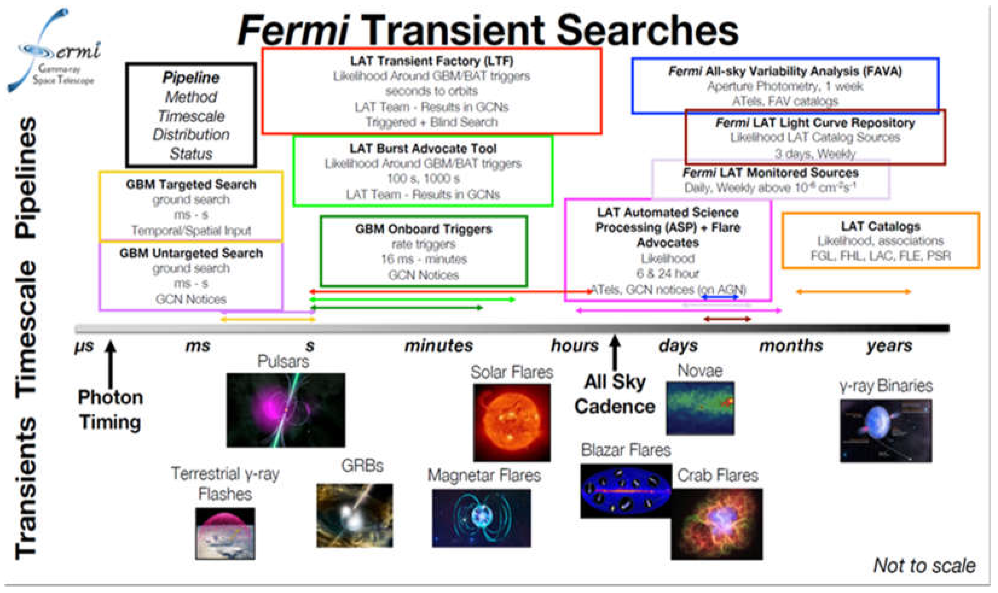
Figure 2.
SINBAD layout with the mirrors implemented to focus the IR photon beam: they are one ellipsoidal, two toroidal and three plane mirrors. Credit: DAΦNE-LIGHT Synchrotron Radiation Facility [103].
Figure 2.
SINBAD layout with the mirrors implemented to focus the IR photon beam: they are one ellipsoidal, two toroidal and three plane mirrors. Credit: DAΦNE-LIGHT Synchrotron Radiation Facility [103].
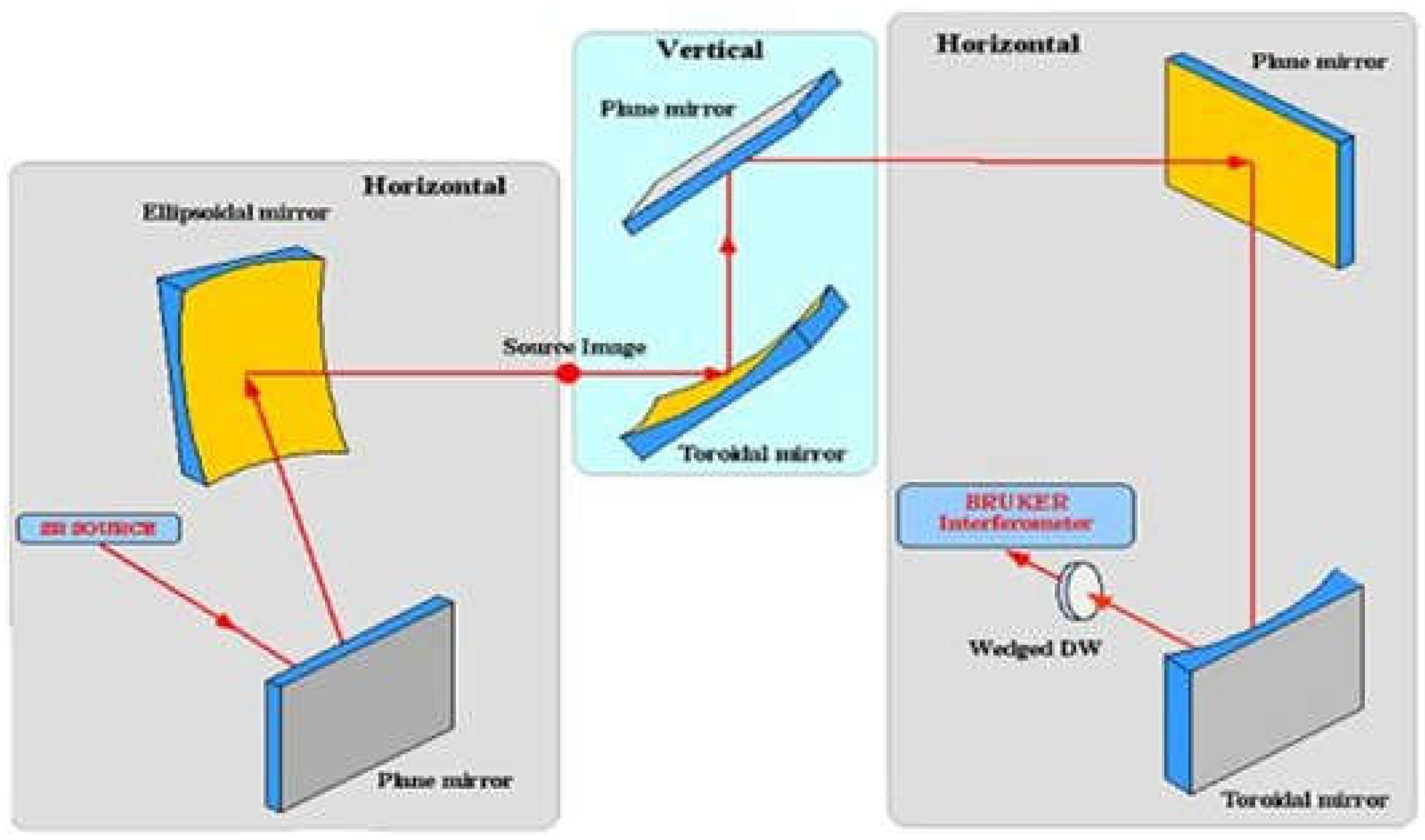
Figure 3.
Final optical layout with three additional external mirrors at SINBAD beamline. The infrared spot is visible on the mirror on the left.
Figure 3.
Final optical layout with three additional external mirrors at SINBAD beamline. The infrared spot is visible on the mirror on the left.
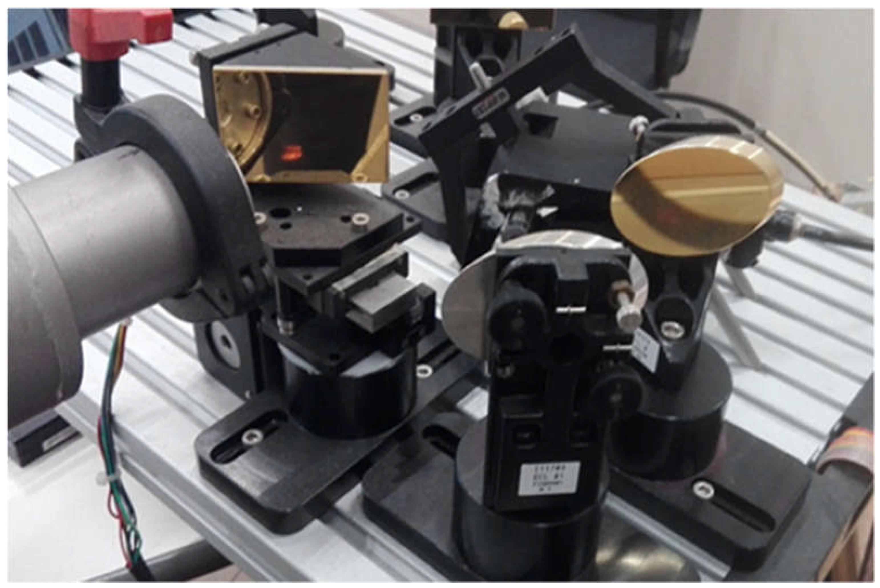
Figure 4.
DAFNE electron synchrotron light monitor (SLM) from the DAFNE control room. The SLM is a transverse device integrating the visible radiation emitted by the electrons by synchrotron acceleration. This type of detector does not show any evidence of bunches Credit: [79].
Figure 4.
DAFNE electron synchrotron light monitor (SLM) from the DAFNE control room. The SLM is a transverse device integrating the visible radiation emitted by the electrons by synchrotron acceleration. This type of detector does not show any evidence of bunches Credit: [79].
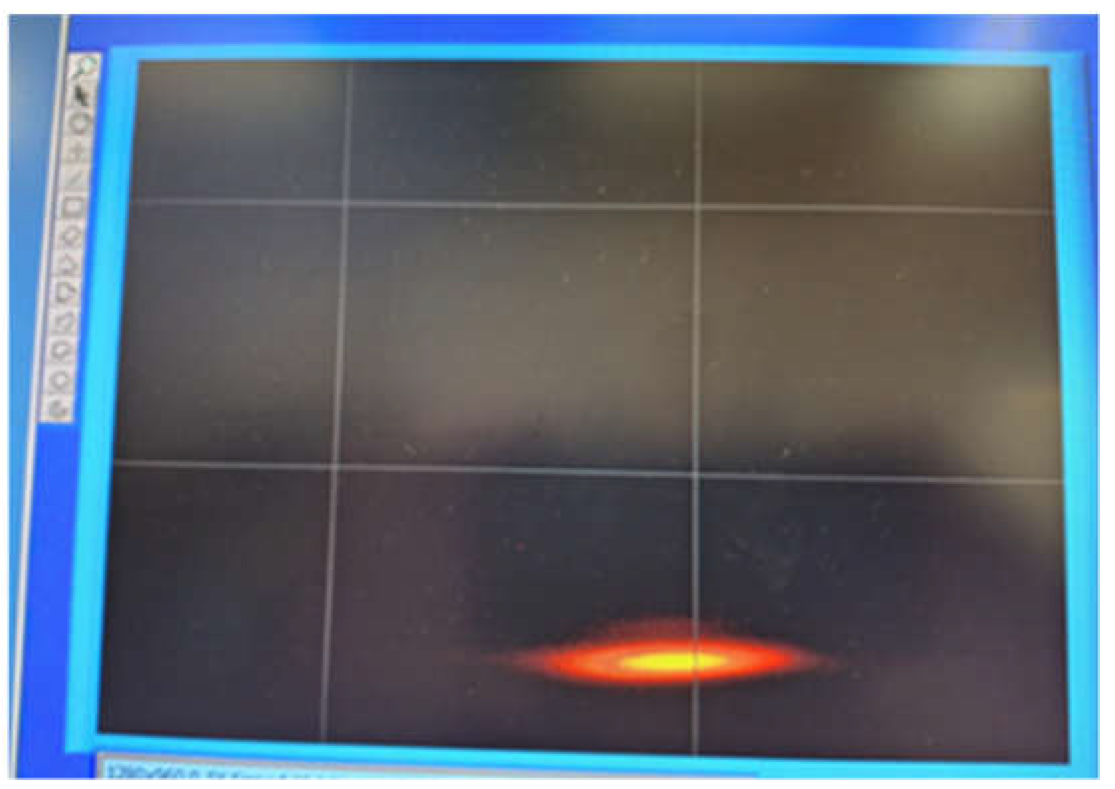
Figure 5.
Positron (red) and electron (blue) 110 bunches longitudinal amplitude detection versus time from two electromagnetic pickups connected directly to the oscilloscope and showing the separation of the bunches. Credit: [79].
Figure 5.
Positron (red) and electron (blue) 110 bunches longitudinal amplitude detection versus time from two electromagnetic pickups connected directly to the oscilloscope and showing the separation of the bunches. Credit: [79].
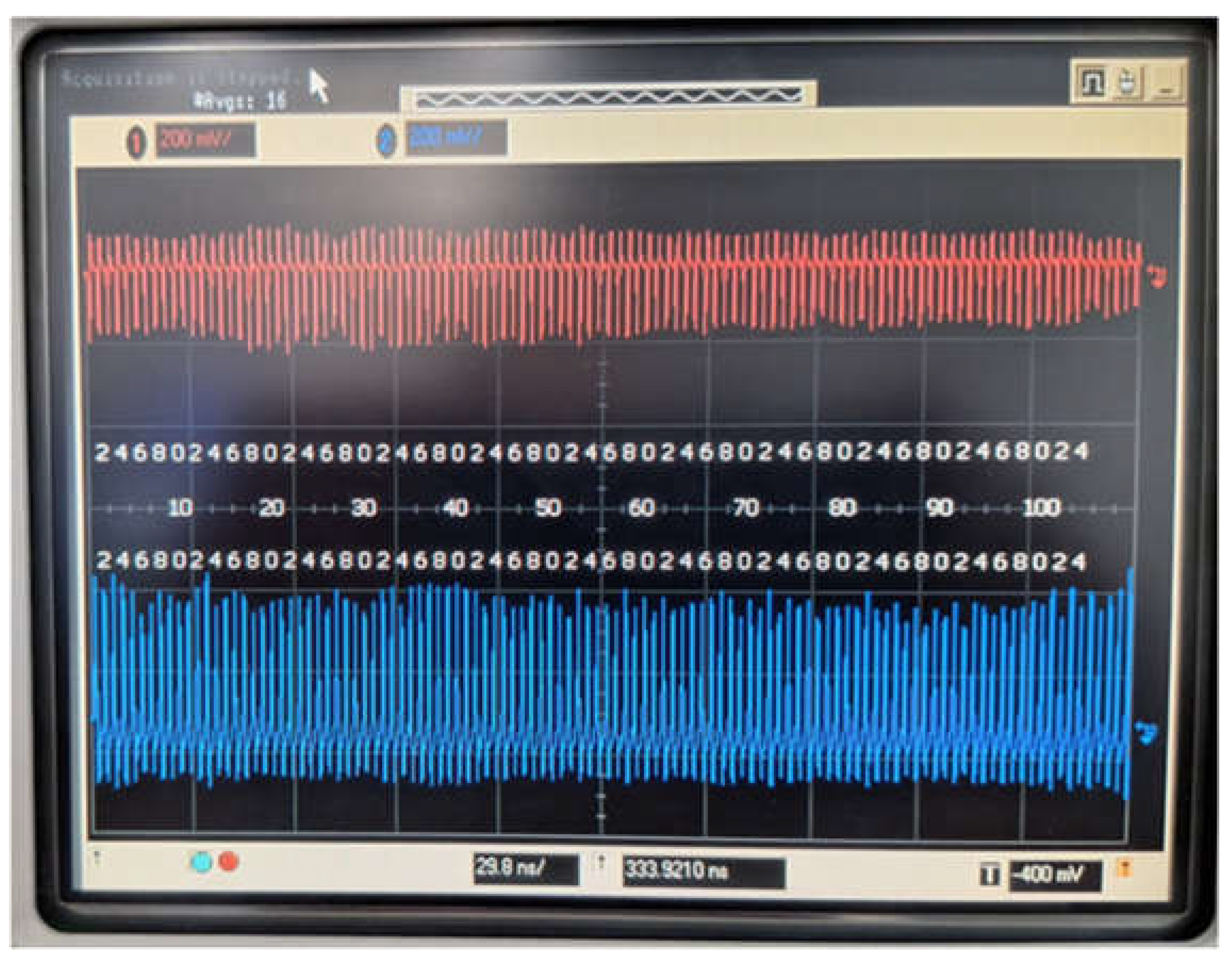
Figure 6.
Zoom of the e- bunches from the previous picture. The bunches are numbered. The plot shows the amplitudes in vertical versus the time in horizontal, the scale is 30 ns per square. Credit: [79].
Figure 6.
Zoom of the e- bunches from the previous picture. The bunches are numbered. The plot shows the amplitudes in vertical versus the time in horizontal, the scale is 30 ns per square. Credit: [79].
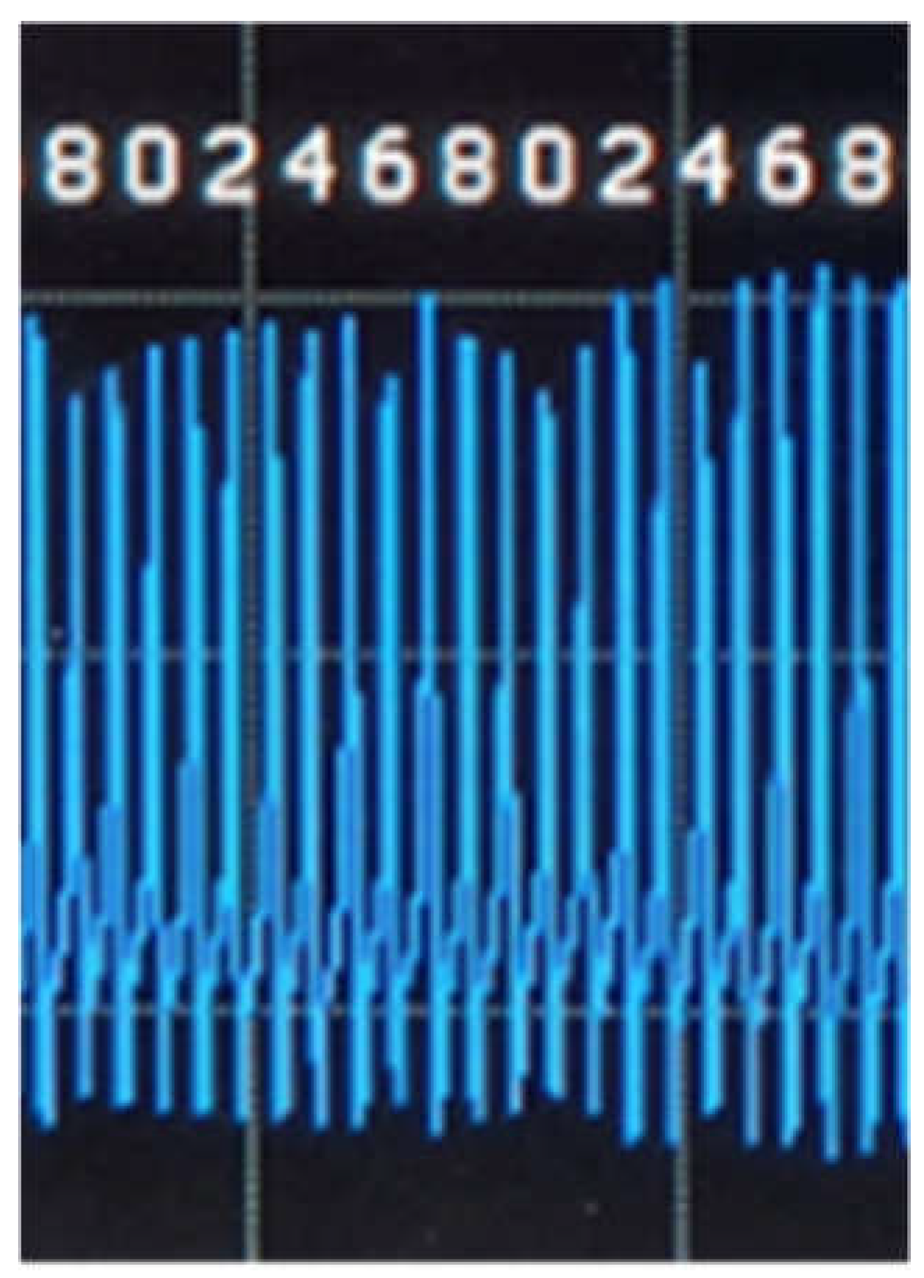
Figure 7.
Laboratory test to evaluate the effect of decreasing the temperature of MCT detector by applying a Peltier’s cell.
Figure 7.
Laboratory test to evaluate the effect of decreasing the temperature of MCT detector by applying a Peltier’s cell.
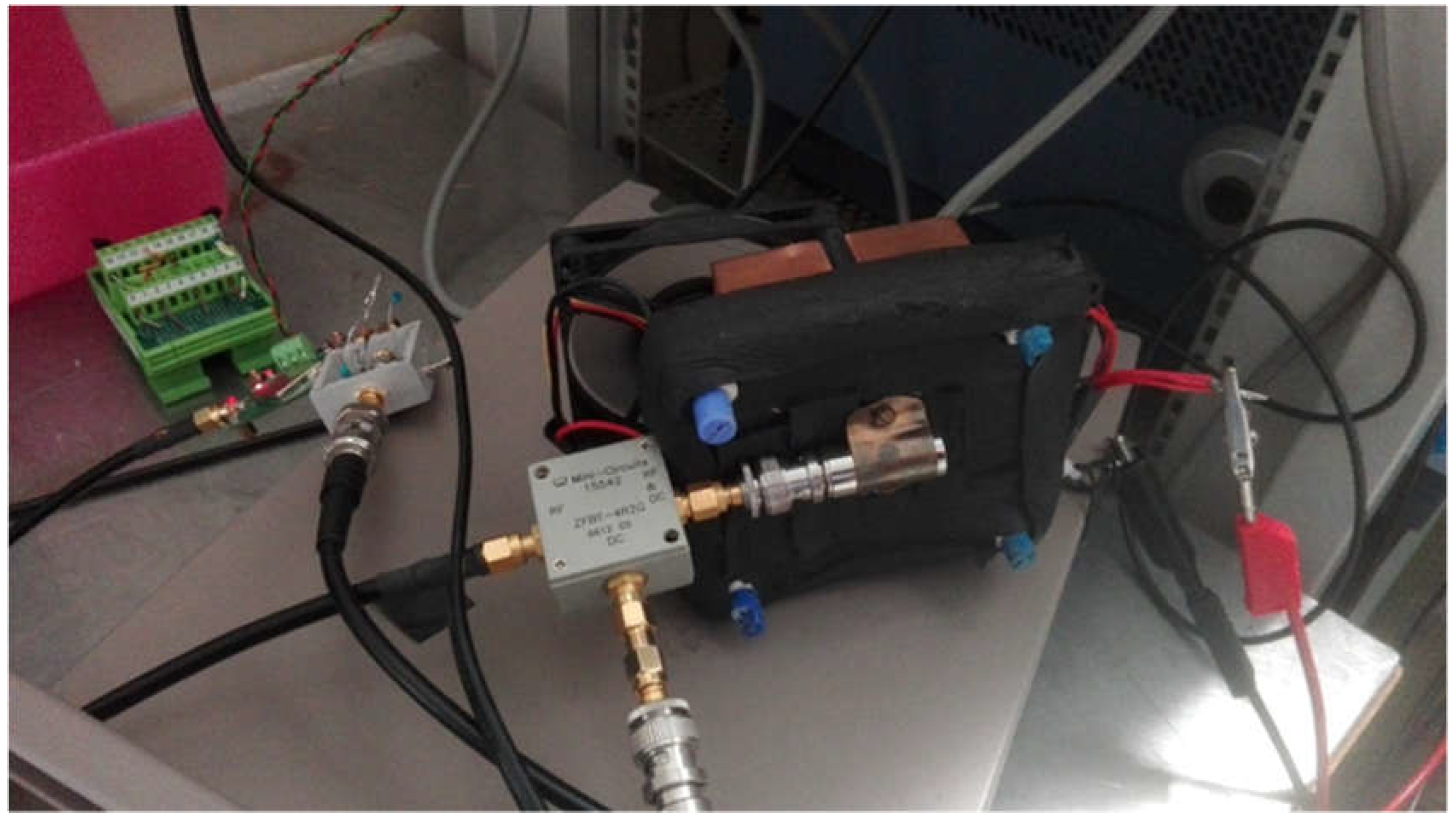
Figure 8.
Spectral response detectivity D* of PC10.6 photoconductor. VIGO catalog [149].
Figure 8.
Spectral response detectivity D* of PC10.6 photoconductor. VIGO catalog [149].
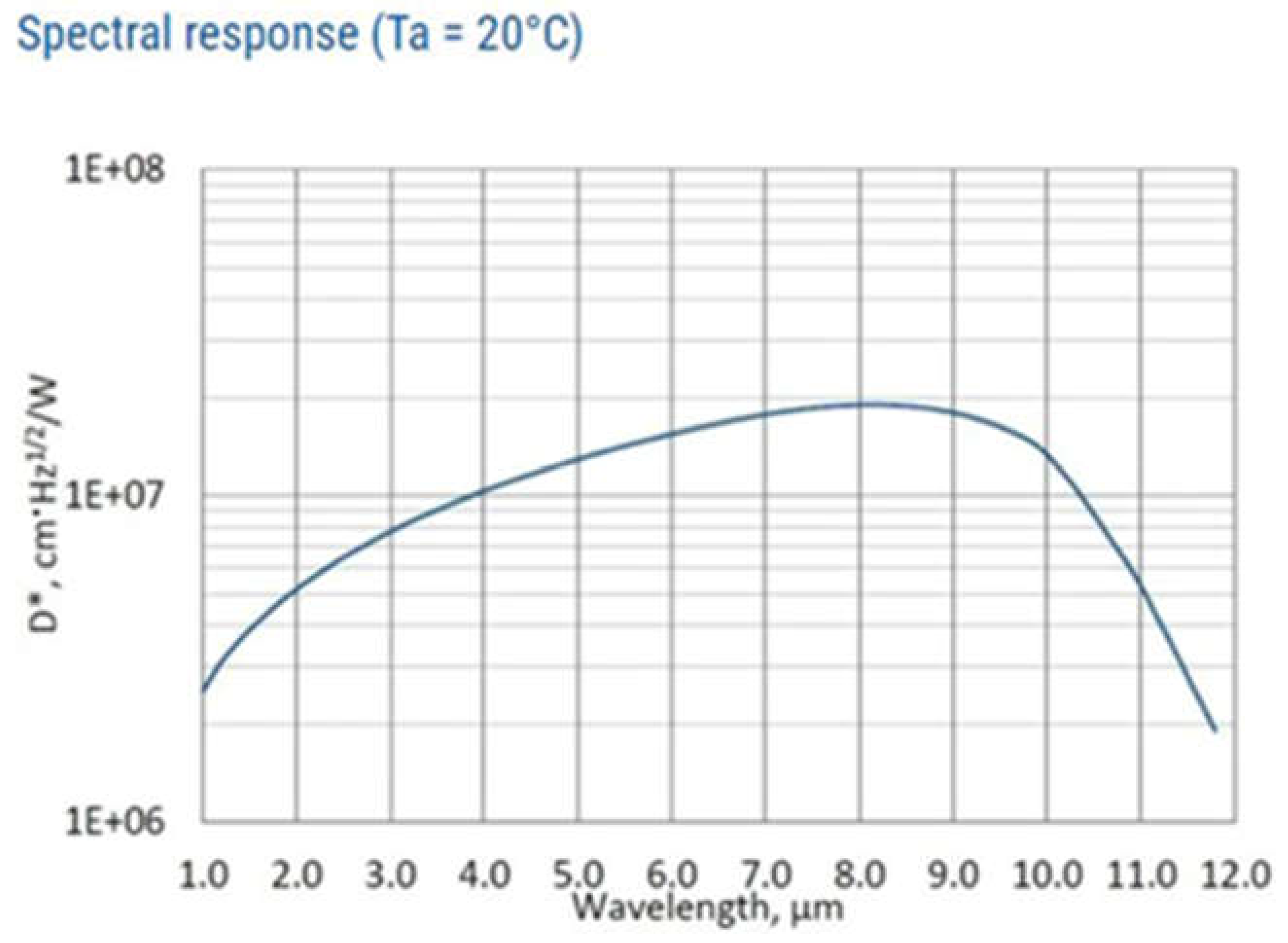
Figure 9.
VIGO PC10.6 photoconductor with BNC female package.
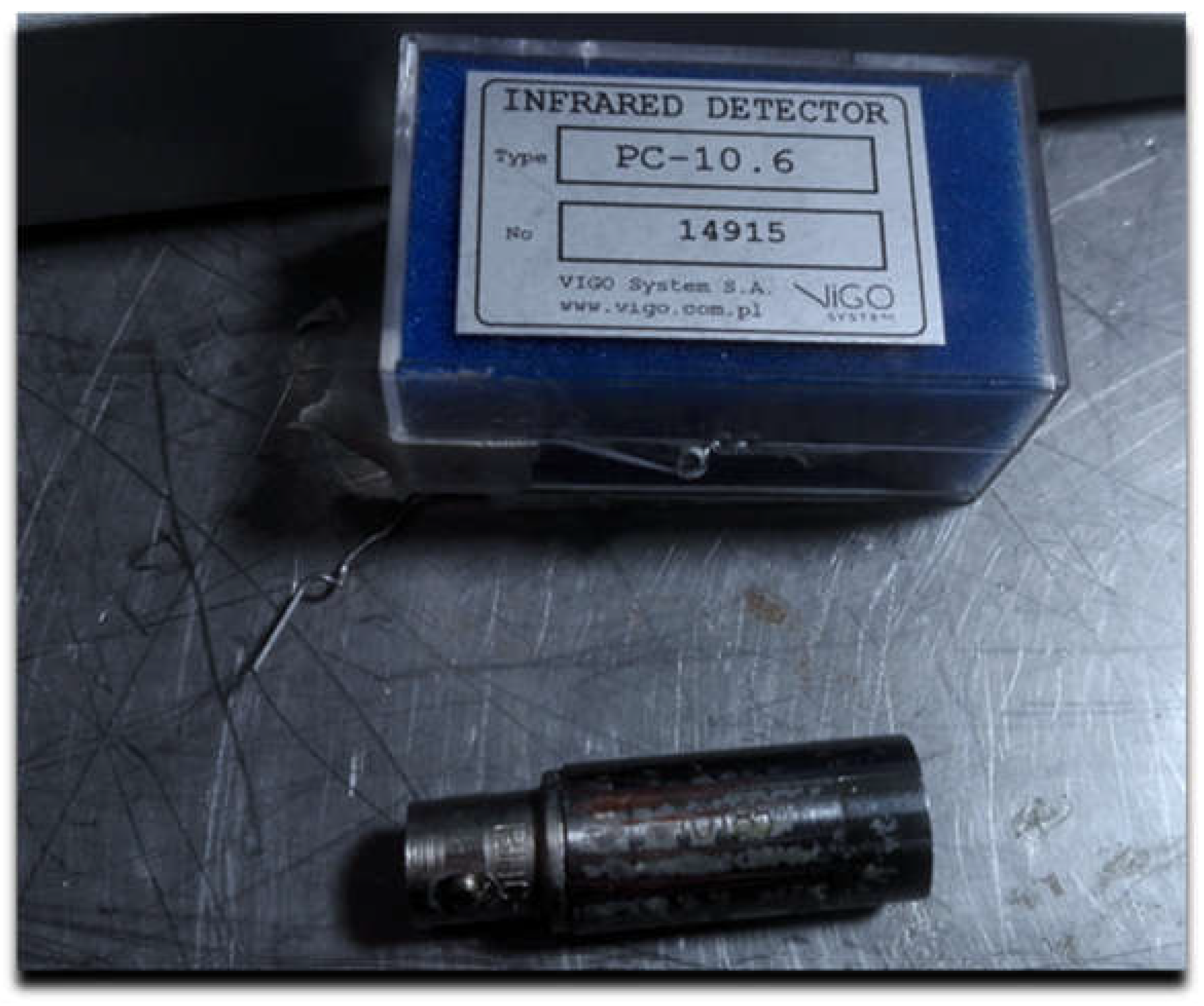
Figure 10.
Detectivity versus spectral response for InAsSb photovoltaic detectors P13894 by Hamamatsu data sheet [150].
Figure 10.
Detectivity versus spectral response for InAsSb photovoltaic detectors P13894 by Hamamatsu data sheet [150].
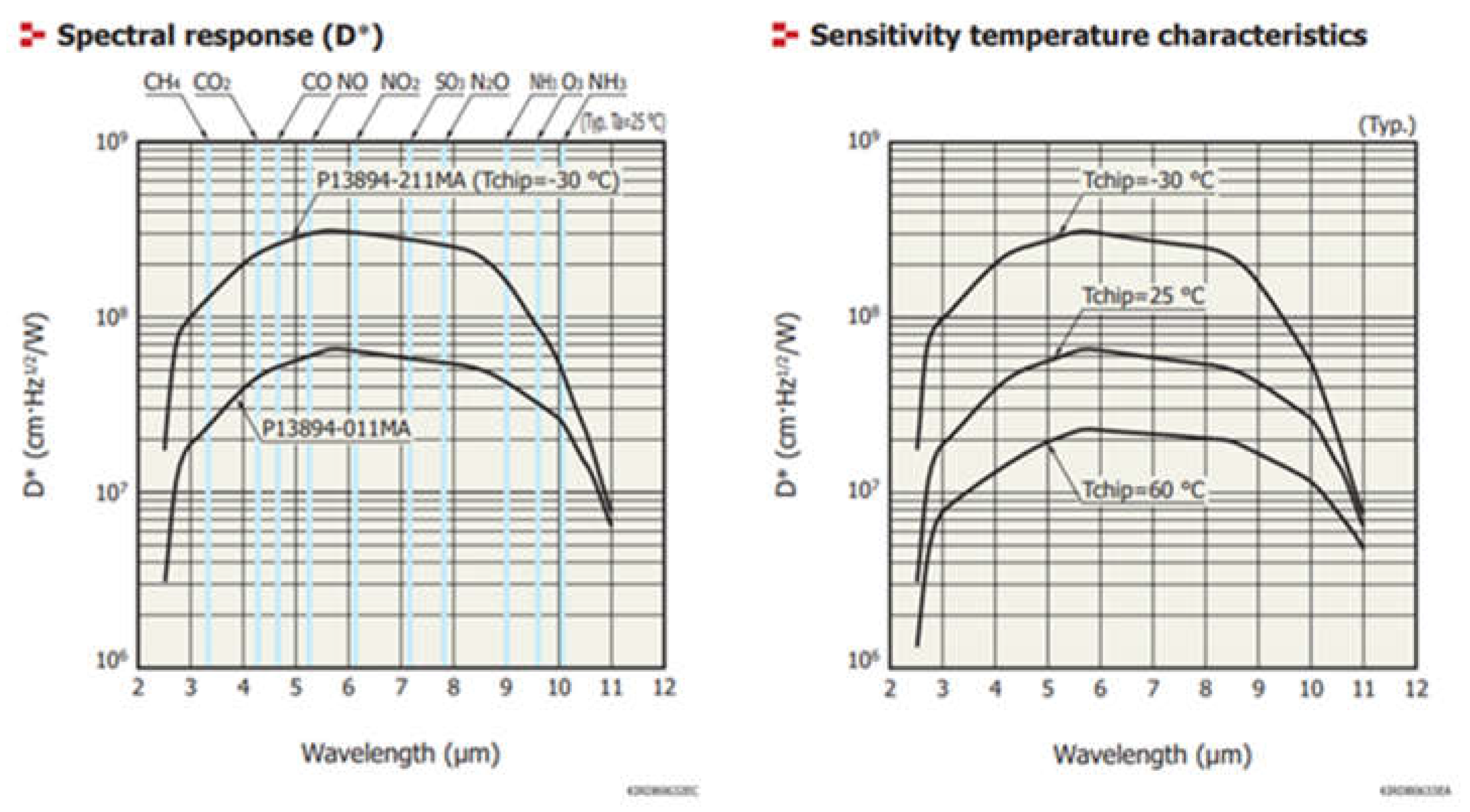
Figure 11.
Amplified MCT detector signal (cyan trace, 2mV per division), that reproduces the bunch train corresponding to the signal from the electromagnetic pickup (yellow trace of the oscilloscope). The red trace shows the machine master clock used as trigger.
Figure 11.
Amplified MCT detector signal (cyan trace, 2mV per division), that reproduces the bunch train corresponding to the signal from the electromagnetic pickup (yellow trace of the oscilloscope). The red trace shows the machine master clock used as trigger.
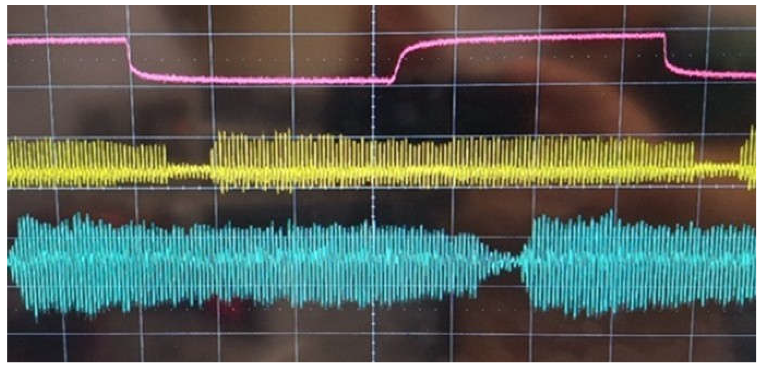
Figure 12.
The Hamamatsu detector between two Peltier cells.
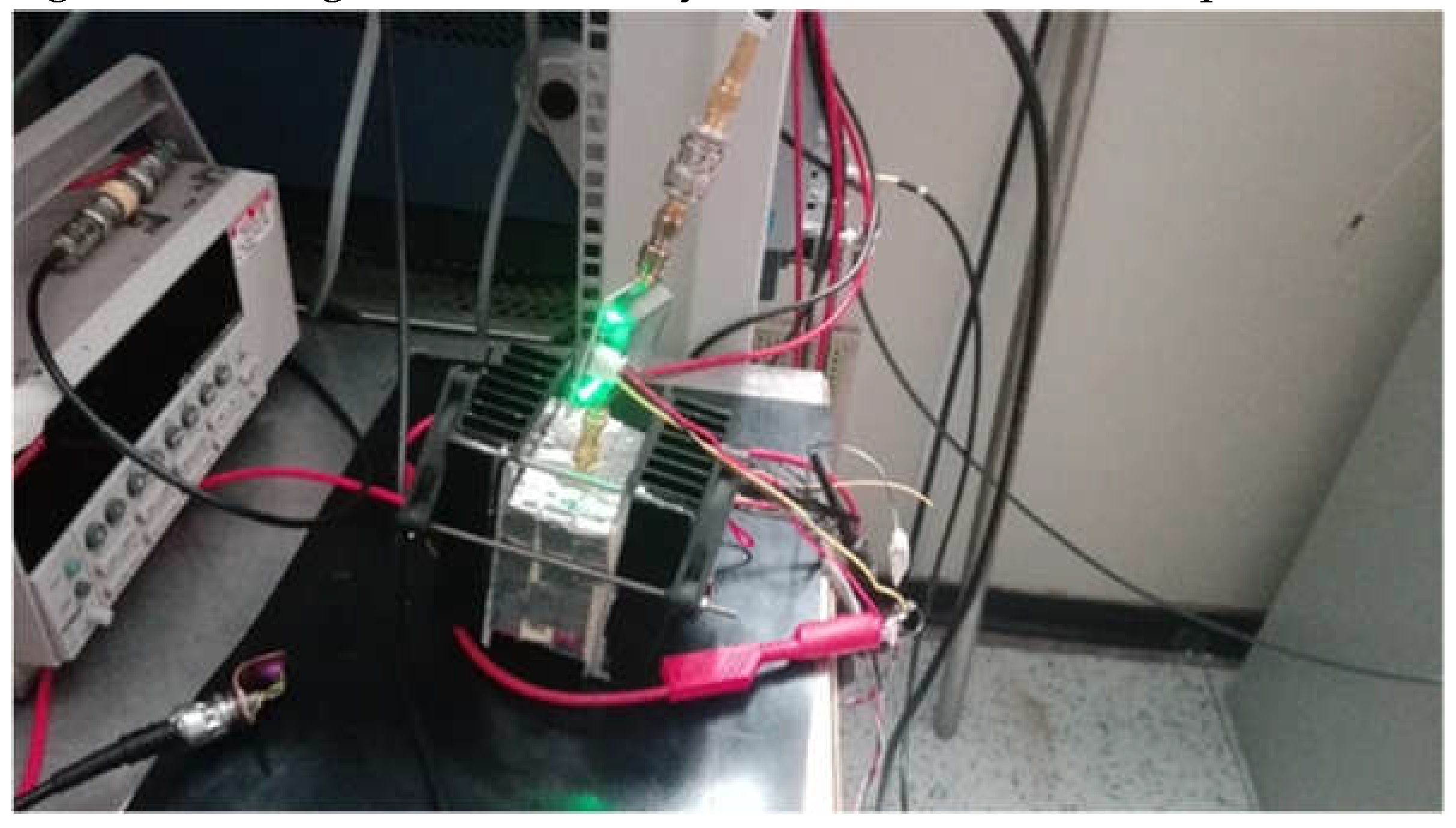
Figure 13.
The photovoltaic detector acquiring the synchrotron light (cyan trace, 2mV per division). In red the machine master clock, in yellow the beam signal coming from an electromagnetic pickup. Note that the difference of phase between the signals are not meaningful because the signals travel different paths.
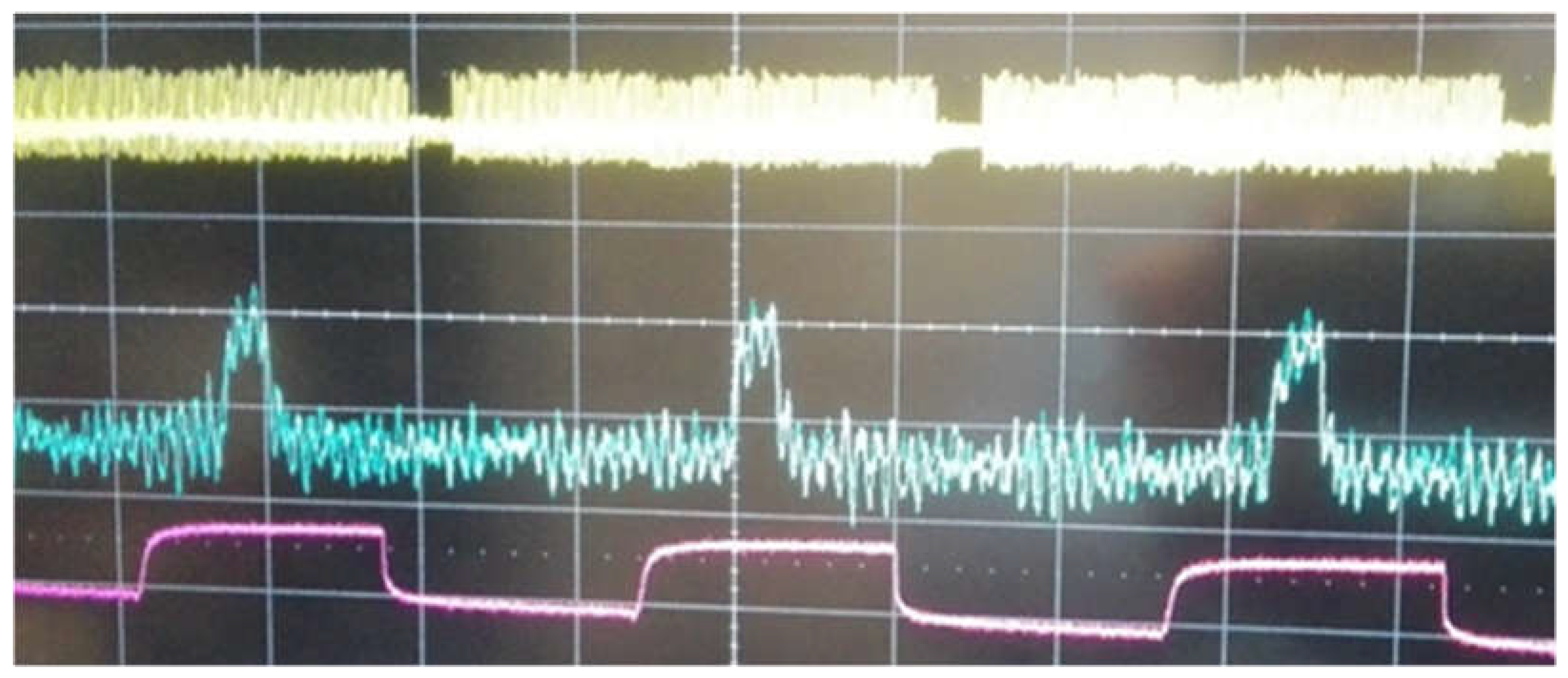
Figure 14.
From the analysis of data file 2024-7-31-17-44-48.txt: the classifier plotted time domain behavior (left/up), first derivative (right/up), second derivative (left/mid), absolute amplitude in frequency domain after Fast Fourier Transform (right/mid), real amplitude in frequency domain after FFT (left/down), imaginary amplitude in frequency domain after FFT (right/down).
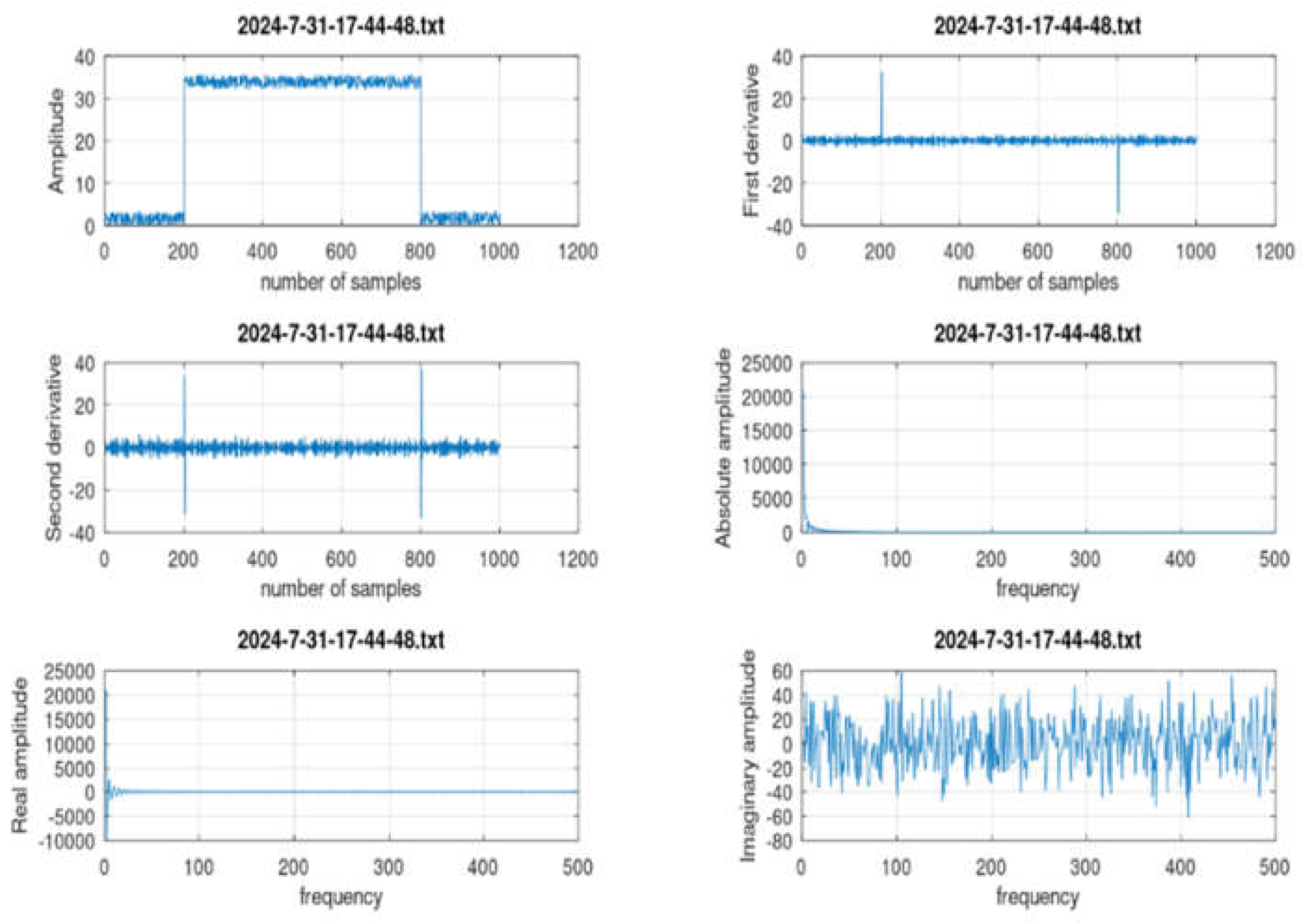
Figure 15.
From the analysis of data file 2024-7-31-13-13-20.txt: the classifier plotted time domain behavior (left/up), first derivative (right/up), second derivative (left/mid), absolute amplitude in frequency domain after Fast Fourier Transform (right/mid), real amplitude in frequency domain after FFT (left/down), imaginary amplitude in frequency domain after FFT (right/down).
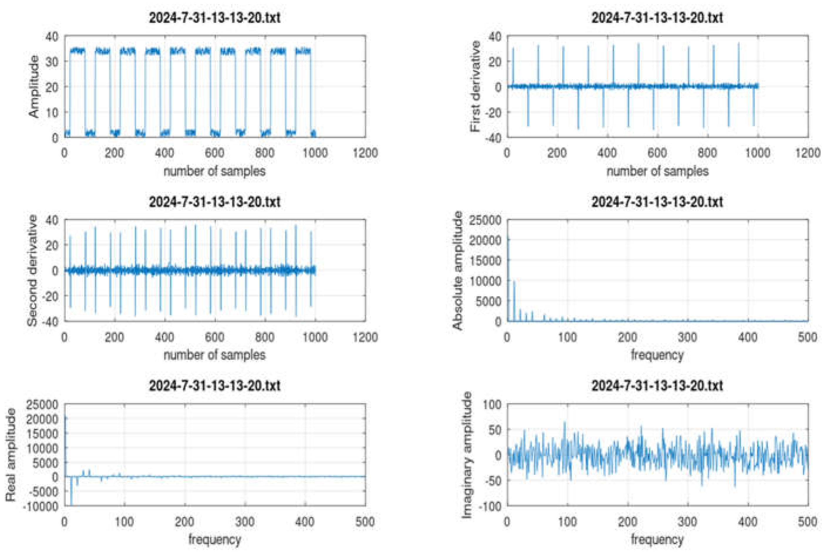
Figure 16.
From the analysis of data file 2024-7-31-13-15-46.txt: the classifier plotted time domain behavior (left/up), first derivative (right/up), second derivative (left/mid), absolute amplitude in frequency domain after Fast Fourier Transform (right/mid), real amplitude in frequency domain after FFT (left/down), imaginary amplitude in frequency domain after FFT (right/down).
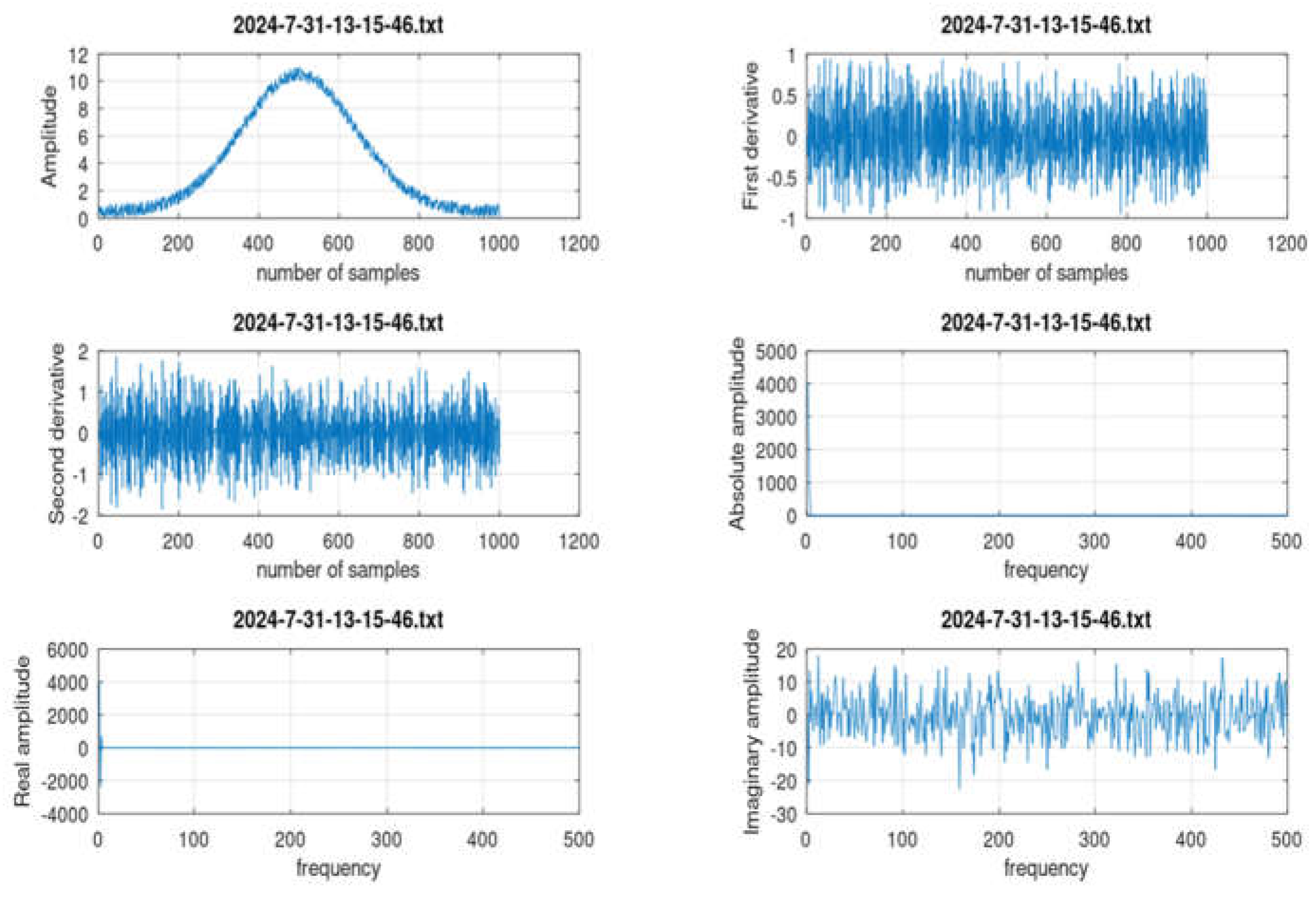
Figure 17.
From the analysis of data file 2024-7-31-18-24-20.txt: the classifier plotted time domain behavior (left/up), first derivative (right/up), second derivative (left/mid), absolute amplitude in frequency domain after Fast Fourier Transform (right/mid), real amplitude in frequency domain after FFT (left/down), imaginary amplitude in frequency domain after FFT (right/down).
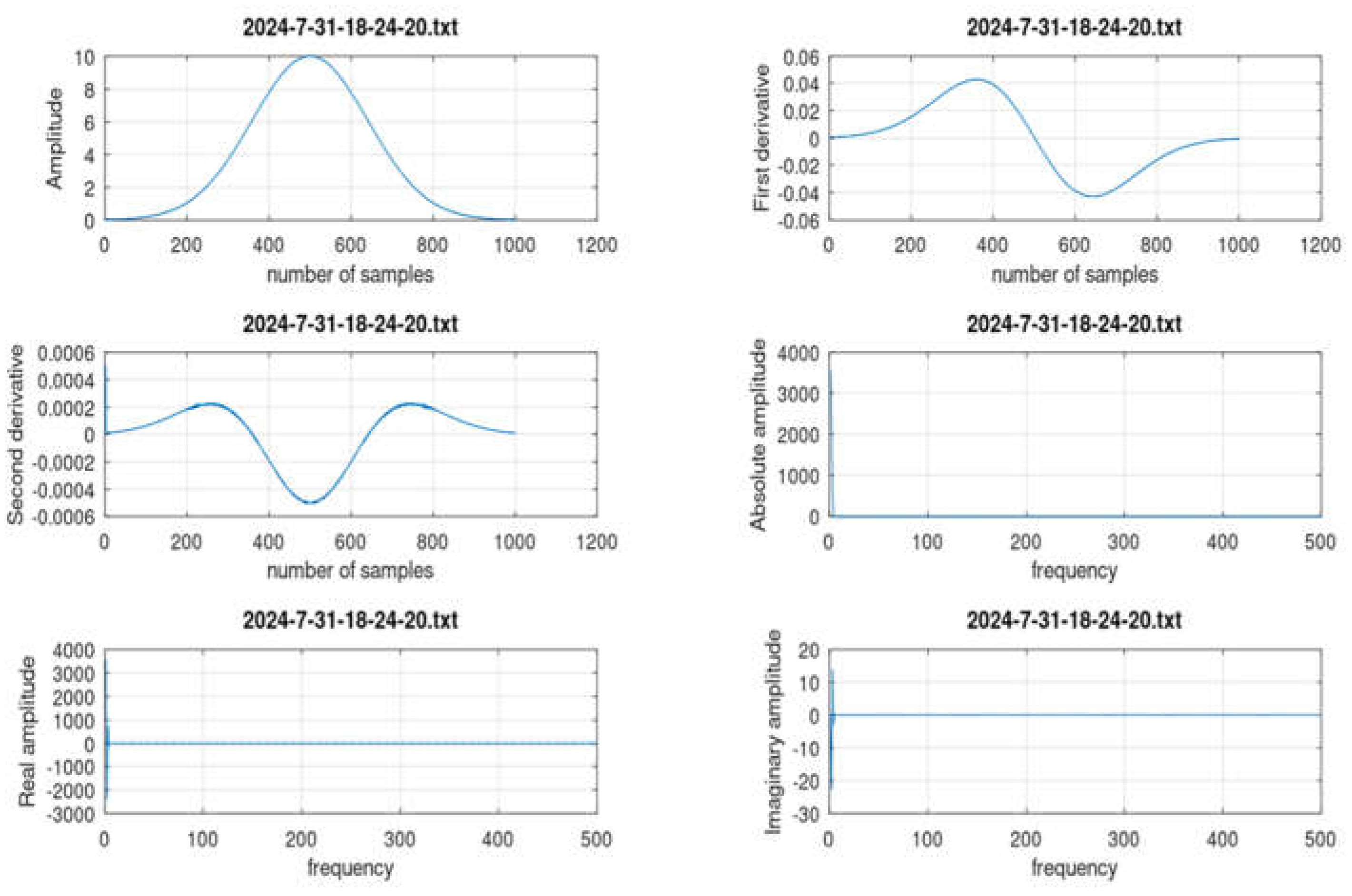
Figure 18.
From the analysis of data file 2024-7-31-18-0-36.txt: the classifier plotted time domain behavior (left/up), first derivative (right/up), second derivative (left/mid), absolute amplitude in frequency domain after Fast Fourier Transform (right/mid), real amplitude in frequency domain after FFT (left/down), imaginary amplitude in frequency domain after FFT (right/down).
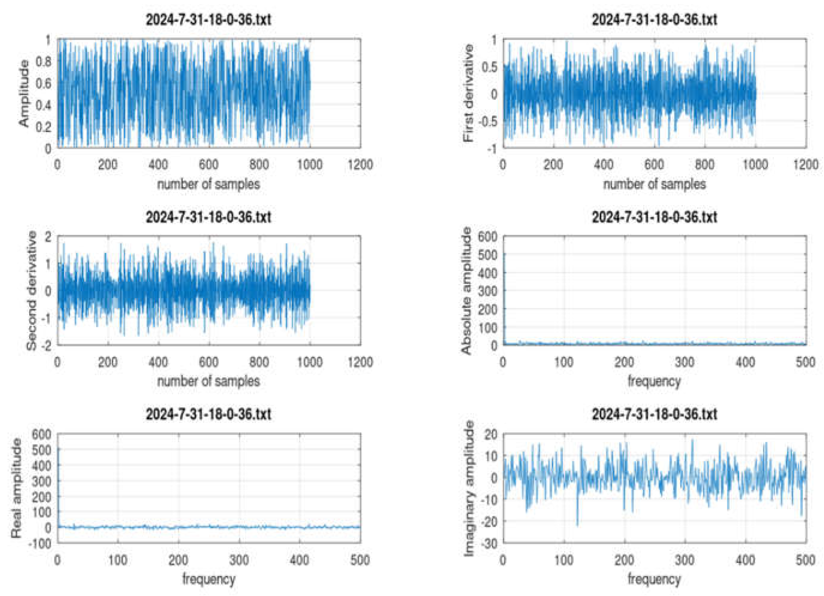
Figure 19.
From the analysis of data file 2024-7-31-18-12-9.txt: the classifier plotted time domain behavior (left/up), first derivative (right/up), second derivative (left/mid), absolute amplitude in frequency domain after Fast Fourier Transform (right/mid), real amplitude in frequency domain after FFT (left/down), imaginary amplitude in frequency domain after FFT (right/down).
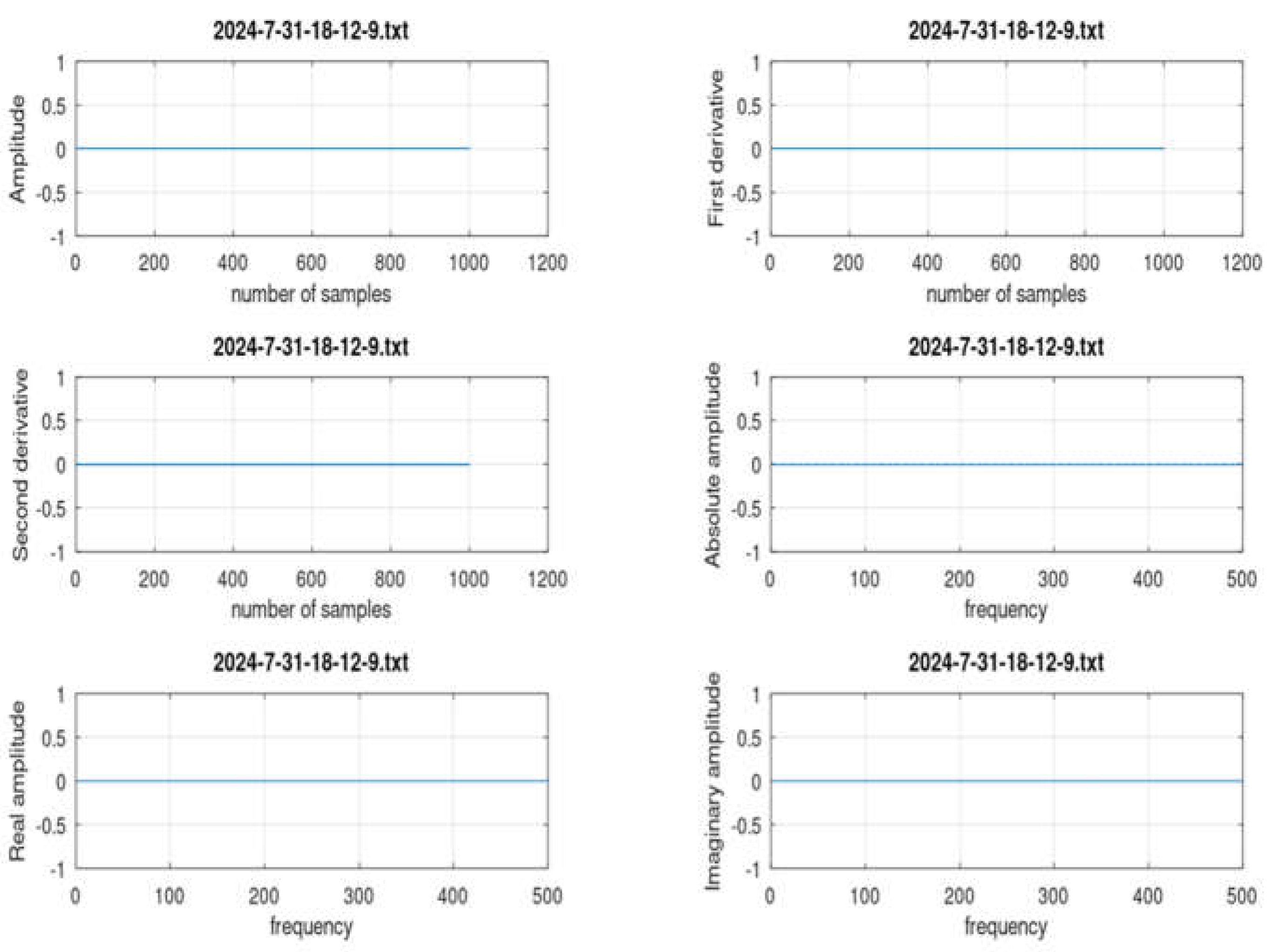
Figure 20.
From the analysis of data file 2024-7-31-18-15-49.txt: the classifier plotted time domain behavior (left/up), first derivative (right/up), second derivative (left/mid), absolute amplitude in frequency domain after Fast Fourier Transform (right/mid), real amplitude in frequency domain after FFT (left/down), imaginary amplitude in frequency domain after FFT (right/down).
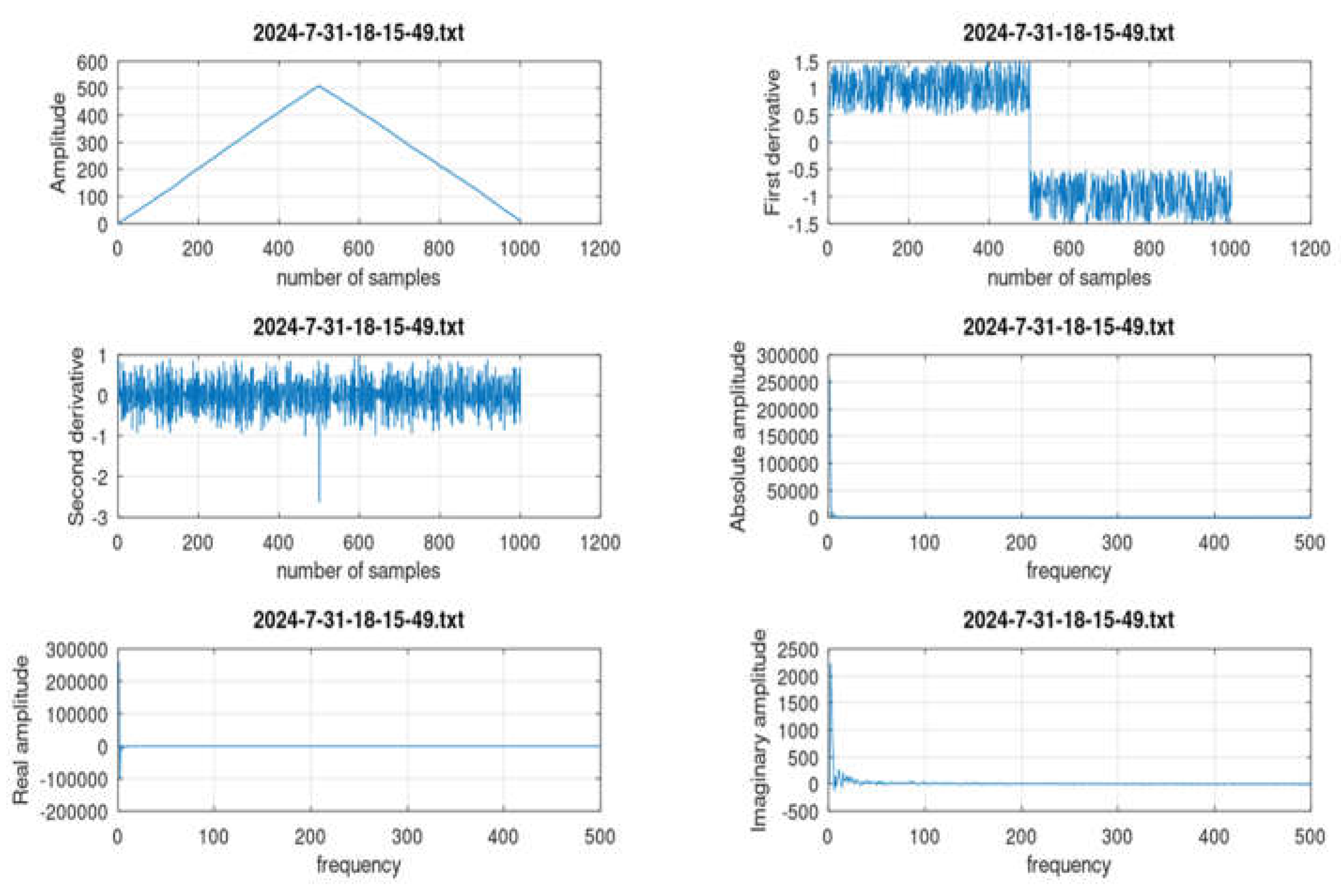
Figure 21.
Flow chart summarizing the modules discussed. The implementation of noise cancelling filters is included inside the two red blocks (firb_classifier and ANN).
Figure 21.
Flow chart summarizing the modules discussed. The implementation of noise cancelling filters is included inside the two red blocks (firb_classifier and ANN).
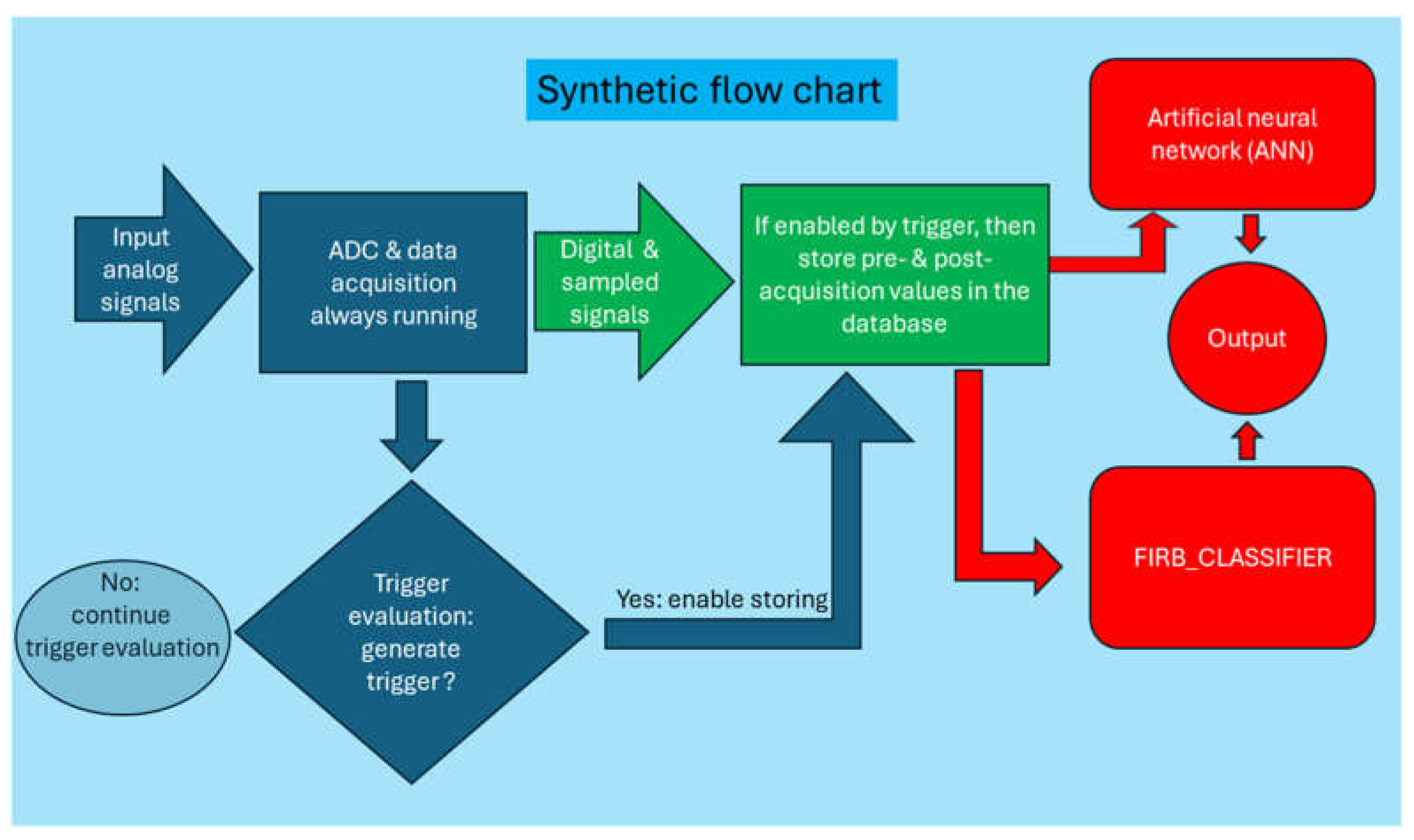
Disclaimer/Publisher’s Note: The statements, opinions and data contained in all publications are solely those of the individual author(s) and contributor(s) and not of MDPI and/or the editor(s). MDPI and/or the editor(s) disclaim responsibility for any injury to people or property resulting from any ideas, methods, instructions or products referred to in the content. |
© 2025 by the authors. Licensee MDPI, Basel, Switzerland. This article is an open access article distributed under the terms and conditions of the Creative Commons Attribution (CC BY) license (http://creativecommons.org/licenses/by/4.0/).
Copyright: This open access article is published under a Creative Commons CC BY 4.0 license, which permit the free download, distribution, and reuse, provided that the author and preprint are cited in any reuse.


