
Submitted:
23 January 2025
Posted:
24 January 2025
You are already at the latest version
Abstract
Hazardous materials events by rail have the characteristics of small probability and even higher consequence than other modes. In response to these characteristics, we have adopted conditional value-at-risk into the risk assessment of hazardous materials railway transportation, which can flexibly realize the configuration decisions from risk neutrality to risk aversion. Moreover, this paper not only focus on risk reduction, but also pay more attention to reasonable risk distribution, which means risk equity for people in the entire environment. In this paper, a new model is proposed by adding risk equity goal to the traditional conditional value-at-risk assessment, and route decision-making can be optimized through this model, then an algorithm based on k-shortest path algorithm is given to solve the problem. Finally, the validity of the model and algorithm is verified based on the example of hazardous materials railway transportation network in the Yangtze River Delta. This research can provide decision support for enterprises to optimize the route of railway transportation of hazardous materials, and can also provide decision support for the government to carry out detailed safety management of railway transportation of hazardous materials.
Keywords:
hazardous materials
; railway transportation
; risk equity
; CVaR
; route optimization
1. Introduction
Hazardous materials transportation, despite the possible hazards, is a necessary part of industrial production activities. As one of the important methods of transportation, railway has been exploited to transport hazardous materials (Hazmat) to ensure the industrial supply chain circulation. Over the past two decades, objective conditions and institutional system of hazardous materials railway transportation become gradually mature. According to statistics, around 114,005 train accidents were reported from 2011 to 2020, where 70,432 cars carrying Hazmat were involved; of these 6,854 cars were damaged or derailed and 425 released Hazmat, which translates into an average 42.5 cars involved in Hazmat release incidents every year in United States [1]. As of 2022, China's annual shipment of hazardous chemicals is estimated to amount to 1.8 billion tons, with approximately 180 million tons transported by rail [2]. On May 23, 2017, a hazardous chemicals transportation explosion occurred in a tunnel on the Zhangshi Expressway in Baoding, Hebei, resulting in 15 deaths and damage to vehicles [3]. In another incident, on February 3, 2023, a freight train carrying hazardous materials derailed in East Palestine, Ohio, USA, causing the death of nearly 44,000 animals, according to data from the Ohio Department of Natural Resources [4]. Though Bubbico et al. [5] have proved it safer transport Hazmat by rail, Hazmat events still have the characteristic of low probability-high consequence, which makes effective risk assessment always a problem. Expected consequence (Traditional Risk model) is risk-neutral, so it is impossible to develop a risk aversion route that would prevent high consequence events.
There have been abundant literature on risk assessment of Hazmat transportation. Abkowitz et al. [6] established a Perceived Risk (PR) model by introducing the risk preference parameter q into Traditional Risk (TR) model to reflect the degree of risk preference of decision makers. As we have found that people’s risk aversion to disasters such as hazardous material accidents is objective, and their aversion to the consequences of larger accidents is deeper than that of events with high probability and small consequences, the model is very close to realistic decision making. However, it is difficult to determine appropriate risk preference parameter q in actual production and scientific research activities. Erkut and Ingolfsson [7] introduced three different catastrophe avoidance models, namely minimizing the maximum risk, minimizing the variance of results between routes, and an explicit disutility function. Verma and Verter [8] used Gaussian Plume Model to estimate the people exposure risk of the worst-case in the risk assessment of Hazmat railway transportation. With the help of or partially improving these risk assessment models, scholars have done research on route selection and location decision-making for hazardous materials road transportation and even multimodal transportation under various scenarios [9,10,11,12,13].
Kang et al. [14] proposed Value-at-risk (VaR) model to assess the risk of dangerous goods transportation. Fang et al. [15] further demonstrated the application of VaR in multi-hazmat railcar routing, highlighting its effectiveness in optimizing route risks. Meanwhile, Conditional Value-at-Risk (CVaR), as an extension of VaR, quantifies extreme losses exceeding the mean value of VaR [16]. Since then, scholars have studied the use of CVaR for dynamic route and scheduling decisions in Hazmat transportation networks [16,17]. The CVaR is originally applied for financial portfolio optimization in the financial field [18]. Based on the widespread application of CVaR in risk-averse decision-making, Huang et al. [19] constructed a supply chain transportation network to analyze suppliers' risk aversion under stochastic pricing and information asymmetry. They proposed an emergency quantity discount contract to coordinate the supply chain. To address uncertainties in dynamic environments, Ma et al. [20] integrated CVaR into a blockchain-enabled supply chain finance system, investigating revenue optimization under centralized and decentralized decision-making models. This further demonstrated the applicability of CVaR models in complex decision-making scenarios. Hosseini and Verma [21] proposed a CVaR-based risk assessment methodology for rail Hazmat shipments and even provided a clear definition of CVaR for Hazmat shipments. Zhong et al. [22] proposed a new model that includes conditional value at risk with regret (CVaR-R) as a risk measure that considers both the reliability and unreliability aspects of demand variability in the disaster relief facility location and vehicle routing problem. Su [23] incorporated CVaR risk measurement to Hazmat network design and achieved good research results.
In recent years, with the occurrence of Hazmat accidents, the problem of risk unfairness has aroused widespread concern among the public and society. Scholars use two ways of modeling to solve the problem of risk equity: one is to directly limit the risks related to the relevant population area by setting thresholds as constraints [24,25], and the other way to implement risk equity is setting risk equity goal [26]. Besides these, Fontaine et al. [27] proposed a new population-based risk definition and an objective function for achieving risk equilibrium. Hosseini and Verma [28] proposed an analytical framework that makes use of a conditional value-at-risk (CVaR) measure of risk to generate shortest risk shipment routes while promoting risk equity in both the arcs and the yards of the railway network. However, the approach that they used setting risk equity constraints for each yard and each arc is no longer popular. Because it is difficult to determine a reasonable risk threshold in large-scale instances, this method has been gradually replaced by setting risk equity goal in recent literature.
Using CVaR minimized as the goal is to pay attention to serious consequences to achieve risk aversion. This will make the system decision avoid extreme high consequences. However, this goal can only ensure that the accident consequence of a single road section or node is minimized, and it cannot achieve a balanced distribution of risks between road sections and nodes. Setting risk equity goal should enable groups that are susceptible to risk unfairness (those groups are generally located geographically on risky routes or near stations) to reduce risk as much as possible. Combining it with the goal of minimizing CVaR means that the overall risk is minimized, but also partial risk reduction must be achieved. It can better achieve risk avoidance. Therefore, we propose conditional value-at-risk with equity (CVaRE) as a combination of CVaR and risk equity goal, while reducing the frequency of extreme high consequences and higher risk.
This article has made the following contributions to solve the above problems:
- We introduce CVaR into risk assessment in railway transportation scenarios for risk aversion routes and dispatch decisions.
- Taking into account the risk unfairness of the external public, we have added risk eq-uity goal to the CVaR-based assessment, and proposed a new model named condi-tional value-at-risk with equity (CVaRE).
- We introduce a practical example, and use the k-shortest CVaRE algorithm to solve the problem model, generating the optimal solution. This can serve as a guide and reference for railway hazardous materials transportation dispatch decision-makers.
The remainder of this paper is organized as follows. In Section 2, we define the research questions and basic assumptions, give the notations of sets, parameters and variables, and provide the basic definition of CVaR and the scenarios in this article. Section 3 respectively provides a direct transportation model, a transfer transportation model, and finally an outline of solution methodology based on k-shortest path algorithm. Section 4 uses the railway infrastructure of railway operators to generate actual-scale calculation examples, which are solved and analyzed to obtain management insights. Conclusion and directions of future research are outlined in Section 5.
2. Problem Description
2.1. Assumptions and Notations
2.1.1. Assumptions of Railway Transportation System
In the railway transportation system, the physical infrastructure includes railway yards and tracks. Any two railway stations are connected by tracks, and a series of service sections and intermediate stations constitute the itinerary that the railcar can use for its itinerary. In the transportation of hazardous materials, there are two cases: direct transportation and transfer transportation. Direct transportation will not stop at any station, and transfer transportation (as Figure 1 depicts) will only stop at fixed yard(s) (could be called marshalling yard(s)) and be remarshalled.
The problem we need to solve is the train transportation route and re-marshalling plan of the railway company, which regularly transports Hazmat between different origins and destinations, and needs to ensure that the needs are met. Therefore, the goal is to use conditional value-at-risk method and conditional value-at-risk with equity method to determine Hazmat railway transportation routes and possible regrouping stations and plans so that hazardous materials risks are minimized and distributed fairly in the railway network.
2.1.2. Notations
The railway transportation network is represented by a graph , where is the set of yards. is the set of arcs in the network, representing the connections between yards or between a yard and a marshalling yard. is the set of railway shipments, which flow between railway yards or between yards and marshalling yards. This network structure supports the transportation of hazardous materials by modeling both direct shipments and transfer shipments through intermediate marshalling yards. The specific definitions of the symbols are provided below:
Sets and indices
| Set of yards, indexed by i, j, k | |
| Set of marshalling yards, indexed by k, | |
| Set of arcs in the network, indexed by (i, j), (k, j) | |
| Set of railway shipments between railway yards(or yard and marshalling yards), indexed by v | |
| Set of yards in service of shipment v | |
| Set of arcs in service of shipment v |
Parameters and Variables
| Cost of moving a Hazmat container on arc (i, j) in shipment v | |
| Exposure risk of moving a Hazmat container on arc (i, j) in shipment v | |
| Exposure risk of using yard k for a Hazmat container in shipment v | |
| Origin of shipment v | |
| Destination of shipment v | |
| Non-negative integer, number of Hazmat containers in shipment v | |
| Confidence level, but also represents the level of risk aversion of suppliers | |
| Risk consequences in shipment v on arc (i, j) in shipment v | |
| Accident probability on arc (i, j) in shipment v | |
| Risk consequences of using yard k for Hazmat shipment v | |
| Probability of accident in using yard k | |
| Select Route VaR Threshold Under CVaR* | |
| 0-1 variable, whether to select arc (i, j) in shipment v as transportation section | |
| 0-1 variable, whether to select yard k as railway yard in shipment v | |
| Number of containers in shipment v unload at Marshalling yard k | |
| Delivery time associated with shipment v | |
| Time for handling containers at marshalling yard k | |
| Time for running on the railway route | |
| Impact radius of Hazmat accident | |
| Maximum population density of the area passed through by arc (i, j) | |
| Population density of the area where yard k is located |
2.2. Hazmat Risk Measurement Formulation Based on VaR and CVaR
CVaR is based on VaR. VaR refers to the maximum possible loss value of a certain financial asset or portfolio within a certain holding period under a certain confidence level. It focuses on a certain point of confidence, while ignoring the underlying risk beyond that point. Compared with VaR, CVaR satisfies the consistency axiom, and pays attention to the risk of exceeding the base point. Therefore, soon after scholars introduced VaR in the Hazmat transportation, they introduced CVaR into the risk assessment of Hazmat transportation.
Given that be the discrete random variable denoting the risk associated with O-D pair O(v)-D(v), be the smallest value in the set {}, be the corresponding probability.
where .
Given the confidence level , VaR is the minimal threshold level such that the hazmat risk does not exceed with the least probability of :
Note that , where always
Then
can be simplified as , which is minimal loss value for decision-making shipment v under the confidence level . When , we define equal to 0; then . Therefore, the VaR risk of O-D pair O(v)-D(v) has .
There is a shipment v for a specific O-D pair, can be written as . Therefore, a discrete CVaR assessment (4) for each O-D pair is established for the transportation of hazardous materials.The consequences of the risk are measured by road segments; the corresponding consequence for each road segment (i, j), is ; the corresponding probability is ; then
Note that .
The optimal conditional risk value for a specific O-D pair can be expressed as follows [29]:
For N is set of midpoints in the network, indicates whether to choose a route for transportation;
Because of the optimal content , that is, the optimal VaR is between the risk of the minimal road segment and the risk of the maximum road segment, and the risk values ,of all the road segments of are sorted in ascending order and defined separately as ,where is the minimal value of ,. The values of must be fixed, and the objective function becomes a linear function. Therefore,
After determining the values’ range of, it can be converted into a linear function. Since the CVaR function is convex, that is, it is consistent with . Generally speaking, in the calculation of CVaR. From (7) we can see that different corresponding to different CVaR values, the optimal CVaR corresponds to the optimal VaR.
3. Model Establishment
3.1. Mathematical Model
In this section, we outline the model of Hazmat railway transportation system in direct transportation case and transfer transportation case.
3.1.1. Model Based on CVaR of Direct Transportation Case (Base Case)
We call the Hazmat railway transportation problem of direct transportation case (base case) problem (P). The proposed problem (P) is formulated below.
(P)
Subject to
The model is a bi-objective model: the objective function (8) is minimizing total CVaR for all the shipments; (9) is to minimize the total cost of Hazmat transportation, which includes cost of moving Hazmat on arc (i, j). Constraint (10) represents CVaR in shipment v, among them, ; Constraint (11) is flow balance equation for any (i, j) ϵ A. Equation (12a)(12b) represent respectively the accident consequences of exposure risk on arc (i, j) and yard k.
The model P is aimed at the simple direct transportation problem (there is no stopover in this type of problem). In fact, the railway has a marshalling station for the reorganization, transfer and delivery of trains on the railway. In the strict management system of railways, the arrival and departure of hazardous materials carriages can only be carried out on special railway lines and marshalling yards, so Hazmat railway transportation excludes halfway stations of the non-marshalling station.
3.1.2. Model Based on CVaRE of Transfer Transportation Case Considering Risk Equity
With the awakening of risk awareness among the government and the masses, it is necessary to consider risk equity in the railway transport of Hazmat. CVaR emphasizes the risk caused by the part of the accident result greater than , and minimizing CVaR can effectively reduce the risk of super-large results and achieve a certain risk equity. However, the consideration of risk equity in this part, especially the determination of and α , relies on the subjective evaluation of decision makers, and minimizing CVaR is the perceived risk equity to a certain extent. As scholars took the difference between road section risk and average risk as a measure of risk equity, we define objective risk equity as follows:
In this case, because of the needs of train operations, the risks of the transit yard should be considered. Therefore, we incorporate objective risk equity into conditional value at risk, forming a conditional value at risk that considers equity of risk:
In addition, in order to ensure the safety and efficiency of railway operations and ensure timely arrival, the railway department has relatively strict time window restrictions.
The proposed model (P’) is provided as follow:
Subject to
The objective function (15) is minimizing total CVaRE for all the shipments; (16) is to minimize the total cost of Hazmat transportation. Constraint (17) is flow balance equation for any (i, j) ϵ A. Constraint (18) ensure shipment v arrive at the customer's location within the specified delivery time. Constraint(19) represents the time for handling containers at marshalling yard k, where t is time spent processing a container. Equation (20a)(20b) respectively represent risk of arc (i, j) and yard k in shipment v. The sign restriction constraints are represented in (21)(22), constraint (22) is to determine whether to transfer shipment v at yard k.
3.2. Solution Methodology
The problem of this paper is to choose a suitable route and marshalling plan for the railway transportation of hazardous materials in the network, and involves the risks and costs of service endpoints and service links, and direct transportation case and transfer transportation case are modeled separately, so the problem model in this paper is a two-stage plan. The first stage is to select long-distance transportation links between different O-D pairs. The second stage is to select the optimal link from the k optimal links selected in the first step according to the model conditions and determine the marshalling plan through the marshalling yard(s).
Note that the routing constraint has a multi-commodity flow structure, so problem can be regarded as a variant of the multi-commodity flow problem, so it is an NP-hard problem. However, purely accurate algorithms can be very slow in finding the best solution to a real-size problem instance. This inspired the development of a greedy heuristic algorithm, which combines the k-shortest path algorithm tailored for the CVaRE route. As an accurate solution, it uses the available arcs and codes that have not been overloaded to maximize each Hazmat shipment. Once find the route with the smallest CVaRE risk, and the greedy procedure of prioritizing the transportation of hazardous materials. Therefore, we use the following algorithm to simplify the process and solve the model in Matlab-R2020a.
Stage 1
Step1.1: Sort in ascending order, select a certain initial point. It gives a new set of where .
Step1.2: Define ,, set initial
Step1.3: Sort O-D pairs in ascending order in terms of v, input the origin and destination.
Step1.4: Set . Let v←1.
Step1.5: Define ,, set initial .
Step1.6: For t=0 to do:
, using the Dijkstra’s shortest route algorithm.
If .
Step1.7: Let , . Hold the best route .
Step1.8: For v=1 to
Update
If v= stop, else v←v+1, then go to Step 1.6.
Step1.9: Calculate
Stage 2
Step2.1: , using the Dijkstra’s Shortest route algorithm to get average risk of road section .
Step2.2: Set , set initial .
Step2.3: Set , , set initial . Let v←1.
Step2.4: For t=0 to do:
, using the Dijkstra’s Shortest route algorithm.
If
Step2.5: Let , . Hold the best route .
Step2.6: For v=1 to
Update
If v= stop, else v← v+1, then go to Step 2.4.
Step2.7: Calculate
4. Computational Analysis
In this section, we first introduced the details of real-life problem examples and apply the methods proposed in the previous section to the solution of the problem. Then we briefly discussed the comparison between our proposed Conditional value-at-risk with equity (CVaRE), CVaR and traditional risk (TR), and analyzed the Risk equity of some O-D pairs; we analyzed the results of two single goals and performed a trade-off analysis. In addition, we analyze the solutions and provide some management insights, which can be used for policy planning purposes.
4.1. Problem Setting
In this example, on the basis of the railway network in Yangtze River delta of China (Jiangsu Province, Anhui Province, Zhejiang Province and Shanghai), which is also the most developed area of petrochemical and fine chemical industry in China. Figure 2 depicts railway network in the Yangtze River Delta region of China based on ArcGIS data, and a simplified topology of the railway network. This network has a total of 32 arcs and 24 railway yards, in which 4 yards we can carry out Hazmat transferring and marshalling operations. There are 29 O-D pairs in the area corresponding to the yard. Different origins and destinations have differences in the daily delivery of Hazmat containers N(v). Population-related data comes from relevant statistical yearbooks [31].
The value of was set to 0.9999999 throughout all the analyses. The k-shortest CVaRE algorithm was implemented in Matlab R2020a, and was run on a Intel Core i7-1165g7 CPU @ 2.80 GHz PC with 16 GB RAM.
In order to better describe the accident characteristics of different parts of the train, we divide the conditional probability into the probability of derailment, the probability of derailment of Hazmat carriage and the probability of release of Hazmat derailment. According to Verma [9], we make use of a decile-based approach to compute these probabilities (i.e., the length of a train is divided into ten equal parts):
where is the probability that a train meet with an accident on arc(i, j);
is the conditional probability that derailment of the railcar in the decile of the train;
is the conditional probability that Hazmat carrier derailed in the decile of the train;
is the conditional probability of release due to derailment of Hazmat carrier in the decile of the train;
represents the number of Hazmat carriers in the decile of the train, it satisfies .
As the value taken by Hosseini and Verma [28], we determine that .
In order not to lose generality in the example, we set a time window of 10 hours.
4.2. Data Analysis
Table 1 depicts the optimal CVaR value and the route when the CVaR is minimized for Hazmat transportation on 29 O-D pairs. The model situation in this table should be the CVaR and route situation of direct transportation from origin to destination. For example, from origin 1 to the destination 12, the optimal CVaR (minimized) is 20256.98, and the route chosen at this time is 1→ 21→12.
In addition, we can also calculate the shortest CVaRE value corresponding to each OD pair at this time and its corresponding route. Using Equation (13), we can calculate the risk equity level of different O-D pairs, which is shown in Table 2.
Table 2 presents the number of Hazmat containers N(v) on some O-D pairs, the value of risk equity level , the average risk on the shortest route on each O-D pair, and the route distance when CVaRE is minimized.
Figure 3 demonstrates the relationship between and several other variables in the network by using MATLAB three-dimensional images.
Figure 3(a) shows the relationship among , the number of hazardous materials containers N(v), the smallest average risk. Among them, the x-axis is the number of hazardous materials containers N(v), the y-axis is the smallest average risk, and the z-axis is Risk equity level . From Figure 3(a), we find that when x ∈ (30, 50) and y∈ (20, 40), the value of risk equity is very large, which means that the risk distribution is relatively unfair at this time.
Figure 3(b) shows the relationship among the distance of optimal CVaRE route D, average risk on the shortest route. Among them, the x-axis is the distance of optimal CVaRE route D, the y-axis is the smallest average risk , and the z-axis is Risk equity level . From Figure 3(b), we can see that when x ∈(800, 1000) or near 300, the value of risk equity is very large, that is, the risk distribution of these O-D pairs whose line distances lie in these two ranges is relatively unfair.
Figure 3(c) shows the relationship between and the number of hazardous materials containers N(v) and the distance of optimal CVaRE route D. Among them, the x-axis is the number of hazardous materials containers N(v), the y-axis is the smallest average risk, and the z-axis is risk-equity . From Figure 3(c), we can get a similar conclusion to Figure 3(b), and the N(v) in the region with high can be around 40 or (40, 70).
Table 3 provides the CVaR and CVaRE values of the optimal routes for the CVaR model and CVaRE model for problem P of a single O-D (18,16) under different confidence levels.
Figure 4 shows the CVaR and CVaRE values of the optimal route of the CVaR and CVaRE model in problem P under different confidence levels. The percentage data of the gap between the two is measured in data of CVaR assessment. When the confidence level belongs to (0.99999995, 0.99999997), the optimal routes of the two models are the same. (The selected example is a normal O-D pair). When the confidence level approaches 1, the difference between the value of CvaR and CVaRE increases sharply, while in other cases the gap is not big. It shows that CVaRE has good performance compared with CVaR and can reflect risk equity when the decision maker is not extreme risk averse.
Table 4 describes the optimal CVaR and optimal CVaRE for direct transportation (problem P), as well as the optimal CVaRE and shortest route cost for transfer transportation (P') with time window restrictions.
From Table 4 one sees that the min cost solution entails a cost of around CNY 217 million and CVaRE more than 283 million, whereas the min CVaRE solution will cost CNY 236 million and CVaRE about 260 million. By spending an extra CNY 20 million, there will be reduction of 23 million CVaRE.
In addition, we can also find that the total CVaR and CVaRE of the Base case are lower than those of transfer transport, although the cost is relatively high. Moreover, after setting the time window in the base case, we found that its CVaR and CVaRE are still lower than those of transfer transportation, and the cost has dropped by about 140,000 CNY. This proves the advantages of direct transportation compared with transfer transportation in terms of risk mitigation and risk fairness.
5. Conclusions
After analyzing the characteristics of route risk and transfer risk, this article established a conditional value-at-risk assessment and proposed a new goal named conditional value-at-risk with equity (CVaRE). A k-shortest CVaRE algorithm based on the k-shortest path algorithm is proposed to resolve the former problem, and finally the characteristics and model of CVaRE and the effectiveness of the algorithm are verified through the analysis of computational example data. Through case verification and analysis, we can get the following findings. On the one hand, although risk fairness satisfies additivity, the same route increases with the increase in the number of dangerous goods and the total risk. Only the routes whose average risk, the number of hazardous materials and even the length of the route in a certain range will have abnormally higher risk equity. On the other hand, an appropriate increase in costs can not only mitigate risks, but also better achieve a balanced distribution of risks through reasonable planning; empirical analysis has found the advantages of direct transportation over transfer transportation in terms of risk equity.
In the process of optimizing the transportation route of hazardous materials, the characteristic of CVaR to amplify the risk of larger accident results exceeding the right end of the y value has a certain risk fairness trend. This paper combines CVaR and risk equity considerations to propose CVaRE, which reflects the risk while measuring the risk equity. The research directions that can continue to be in-depth are: this article only studies the transportation of hazardous materials by railway, and should further study the intermodal transportation of hazardous materials for the higher utilization of intermodal transportation to move chemicals [9]; the k-shortest CVaRE algorithm in this article can only be applied to small and medium-sized Examples, so it’s necessary to develop heuristic algorithms with fast iteration speed to deal with large-scale problem. With the development of container transportation in railway transportation, and the different types and states of hazardous materials, it is very necessary to study the standardized transportation of hazardous materials by railway in order to improve transportation efficiency and ensure safety.
Author Contributions
Liping Liu, Conceptualization, methodology, writing and revision; Shilei Sun, Data analysis, model and algorithm, writing and revision; Shuxia Li, Correspondence, methodology, writing and revision All authors have read and agreed to the published version of the manuscript.
Funding
This research was funded by the National Natural Science Foundation of China (72442009, 72032001, 72074076, 71302043); Ministry of Education, Humanities and Social Sciences Research Planning Foundation (21YJA630057).
Data Availability Statement
Data will be made available on request.
Acknowledgments
We would like to express our sincere gratitude to the anonymous reviewers for their valuable feedback and constructive suggestions, which greatly enhanced the quality of this manuscript..
Conflicts of Interest
The authors declare no conflicts of interest.
References
- Federal Railroad Administration Office of Safety Analysis. Available online: https://safetydata.fra.dot.gov/ (accessed on 20 January 2025).
- China Federation of Logistics and Purchasing. In China Logistics Yearbook, He, L.M., Ed.; China Fortune Publishing Co., Ltd.: Beijing, China, 2023; pp. 282-283.
- The "May 23 Zhangshi Expressway Tunnel Explosion Accident". Available online: https://baike.baidu.com/item/5%C2%B723%E5%BC%A0%E7%9F%B3%E9%AB%98%E9%80%9F%E9%9A%A7%E9%81%93%E7%88%86%E7%82%B8%E4%BA%8B%E6%95%85/20815591 (accessed on 20 January 2025).
- The "February 3 Ohio Train Derailment Accident" in the United States. Available online: ://baike.baidu.com/item/2%C2%B73%E7%BE%8E%E5%9B%BD%E4%BF%84%E4%BA%A5%E4%BF%84%E5%B7%9E%E7%81%AB%E8%BD%A6%E8%84%B1%E8%BD%A8%E4%BA%8B%E6%95%85/62636919 (accessed on 20 January 2025).
- Bubbico, R.; Maschio, G.; Mazzarotta, B.; Milazzo, M.F.; Parisi, E. Risk management of road and rail transport of hazardous materials in Sicily. Journal of Loss Prevention in the Process Industries 2006, 19, 32-38. [CrossRef]
- Abkowitz, M.; Lepofsky, M.; Cheng, P. Selecting criteria for designating hazardous materials highway routes. Transportation Research Record 1992, 1333.
- Erkut, E.; Ingolfsson, A. Catastrophe avoidance models for hazardous materials route planning. Transportation Science 2000, 34, 165-179. [CrossRef]
- Verma, M.; Verter, V. A lead-time based approach for planning rail–truck intermodal transportation of dangerous goods. European Journal of Operational Research 2010, 202, 696-706. [CrossRef]
- Verma, M. Railroad transportation of dangerous goods: A conditional exposure approach to minimize transport risk. Transportation Research Part C: Emerging Technologies 2011, 19, 790-802. [CrossRef]
- Assadipour, G.; Ke, G.Y.; Verma, M. Planning and managing intermodal transportation of hazardous materials with capacity selection and congestion. Transportation Research Part E: Logistics and Transportation Review 2015, 76, 45-57. [CrossRef]
- Ke, G.Y. Managing rail-truck intermodal transportation for hazardous materials with random yard disruptions. Annals of Operations Research 2020, 309, 457-483. [CrossRef]
- Sun, Y. A Fuzzy Multi-Objective Routing Model for Managing Hazardous Materials Door-to-Door Transportation in the Road-Rail Multimodal Network With Uncertain Demand and Improved Service Level. IEEE Access 2020, 8, 172808-172828. [CrossRef]
- Qi, J.; Wang, S. LNG Bunkering Station Deployment Problem—A Case Study of a Chinese Container Shipping Network. Mathematics 2023, 11. [CrossRef]
- Kang, Y.; Batta, R.; Kwon, C. Value-at-risk model for hazardous material transportation. Annals of operations research 2014, 222, 361-387. [CrossRef]
- Fang, K.; Fu, E.; Huang, D.; Ke, G.Y.; Verma, M. A value-at-risk based approach to the routing problem of multi-hazmat railcars. European Journal of Operational Research 2025, 320, 132-145. [CrossRef]
- Toumazis, I.; Kwon, C. Routing hazardous materials on time-dependent networks using conditional value-at-risk. Transportation Research Part C: Emerging Technologies 2013, 37, 73-92. [CrossRef]
- Faghih-Roohi, S.; Ong, Y.-S.; Asian, S.; Zhang, A.N. Dynamic conditional value-at-risk model for routing and scheduling of hazardous material transportation networks. Annals of Operations Research 2015, 247, 715-734. [CrossRef]
- Andersson, F.; Mausser, H.; Rosen, D.; Uryasev, S. Credit risk optimization with conditional value-at-risk criterion. Mathematical programming 2001, 89, 273-291. [CrossRef]
- Huang, D.; Pang, J.; Liu, L.; Wu, S.; Huang, T. An Emergency Quantity Discount Contract with Supplier Risk Aversion under the Asymmetric Information of Sales Costs. Mathematics 2022, 10. [CrossRef]
- Ma, S.; Cai, J.; Wang, G.; Ge, X.; Teng, Y.; Jiang, H. Research on Decision Analysis with CVaR for Supply Chain Finance Based on Blockchain Technology. Mathematics 2024, 12. [CrossRef]
- Hosseini, S.D.; Verma, M. Conditional value-at-risk (CVaR) methodology to optimal train configuration and routing of rail hazmat shipments. Transportation Research Part B: Methodological 2018, 110, 79-103. [CrossRef]
- Zhong, S.; Cheng, R.; Jiang, Y.; Wang, Z.; Larsen, A.; Nielsen, O.A. Risk-averse optimization of disaster relief facility location and vehicle routing under stochastic demand. Transportation Research Part E: Logistics and Transportation Review 2020, 141. [CrossRef]
- Su, L.; Kwon, C. Risk-averse network design with behavioral conditional value-at-risk for hazardous materials transportation. Transportation Science 2020, 54, 184-203. [CrossRef]
- Carotenuto, P.; Giordani, S.; Ricciardelli, S.; Rismondo, S. A tabu search approach for scheduling hazmat shipments. Computers & Operations Research 2007, 34, 1328-1350. [CrossRef]
- Fang, K.; Ke, G.Y.; Verma, M. A routing and scheduling approach to rail transportation of hazardous materials with demand due dates. European journal of operational research 2017, 261, 154-168. [CrossRef]
- Bianco, L.; Caramia, M.; Giordani, S.; Piccialli, V. A game-theoretic approach for regulating hazmat transportation. Transportation Science 2016, 50, 424-438. [CrossRef]
- Fontaine, P.; Crainic, T.G.; Gendreau, M.; Minner, S. Population-based risk equilibration for the multimode hazmat transport network design problem. European Journal of Operational Research 2020, 284, 188-200. [CrossRef]
- Hosseini, S.D.; Verma, M. Equitable routing of rail hazardous materials shipments using CVaR methodology. Computers & Operations Research 2021, 129, 105222. [CrossRef]
- Rockafellar, R.T.; Uryasev, S. Conditional value-at-risk for general loss distributions. Journal of banking & finance 2002, 26, 1443-1471. [CrossRef]
- Sarykalin, S.; Serraino, G.; Uryasev, S. Value-at-Risk vs. Conditional Value-at-Risk in Risk Management and Optimization. In State-of-the-Art Decision-Making Tools in the Information-Intensive Age; 2008; pp. 270-294.
- Hong, F. National Bureau of Statistics. National Bureau of Statistics 2019, 35.
Figure 1.
Hazmat railway transportation system of transfer transportation case.
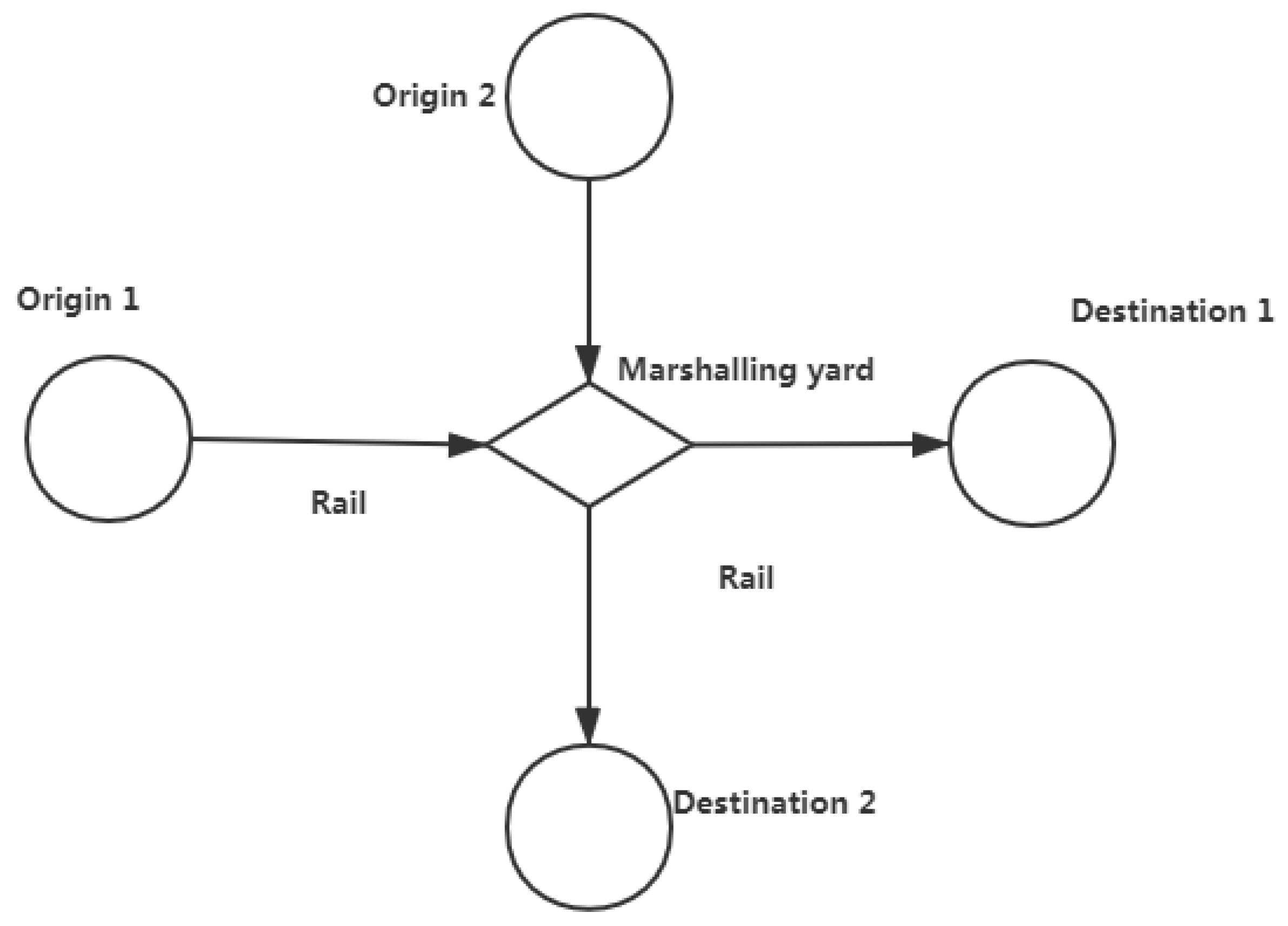
Figure 2.
Alternative Representations of Case Study Railway Network.
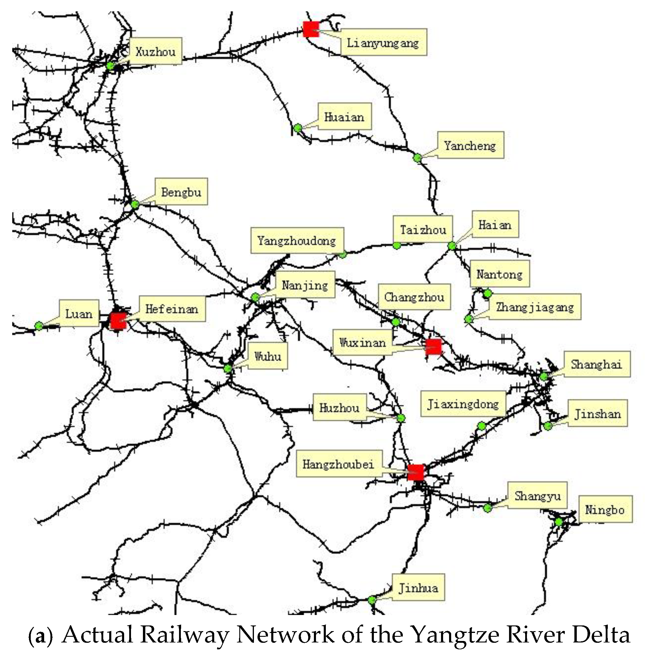
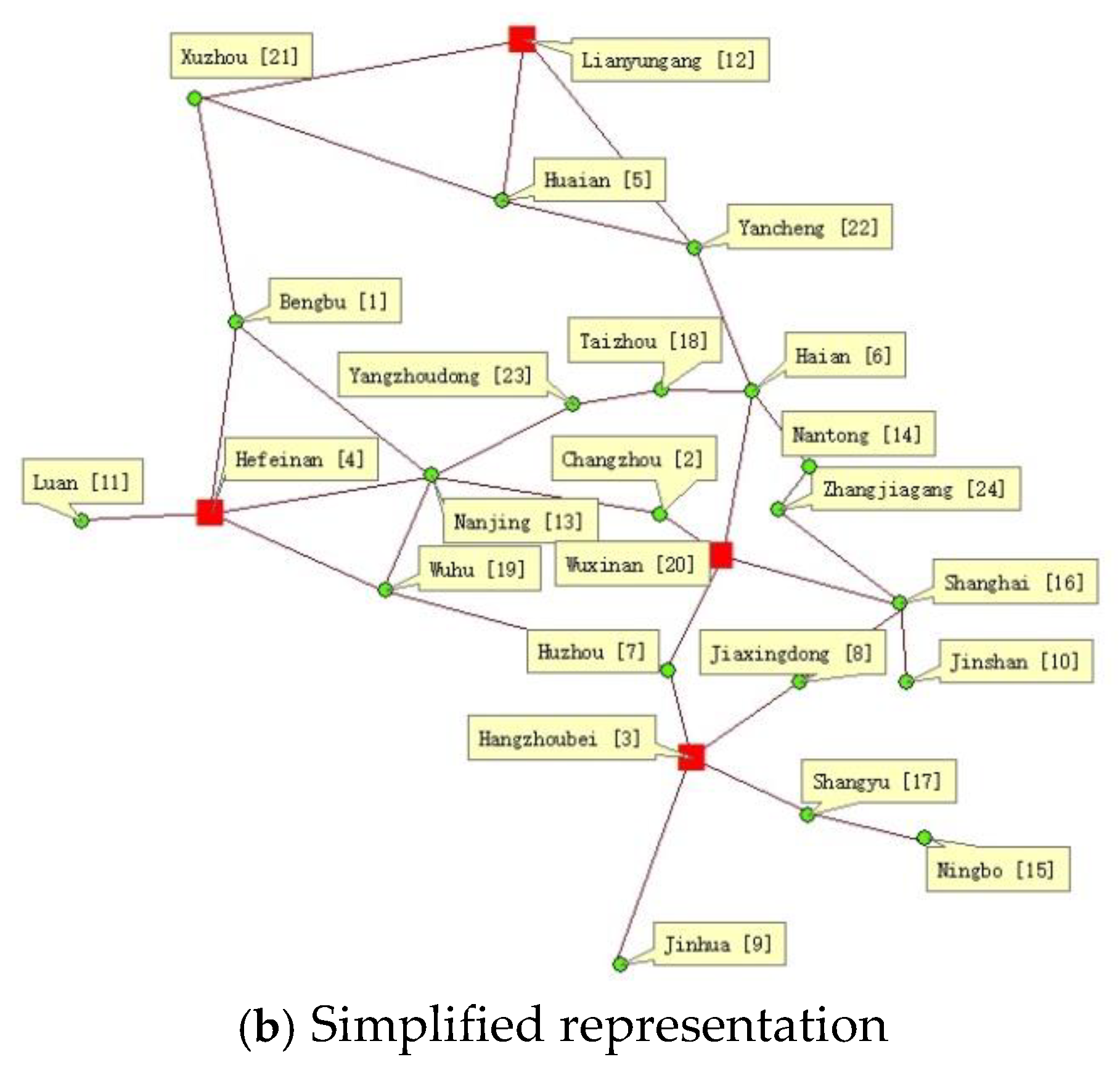
Figure 3.
Three-dimensional graph of the correlation between and route distance/average risk/Hazmat number.
Figure 3.
Three-dimensional graph of the correlation between and route distance/average risk/Hazmat number.
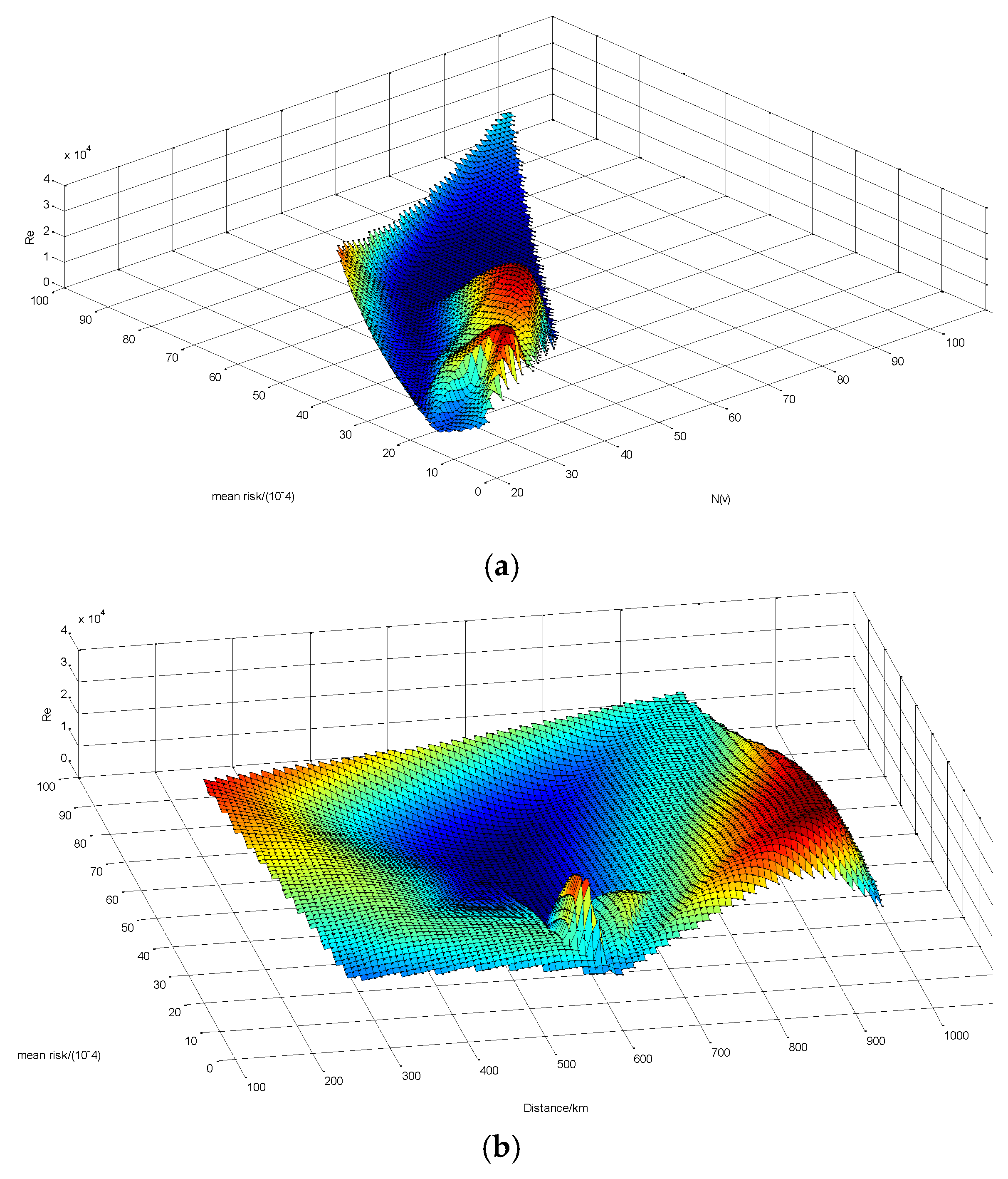
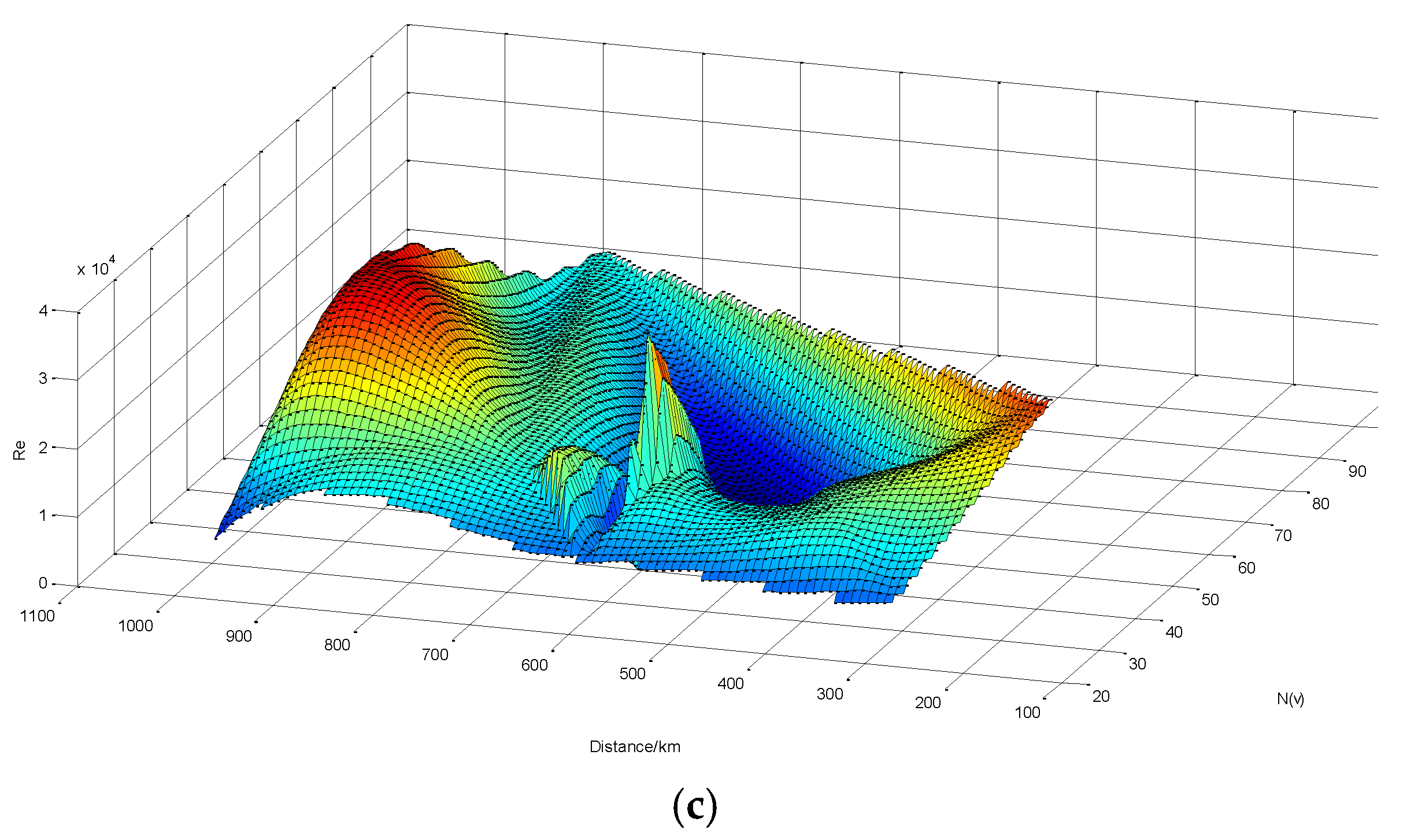
Figure 4.
CVaR and CVaRE value for the optimal route of two models in problem P.
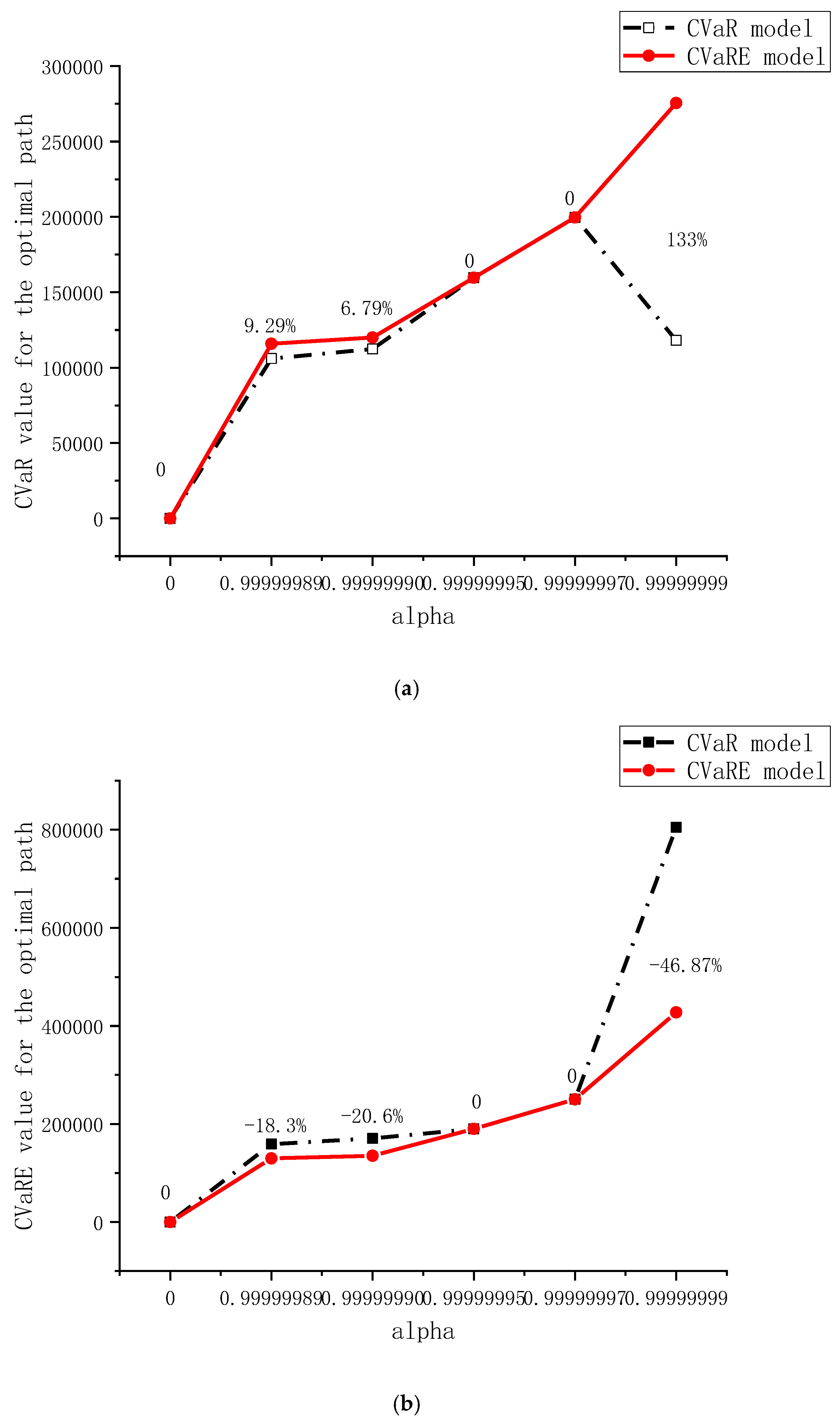

Table 1.
Optimal route based on CVaR of all O-D pairs and the corresponding value of y.
| Origin | Destination | N(v) | CVaR* | Route | |
| 1 | 12 | 30 | 20256.98 | [1,21,12] | 17 |
| 1 | 3 | 59 | 45842.12 | [1,4,19,7,3] | 23 |
| 4 | 14 | 39 | 49434.77 | [4,13,23,18,6,14] | 9 |
| 4 | 3 | 74 | 34381.59 | [4,19,7,3] | 23 |
| 4 | 12 | 54 | 30385.47 | [4,1,21,12] | |
| 5 | 14 | 23 | 27984.10 | [5,22,6,14] | 10 |
| 5 | 13 | 35 | 30385.47 | [5,21,1,13] | 17 |
| 7 | 1 | 25 | 31266.28 | [7,19,4,1] | 8 |
| 7 | 15 | 37 | 30606.14 | [7,3,17,15] | 11 |
| 9 | 13 | 31 | 44517.62 | [9,3,7,19,13] | 6 |
| 10 | 7 | 20 | 69064.39 | [10,16,8,3,7] | 1 |
| 11 | 14 | 24 | 46753.52 | [11,4,13,23,18,6,14] | 1 |
| 13 | 10 | 38 | 129906.74 | [13,19,7,3,8,16,10] | 23 |
| 15 | 3 | 54 | 18733.65 | [15,17,3] | 11 |
| 15 | 9 | 27 | 26859.05 | [15,17,3,9] | 6 |
| 15 | 19 | 40 | 45842.12 | [15,17,3,7,19] | 23 |
| 16 | 21 | 102 | 186583.81 | [16,8,3,7,19,4,1,21] | 25 |
| 16 | 13 | 54 | 115262.50 | [16,8,3,7,19,13] | 23 |
| 16 | 23 | 30 | 100118.54 | [16,8,3,7,19,13,23] | 9 |
| 16 | 9 | 31 | 64910.37 | [16,8,3,9] | 6 |
| 17 | 16 | 36 | 72276.81 | [17,3,8,16] | 11 |
| 18 | 20 | 48 | 43250.94 | [18,6,20] | 28 |
| 18 | 16 | 37 | 112363.00 | [18,6,14,24,16] | 21 |
| 20 | 11 | 30 | 38540.30 | [20,2,13,4,11] | 1 |
| 20 | 5 | 18 | 36919.47 | [20,6,22,5] | 3 |
| 22 | 24 | 12 | 25710.35 | [22,6,14,24] | 1 |
| 22 | 16 | 29 | 96069.21 | [22,6,14,24,16] | 10 |
| 24 | 10 | 39 | 78724.22 | [24,16,10] | 32 |
| 3 | 12 | 52 | 117998.97 | [3,7,19,4,1,21,12] | 23 |
Table 2.
The relationship between Risk equity() and other variables of different O-D pairs.
| O-D pair | N(v) | Distance(P) | ||
| (1,12) | 30 | 374 | 16906.03 | 25.36 |
| (1,3) | 59 | 553 | 0 | 34.35 |
| (4,14) | 39 | 550 | 15532.25 | 15.20 |
| (5,13) | 35 | 581 | 36197.46 | 15.85 |
| (9,13) | 31 | 587 | 14621.13 | 18.92 |
| (10,7) | 20 | 274 | 7886.06 | 15.21 |
| (11,14) | 24 | 606 | 8364.41 | 8.39 |
| (13,10) | 38 | 586 | 1880.56 | 40.45 |
| (16,13) | 54 | 544 | 0 | 63.04 |
| (16,21) | 102 | 878 | 14254.90 | 99.60 |
| (16,23) | 30 | 645 | 20646.36 | 22.06 |
| (18,16) | 37 | 709 | 15214.80 | 31.11 |
| (22,16) | 29 | 1002 | 2822.4 | 29.48 |
| (24,10) | 39 | 176 | 32237.57 | 61.71 |
| (3,12) | 52 | 927 | 34307.54 | 34.83 |
Table 3.
Comparison of VaR, CVaR, and CVaRE Models, when o-d is 18-16,N(v)=37.
| Risk-measure value | Route properties | |||||
| Model | Confidence level |
CVaRE* | CVaR* | VaR* | Number of arcs | Distance(km) |
| CVaR | 0 | 0.0189 | 0.0124 | 0 | 4 | 303 |
| 0.99999989 | 158818.48 | 106068.99 | 10755.56 | 4 | 303 | |
| 0.99999990 | 170387.44 | 112363.00 | 10807.08 | 4 | 303 | |
| 0.99999995 | 190079.78 | 159650.17 | 11460.53 | 7 | 709 | |
| 0.99999997 | 250355.35 | 199639.35 | 17737.43 | 7 | 709 | |
| 0.99999999 | 804905.68 | 118086.33 | 39362.11 | 3 | 297 | |
| CVaRE | 0 | 0.0189 | 0.0124 | 0 | 4 | 303 |
| 0.99999989 | 129759.72 | 115928.08 | 10755.56 | 7 | 709 | |
| 0.99999990 | 135202.78 | 119987.98 | 10807.08 | 7 | 709 | |
| 0.99999995 | 190079.78 | 159650.17 | 11460.53 | 7 | 709 | |
| 0.99999997 | 250355.35 | 199639.35 | 17737.43 | 7 | 709 | |
| 0.99999999 | 427682.78 | 275534.77 | 39362.11 | 7 | 709 | |
Table 4.
Sum optimal result of CVaR, CVaRE(different cases) and cost.
| Cost (CNY) | |||
| Direct transportation(base case) | 1721712.71 | 2234020.54 | 2349421.56 |
| Transfer transportation | 1848079.10 | 2777571.41 | 2361436.20 |
| Min cost(P) | 1906528.87 | 3014526.37 | 2169930.12 |
Disclaimer/Publisher’s Note: The statements, opinions and data contained in all publications are solely those of the individual author(s) and contributor(s) and not of MDPI and/or the editor(s). MDPI and/or the editor(s) disclaim responsibility for any injury to people or property resulting from any ideas, methods, instructions or products referred to in the content. |
© 2025 by the authors. Licensee MDPI, Basel, Switzerland. This article is an open access article distributed under the terms and conditions of the Creative Commons Attribution (CC BY) license (http://creativecommons.org/licenses/by/4.0/).
Copyright: This open access article is published under a Creative Commons CC BY 4.0 license, which permit the free download, distribution, and reuse, provided that the author and preprint are cited in any reuse.


