
Submitted:
23 January 2025
Posted:
24 January 2025
You are already at the latest version
Abstract
Degraded shock absorbers have a negative effect on the safety-critical driving dynamics of passenger cars. Oil and gas loss due to leaks at the shock absorber seals are the most common degradation mechanisms of vehicle shock absorbers. This paper presents degraded twin-tube shock absorber measurement results. Eight different twin-tube shock absorbers for passenger cars were modified and measured for this purpose. Based on this analysis, a semi-physical phenomenological model is derived which can represent the properties of a twin-tube shock absorber in the event of oil and gas loss. The model is parameterized based on quasi-static and dynamic harmonic measurements and is validated using harmonic and stochastic signals. The data analysis and a simulation study show that an oil loss of just 10 % can reduce the damping work performed by the shock absorber to 50 % compared to an intact shock absorber. Similarly, an oil loss of 50 % can lead to a reduction of the shock absorber work to zero. Oil foaming and cavitation must be taken into account when modeling the shock absorber characteristics in the event of oil and gas loss. It can be summarized that particularly long-lasting excitations at high shock absorber velocities, such as those that occur when driving on uneven roads, lead to a significant loss of damping work. This in turn leads to increased wheel load fluctuations and lower transmittable horizontal tire forces and unsteady driving behavior.
Keywords:
vehicle dynamics
; degraded vehicle components
; shock absorber modelling
; shock absorber testing
; shock absorber failure
; numerical simulation
1. Introduction
Driving tests show that degraded shock absorbers (SA) have a negative effect on the driving stability, the rollover stability and the braking distance of passanger cars [1,2,3,4,5,6,7,8,9,10,11]. Simulative studies also show the negative effects of degraded SAs on driving dynamics [6,12,13]. The degradation of technical components is defined as the reduction in technical performance due to wear and deterioration [14]. The degradation of SA means a reduction in the dissipation of vibration energy. Studies show that oil and gas loss due to seal failure is the most common cause of SA degradation [15,16]. Another cause of SA degradation is the SA valve defect, which will not be covered in this work [1].
Zwosta showed in a comprehensive study that oil and gas loss can significantly reduce the damping force of a twin-tube SA depending on the preconditioning and excitation of the SA [17]. The higher the maximum excitation velocity and the number of oscillations, the more significant the effect of oil loss on the work performed by the SA and therefore on the vibration energy dissipation. Although loss of the entire gas preload reduces the maximum damping force and damping work to a maximum of 10 %. However, a loss of 10 % oil volume in SAs can reduce damping work already by 30 %. An oil loss of 60 % (40 % oil level) can reduce the damping work to zero for high-amplitude and high-frequency excitations. Furthermore, the SA work is strongly dependent on the number of oscillations when oil is lost. On the basis of these observations, Zwosta concluded that the remaining oil in the degraded SA foams at higher velocities, thus greatly reducing the viscosity of the fluid flowing through the SA valves. In extensive tests, he was able to define a preconditioning method for measuring degraded SAs in the event of oil and gas loss. The limiting velocity for this foaming was determined to be 0.05 . He further concludes that the properties of a fluid damper in the event of oil and gas loss cannot be adequately represented by a scalar value or a modified force-velocity (F-v) curve.
Czop describes the collapse of the damping force at the beginning of the rebound and compression strokes on intact monotube and twin-tube SAs [18,19]. He describes similar effects to those of Zwosta, but sees the cause of these effects in the design of the SAs.
Hu shows the effect of oil loss on the behavior of a single tube fluid damper used in civil engineering [20]. He observed the collapse of the damping force as a function of the damper displacement and the oil level due to a gas flow instead of an oil flow through the SA valves. Furthermore, he shows the simultaneous flow of oil and gas through the valves in the transition area. He describes a model based on the investigations carried out. He considers excitation velocities of a maximum of 0.4 m/s.
Gao investigates the effect of cavitation on the behavior of a hydraulic yaw damper in the field of rail vehicle technology and presents a model to represent these effects [21]. The model calculates the phase proportions of the oil, the foam, the free gas and the gas dissolved in the oil as a function of the local pressure conditions in the damper and the fluid temperatures at every timestep of the simulation. In the damper model, many submodels of various damper components such as valves, orifices, and piston rods are used, which are addressed in separate publications [22,23,24].
The literature shows that no model of a degraded twin-tube passenger car SA has yet been developed that takes into account the loss of oil and gas. Similarly, no model of a degraded SA has yet been presented that is capable of modeling the relevant properties of a degraded SA with a small number of parameters and can be used in a full vehicle model. Gao describes a damper model that is well suited to model degradation mechanisms and, in particular, cavitation in fluid dampers. From the author’s point of view, the effort required for parameterization is very high to be used for large parameter studies in the field of automotive engineering. Zwosta presents extensive measurements on a modified twin-tube SA. The results of his investigations need to be confirmed for other vehicle SA.
This work is based on the research of Zwosta, Hu and Gao and presents a semi-physical phenomenological SA model that can represent the properties of degraded twin-tube SAs under oil and gas loss. Firstly, six different SAs were modified so that their oil and gas volumes can be altered. Various degradation states with the modified SAs were investigated, and a model was developed. In the next step, two more SAs were set to different degradation states in order to validate the developed model for realistic excitations. The model is to be used in full-vehicle models to further develop SA inspection methods and investigate the effect of degraded SAs on the safety-critical driving dynamics of passenger cars. The model requirements are the correct representation of the damping force for realistic SA excitation and different oil levels as well as a small number of parameters for use in full-vehicle models. The model is based on the standard modeling approach of passenger car SAs using the parallel connection of an F-v characteristic, a friction model, and a spring model. This model approach is extended by a semi-physical phenomenological degradation model and an adapted parameterization of the friction and spring model. This model is the first to represent the properties of degraded twin-tube passenger car SAs due to oil and gas loss and avoids extensive physical modeling of the fluid properties in order to ensure applicability in large parameter spaces in full-vehicle models.
2. Materials and Methods
A total of eight different twin-tube SAs were measured and analyzed on a single-axis hydropulser. The test rig is able to generate signals with a maximum frequency of 100 Hz. The maximum force of the test rig is 50 kN and the maximum deflection is 250 mm. The SAs examined are the front and rear axle SAs of four different passenger cars. Table 2 summarizes the SA information. To limit the SA temperature during measurements, the SAs were cooled with an air fan. At the start of each measurement, the SAs had an outer tube temperature of around 25 ° C. Due to dynamic excitations, the SA temperature rose by up to 5 K despite cooling. According to Hryciów, the energy dissipated by SA is reduced by approx. 2 % for a 5 K higher SA temperature [25,26]. The influence of temperature is not taken into account in the simulation model. However, the influence of 2 % should be taken into account when discussing the results. Figure 1 shows the SA test rig during the measurement of SA 7 with coordinate system.

Table 1.
Shock absorber information
| Shock absorber No. | Vehicle | Axle |
|---|---|---|
| 1 | Volkswagen Golf VI | Front |
| 2 | Volkswagen Golf VI | Rear |
| 3 | Volkswagen Passat B6 | Front |
| 4 | Volkswagen Passat B6 | Rear |
| 5 | Volkswagen Caddy III | Front |
| 6 | Volkswagen Caddy III | Rear |
| 7 | Volkswagen Passat B8 | Front |
| 8 | Volkswagen Passat B8 | Rear |
Initially, six of the eight twin-tube SAs (SA 1 to SA 6) were fitted with external valves so that their gas pressure and oil volume could be varied. The SAs were sawn apart, modified, and welded back together. Before welding the SA halves, the geometry of the SAs was determined, which is necessary for model parameterization. To validate the modified SAs, their F-v characteristics were recorded and compared before and after the modification. The SAs after modification were provided with the complete oil volume and the original gas pressure for this purpose. Figure 2 shows one of the modified SAs. Figure 3 shows the F-v characteristics of SA 1 to SA 6 before and after the modification in the intact state. The figure also shows the F-v characteristics of SA 7 and SA 8 in the intact state.
The properties of all eight SAs were examined in the event of oil and gas loss. In addition to the intact state, each SA was set to two different degradation states, which are defined by a percentage of the oil volume. The gas pressure was reduced to 0 for these degradation states, as a complete loss of gas pressure can be assumed with a greater loss of oil volume. In order to investigate the properties of the SAs 1 to 6 in the event of oil and gas loss, they were each measured with eight different velocity blocks, each consisting of 19 sinusoidal oscillations. The amplitudes of these oscillations correspond each to 90 % of the maximum stroke of the SAs. SAs 7 and 8 were measured with 17 different velocity blocks, each with 19 oscillations and an amplitude of 45 mm. Before each velocity block of the 19 sinusoidal oscillations, 6 sinusoidal oscillations with the same amplitude and a maximum velocity of 0.05 were placed as preconditioning. After each measured velocity, the SA stood still for 180 s. The preconditioning method was derived from the results of Zwosta [17]. Furthermore, quasi-static friction measurements were carried out at a velocity of 1 mm/s.
To achieve the specific damping states of SA 7 and 8, the two SAs were each drilled, the gas and oil drained and welded back together. SAs 7 and 8 were measured in each state with the same measurement program before the next damping state was established. The oil quantities removed were documented for each condition and deviate slightly from the target values of 60 % and 40 % oil level of the total oil quantity. Table 2 summarizes the actual oil volumes of all SAs and SA states.
Based on the analysis carried out on the eight different SAs, a model was developed that can represent the properties of the degraded SAs. To validate the model, SAs 7 and 8 were also measured with ten different stochastic excitations. These signals correspond to the SA deflections of SA 7 and 8 during driving maneuvers performed with the Volkswagen Passat B8 test vehicle. Figure 6 shows the potentiometer for measuring the stroke of the front axle SA of the test vehicle. Table 3 lists the ten driving maneuvers for measuring the stochastic SA signals, besides the quasi-static and harmonic signals. Figure 4 and Figure 5 show the measured displacement excitations of the stochastic signals for SA 7 over time. The stochastic signals are composed of a slow bump crossing, different cleat crossings, uneven road drives, and braked uneven road drives. The slow bump crossing is a dynamic SA inspection method [27,28]. The uneven road drives and the braked uneven road drives validate the SA model for the simulation of safety-critical driving maneuvers within a full vehicle model. The uneven road is assigned to road class D. Each stochastic signal was preceded by six oscillations for preconditioning. The quasi-static measurements and the harmonic measurements are used to analyze the SA properties and to parameterize the model, while the stochastic signals are later used for model validation.
3. Results
3.1. Data Analysis
The force generated by a twin-tube SA can be categorized into three parts: gas force, friction force, and fluid force. Figure 7 shows the force-displacement (F-s) diagram of the SA 7 for the quasi-static friction measurements. The friction force and the gas force were measured with ramp signals at a constant velocity of 1 mm/s. The figure shows that the increase in the curves for the intact configuration with gas preload is significantly higher than the increases in the degraded states without gas preload, which is close to zero. It can also be seen that the measurements show an offset. This offset can be explained by the fact that the test setup on the single-axis test rig is not always free of lateral forces and amounts to a few Newtons. A slight tension of the SA leads to an offset and a slightly different friction force.
Figure 8 shows the F-s characteristics of all SAs with an oil level of nearly 40 % and 100 % of the harmonic measurements with a maximum velocity of 0.05 . The figure shows 19 oscillations for each condition. It can be seen that all 19 oscillations of a condition are well superimposed. For the degraded state, it can also be seen that the damping forces in the rebound and compression stages are initially very low and increase sharply from a certain point of deflection. Furthermore, it can be seen that the forces of the intact SAs are not reached after this increase. The relative proportion of the forces in relation to the intact SAs is different for each SA and is therefore SA-specific. For measurements with SA velocities greater than 0.05 , it was found that the F-s curves of the 19 consecutive oscillations do not overlap. Figure 9 shows the F-s characteristics of all SAs for an oil level of nearly 40 % and 100 % respectively for the 19 sinusoidal oscillations with a maximum velocity of 1 .
Figure 10 graphically represents the F-s diagram of the 19 sinusoidal oscillations with a maximum SA velocity of 1 for SA 1 with an oil level of 40 %. In the figure, the individual oscillations are separated from each other by color. The figure shows that the damping force is initially very low in the rebound and compression stages and increases dramatically with deflection, as can also be seen in Figure 8 for low SA velocities. However, the figure also shows that the increase in force in the rebound and compression stages occurs later for an increasing number of oscillations.
Furthermore, Figure 11 graphically represents the work performed by all SAs with 40 % oil level for the 19 sinusoidal oscillations with all the measured maximum SA velocities. The diagrams show that the work performed per oscillation remains constant for low velocities. For higher velocities, it can be seen that the work performed per oscillation sometimes decreases very sharply as a function of the number of oscillations. For all front axle SAs, it can be observed that the work performed per oscillation for the highest maximum velocity of 1.6 decreases to such an extent that less work is performed per oscillation than for significantly lower maximum velocities. This is less noticeable for the rear axle SAs tested. The observed decrease in damping work performed per oscillation as a function of the number of oscillations for higher excitation velocities thus appears to be SA-dependent. Since similar behavior can be observed for front and rear axle SAs, it can be assumed that this property is particularly influenced by the geometry of the SAs and the flow conditions in the SA, since the front and rear axle SAs dimensions are slightly different.
3.2. Shock Absorber Model
The SA model is intended to be used in full-vehicle models to simulate SA inspection methods and safety-relevant driving maneuvers. The model is derived on the basis of the measurements shown. The model is parameterized using the quasi-static and harmonic measurements. The model is validated by comparing the measured and simulated harmonic excitations of all SAs. In addition, the measured and simulated damping forces and the damping work performed for stochastic excitations for SAs 7 and 8 are compared.
A parallel arrangement of a spring, a Dahl- friction model and a F-v characteristic curve is used to represent the intact SA [29,30]. The oil and gas loss in the SA affects all three parts. The models for calculating the gas force and the friction force remain unchanged. However, the parameters are adjusted according to the degradation condition. The damping force of fluid friction is multiplied by a degradation factor at each time step of the numerical simulation. This factor is calculated using a degradation model that can calculate the reduction in damping force in relation to the potential damping force of the intact SA. Formula (1) represents the calculation of the total damping force.
Table 4.
Formula symbol definition
| Formula Symbol | Description |
| Simulation timestep | |
| z | Piston rod displacement; stroke |
| Piston rod velocity | |
| Area of the piston valve to the rebound chamber | |
| Area of the piston valve to the compression chamber | |
| Volume of the rebound chamber | |
| Volume of the compression chamber | |
| Volume of the reserve chamber | |
| Preasure in rebound chamber | |
| Preasure in compression chamber | |
| Total shock absorber force | |
| Shock absorber gas force | |
| Shock absorber friction force | |
| Shock absorber fluid friction force | |
| Degradation factor | |
| Gas spring stiffness | |
| Slope of the hysteresis loop | |
| saturated quasi-static friction force | |
| Exponent of the hysteresis friction gradient | |
| F-v-characteristic | |
| Volume flow rate | |
| Relative oil volume flow | |
| Relative oil volume flow change | |
| Cavitation treshold velocity | |
| Cavitation factor | |
| Total measured shock absorber force | |
| Total simulated shock absorber force | |
| Total measured shock absorber work | |
| Total simulated shock absorber work |
In case of gas loss, the gas pressure and therefore the considered spring force of the SA is reduced. In case of oil loss, the gas volume also expands and the gas pressure in the SA is reduced. The spring force of the SA is defined by the increase in the F-s characteristics of the quasi-static measurements. In case of oil loss, the friction force of the SA increases [31]. According to Stribeck, the friction force also depends on the velocity [32]. A Dahl-friction model is therefore used, which is scaled via the velocity with a SA-specific Stribeck curve. The saturated Dahl-friction is determined with the quasi-static friction measurements and corresponds to half the hysteresis width of these measurements. The velocity dependence of the friction force is taken from Deubel and is shown in Figure 12. The parameter defines the velocity dependence of the friction force. Equation (2) describes the calculation of the friction force in the SA model.
The loss of oil and gas affects the fluid force of the SA the most. The fluid force of the intact SA is calculated using a friction-reduced F-v curve. This characteristic curve is determined from the harmonic measurements of the intact SA at a displacement of 0 mm. The F-v curves of the SAs are shown in Figure 3. The loss of oil and gas reduces the potential fluid force of the SA depending on its geometry, displacement, and hydraulic characteristics. To represent this reduction in force, the calculated potential damping force of the F-v curve is modeled using a degradation model, which is presented here. Figure 13 shows the twin-tube passenger car SA. The force between the connection points of the SA is caused by the pressure difference between the top and bottom of the piston valve (PV), the different sizes of the top and bottom of the PV and by friction forces between the piston rod (PR) and seal (OS) as well as between the PV and the inner tube wall of the SA (IT). Equation (3) shows the calculation of the SA force calculated on the basis of the pressure and area difference in the PV.
The pressures on the top and bottom of the PV can be calculated from the flow of the oil and the gas pressure in the reserve chamber (RC). When the PR and the PV move, the SA oil flows through the PV and the bottom valve (BV) to equalize the pressure in the working chambers and . The oil flow through the valves causes fluid friction, which is largely responsible for the force of the twin-tube SA. This force is only generated when the oil flows through the valves. If gas flows through the valves, this force is not generated.
Figure 8 shows that the fluid force of the degraded SA depends on the deflection of the SA. The figure suggests that the respective increase in force during rebound and compression is caused by an oil flow through the SA valves, which did not take place before. It can be assumed that the PV is immersed in a volume of oil at this point. The figure also shows that the force of the intact condition is not reached after the increase in force. The force achieved after the force increase is different for each SA in relation to the force of the intact SA. Therefore, it is assumed that this difference is caused by the volume flow of oil through the two SA valves. To calculate these forces, the degradation model calculates the volumes of the individual working chambers and the volumes of the media in the working chambers at each time step in the numerical simulation.
The parameters and each describe the relative flow of oil volume through a SA valve in relation to the oil volume flow through a SA valve when the SA is intact (equations (14) and (15)). If the parameters and are equal to one, the oil volume flow through the valves corresponds to the oil volume flow through the valves when the SA is intact (equations (17) and (19)). It is assumed that the oil performs the full potential work on the valves. If a volume flow of gas or foam is detected through the valves, the work performed on the valves is relatively reduced. If only gas flows through a valve, no work is performed and the parameters and become zero (formulae (16) and (18)). In order to calculate the volume flows of the various media through the valves and to correctly reduce the potential damping force, case distinctions are made. It is assumed that in the rebound stage, the damping force is generated exclusively by the flow of oil through the PV, whereas in the compression stroke the damping force is generated by the flow of oil through the PV and BV [33].
For higher SA velocities, it can be observed in Figure 11 that the damping force decreases with increasing number of oscillations. It can be observed that the damping force in the rebound and compression stages builds up later during the 19th oscillation than during the first oscillation.
Gao and Czop present models that describe the reduction in SA force as a result of cavitation [18,19,21]. These models calculate the dissolving of gas from the SA oil and the foaming of the SA oil with gas. The model presented here also calculates the oil, gas, and foam volume fraction in the individual working chambers at each timestep according to Figure 13. For simplified later application in full-vehicle models, the model presented here calculates the volume fractions using a phenomenological approach. Starting from an initial state, the change in the volume of the rebound working chamber (equation (6)) and the compression working chamber (equation (7)) is calculated when the PR is displaced. Additional oil or oil foam volume loss through the upper SA seal is neglected (equation (13)). The volume change of the compression working chamber (equation (9)) takes place through the PV (equation (11)) and the BV (equation (12)). Only the volume of oil and foam is taken into account in the reserve chamber. The volume change of oil and foam in the reserve chamber only takes place through the BV (equation (10)). Figure 14 shows the volume of the compression chamber and the corresponding volume fractions of oil, gas and oil foam of SA 1 as an example for a harmonic excitation with an amplitude of 45 mm. It can be seen that the oil in the SA is not sufficient to completely fill the compression chamber to its maximum volume. When the working chamber is at maximum volume, it also contains a gas volume and an oil foam volume.
The initial state of the SA is defined before starting the simulation. For this purpose, the oil volumes in all three working chambers are defined and the displacement of the SA is adopted at the start of the measurement. During the simulation, a distinction is made between the SA states. A distinction is made as to whether the SA is in rebound or compression, whether the velocity of the SA is greater or less than 0.05 m/s and whether there is only oil, only gas, oil and gas, oil and foam or oil, gas and foam in the individual working chambers of the SA. The damping force component at both SA valves is calculated for the compression stage. Therefore, all working chambers are relevant. If the SA is in the rebound stroke, only the oil flow through the PV is taken into account.
If the velocity of the SA displacement is less than 0.05 , it is assumed that the oil does not foam and there is no cavitation. This threshold velocity was determined by Zwosta and could also be observed for all measurements presented here and is shown in Figure 8 [17]. Without foam in the working chambers, gas can flow through the valves first and then oil, or only oil if there is no gas volume in the working chamber. If only gas flows through the SA valves, the fluid force component is reduced to 0 N for the valve in question. If only oil flows through the valve, the full potential damping force is applied.
For simplified calculation of the volume flows through the SA valves, the volumes of all working chambers and the oil volume in the SA must be known. For the parameterization of the model, all SAs were disassembled. Figure 15 and Table 5 show the relevant dimensions of the SAs.
Hu found that oil and gas can also flow through the SA valves at the same time [20]. This process can also be seen in Figure 8. Therefore, the parameter X is introduced, which describes for each SA valve the proportion of oil that flows through a valve simultaneously with a proportion of gas.
The leakage factor is introduced, which defines the proportion of oil that flows from one working chamber to another but does not generate a damping force. The parameters X and can each range from 0 to 1. Figure 16 shows the influence of both parameters on the calculation of the force in the rebound stroke in the F-s diagram. The change in the relative flow of oil volume through PV is calculated using the leakage factor and the parameter (equation (22)). Equations (23) to (25) describe the calculation of the damping force in the rebound stroke for low velocities. The Table 6 and Table 7 list and explain all parameters of the degradation model.
During compression stroke, SA oil can flow through both the PV and the BV. The parameter defines the proportion of oil flow through the PV in the total oil flow out of the compression chamber (). This parameter also varies between 0 and 1. The complement part to 100 % of the oil flow flows through the BV (equation (26)). If there is only gas in , then only gas flows through the PV. Therefore, no fluid force is generated. If oil and gas are in at the same time, oil flows through the BV into the reserve chamber and gas flows through the PV into the rebound chamber. The volume change in the compression chamber is described by equation (26). The parameter defines the proportion of oil in the volume flow from through the BV. If is completely filled with oil and there is gas in the rebound chamber, the venting of the rebound chamber also results in a state with a proportional damping force. Oil flows from to both the rebound chamber () and the reserve chamber (). In this case, the proportion of volume flow through the BV in the volume change of depends on parameter , which can range from zero to one.
Due to the venting of the rebound working chamber, the oil volume flow through the PV can be larger than in the intact condition. Therefore, the parameter is introduced. This parameter can also range from zero to one and describes the proportion of the damping force due to the increased oil volume flow through the PV. This results in the following calculation of the proportional damping force in relation to the potential damping force:
The measurement data show that the damping force decreases continuously over the number of oscillations when the SA is excited at high velocities and contains less than oil. This behavior can also be seen in Figure 10 and Figure 11. This observation is explained by the foaming of the oil and cavitation in the degraded SA. Foam generation is assumed to be maximized when gas flows through oil. Other processes that could lead to foam generation, such as the flow of oil through a valve or the further foaming of existing foam, are neglected. In addition, the foam is generated without a time delay. When foam is generated, the foam volume corresponds to the sum of the proportions of air volume and oil volume. Overall, the sum of all volumes in the working chambers remains constant. The foam decomposition occurs only during rebound if the rebound working chamber is partially filled with foam and oil. The dissolution of foam during standstill is neglected due to the air separation capacity of the oil.
If gas flows through an oil volume at a SA velocity of more than 0.05 m/s, foam is generated in the working chamber, which initially contains oil. Foam generation is treated separately for BV and PV and is characterized by the respective parameters S and . S and can range from 0 to 1. S specifies the proportion of the gas volume flow that is converted to foam. specifies the oil proportion of the foam. A value of one means that the foam consists equally of gas and oil. If all conditions are met, it is checked whether there is enough oil () in the working chamber of the possible foam generation for complete foam generation in line with the parameters (equation (30)).
The change in foam volume due to foam formation results from the sum of the proportions that are converted from the gas volume flow and the existing oil volume (equation (31)).
The oil proportion of the generated foam is determined accordingly by the parameter (equation (34)).
If there is not enough oil, it is completely converted into foam. This means that only part of the actual foam volume can be generated. If further foam is formed in a working chamber in which foam is already present, or if additional foam flows in, mixing occurs. It is possible that the respective foams and have different oil proportions and . Consequently, the oil proportion of the total mixed foam must be recalculated with the individual volume proportions as weighting in equation (35).
Foam can decompose during rebound. To characterize the proportional damping force at certain foam volume flows through the valves, an exponential approach is used with the parameter B as a factor, which ranges from zero to one, and the parameter E as an exponent (equation (36)).
The factor B indicates whether the foam generally behaves more like a gas, with a value of zero, or like oil, with a value of one. Exponent E describes the relationship between the proportion of oil in the foam and the proportionate damping force. A value of one results in a linear relationship and as the exponent increases, the proportional damping force for a certain proportion of oil decreases due to a non-linear, progressive relationship (Figure 18).
The resulting damping force therefore results from the foam properties in combination with the described calculation of the volume flows of oil, gas, and foam through the SA valves. An increase in the parameter S leads to increased foaming and therefore to a decrease in the volume of pure gas. A reduction in the parameter leads to a reduction in the proportionate damping force of the foam. This effect is intensified by reducing the parameter B and increasing the parameter E. Equations (37) to (39) show the calculation of the degradation coefficient for high stroke velocities during the rebound stroke.
The foaming of the oil is not sufficient to explain the significant decrease in damping force and therefore the work performed by the SA at high excitation velocities (Figure 10 and Figure 11). Like other mineral oils, the oil in vehicle SAs dissolves gas [34]. In steam cavitation, gas is released in the oil when the local pressure falls below the saturated vapor pressure. Mineral oil dissolves a maximum of 9.3 % - 11.3 % of its own volume as gas at normal ambient pressure and temperature. If the local pressure of the oil falls below the saturated vapor pressure, it takes between 3.6 and 7.6 s for half of this gas volume to be released. If the pressure does not fall below this value, it takes 6.1 to 10.2 s until half of the gas is dissolved.
At high excitation velocities, a significant pressure decrease can occur in the SA valves, resulting in the release of gas due to cavitation [35]. Therefore, it is assumed that the sharp decrease in SA work in Figure 10 and Figure 11 at high excitation velocities is a result of cavitation. To model this effect, it is assumed that the oil flowing through a valve is converted into gas above a SA-specific threshold velocity . Equations (40) and (41) illustrate this relationship. It is assumed that cavitation occurs only in the PV. A cavitation parameter is introduced for each of the compression and rebound directions.
The parameters in Table 6, Table 7 and Table 8 are SA-specific. They are optimized on the harmonic measurements of the SAs with the oil levels 40 % and 60 % by means of particle swarm optimization. It is assumed that these 14 parameters are the same for all oil levels of a SA. The parameters are optimized in two steps. In the first step, the five parameters for the basic model (Table 6) are optimized with the harmonic measurements up to and including a maximum SA velocity of 0.5 . In the second step, the six parameters of the foaming model (Table 7) and the three parameters of the cavitation model (Table 8) are optimized using the harmonic measurements with a maximum SA velocity of 1.6 . The sum of the Root-Mean-Square-Errors (RMSE) of the damping forces and the damping work performed from measurement and simulation is used as the optimization function. The formula (42) represents the calculation of the optimization function with the data points i and the length of the signal n.
3.3. Validation
To evaluate the quality of the model, the measured data is compared with the simulated data. The input values of the model correspond to the measured displacement excitations. The work and force performed by the SAs is used as the evaluation criterion. Figure 19, Figure 20, Figure 21, Figure 22, Figure 23, Figure 24, Figure 25 and Figure 26 show the comparison of the measured and simulated work of one oscillation of the harmonic excitations for the eight SAs for all velocities and oil levels. The figures show the work performed for the first and 19th oscillation. These diagrams show that the work performed decreases as the oil level decreases. It can also be seen that the work performed in the 19th oscillation at high excitation velocities is less than the work performed in the first oscillation. As shown in Figure 11, it can also be seen that the damping work performed for a harmonic excitation with a maximum velocity of 1.6 is partially lower than the work performed for lower velocities. The comparison between measurements and simulations shows that the simulation model is able to reproduce the measurement data.
Figure 27 shows the F-s diagram of the simulated and measured damping force for SA 1 with 60 % oil level for one harmonic oscillation with a maximum velocity of 0.08 . The figure shows that the qualitative behavior of the force at lower excitation velocities can be reproduced with the simulation model. The force steps can be explained by the different types of fluid flows. As soon as oil begins to flow through a valve, the damping force increases. This process is often smoother in reality. The build-up of damping force is smoother, especially at higher velocities.
The model is able to represent the decrease in damping force due to oil foaming at high excitation velocities. Figure 28 shows the F-s diagram of SA 1 with an oil level of 40 % for 19 harmonic oscillations with a maximum excitation velocity of 1.6 . The figure shows the 19 measurement oscillations in blue and the first and 19th simulated oscillations in green and red, respectively. The figure shows that the damping force continues to decrease as the number of oscillations increases. The simulation model is also able to reproduce this effect qualitatively with the foaming model and the cavitation model.
In addition to validating the model on the harmonic measurements, the parameterized models for SAs 7 and 8 were validated on the stochastic signals measured in the road tests. Table 3 lists all the signals measured on the SA test rig. The slow bump crossing (measurement 3) is a dynamic SA inspection method. To evaluate the simulation quality of the SA model, the Figure 29 and Figure 30 show the measured and simulated damping forces of both SAs for all investigated conditions. The figures show that the SA model is able to reproduce the damping forces well in the case of excitations caused by the slow bump crossing.
The SA model will also be used to investigate the effect of degraded SAs in the event of oil and gas loss on safety-critical driving dynamics maneuvers. The model was therefore additionally validated using the stochastic excitation signals 4 to 12 from Table 3. Figure 31 and Figure 32 show the percentage of damping work performed by the measurements and simulations in relation to the intact state for the various stochastic excitations. The figures show that the simulation model provides a good representation of the work performed by the SA.
3.4. Simulation Study
In addition to Figure 26, Figure 33 shows the work performed by SA 8 for 60 % oil level for the first and 19th oscillation of the harmonic measurements. The figure compares the measurement results with four different model variants. Model variant 1 is a scalar factor that corresponds to the oil level and is multiplied by the potential SA force of the intact SA. Model variant 2 is the basic model without foaming and cavitation. Model variant 3 is the basic model with foaming model. Model variant 4 is the complete degradation model presented here.
The figure shows that model variants 2 to 4 can reproduce the work performed during the first oscillation with a maximum error of 10 %. A simple scalar factor (model variant 1) underestimates the work performed by the first harmonic oscillation by 25 % in some cases. When analyzing the 19th oscillation, it can be seen that only model variant 4, which takes cavitation into account, is able to reproduce the decrease in damping work performed for a maximum excitation velocity of 1.6 . All other model variants overestimate the damping work performed for these excitations. This analysis leads to the conclusion that the use of a simple scalar factor, which corresponds to the oil level of the SA, is not sufficient to represent the effect of oil and gas loss in twin-tube SAs. A scalar factor underestimates the work performed by the SA for excitations at low velocities and for excitations at high velocities of more than 1 and a low number of oscillations. In the case of continuous excitation with excitation velocities of more than 1 , a scalar factor overestimates the work performed by the SA. As a result, a more complex SA model that takes cavitation into account is required to estimate the effect of degraded SAs on the safety of passenger cars, as otherwise there is a risk of underestimating the effect of degradation. A SA inspection method based on a slow bump crossing excites the SAs only briefly at high excitation velocities. Simple SA models thus overestimate the effect of degradation and simplify the supposed detection of a degradation state.
Finally, Figure 34 graphically shows the simulated work performed by SA 8 for the first and 19th oscillation of the harmonic measurements for oil levels from 0 to 100 %. The figure shows that even an oil loss of 10 % (oil level 90 %) reduces the damping work performed at excitation velocities above 0.5 from the first oscillation onwards. Furthermore, even at an oil level of 50 % for the 19th oscillation, the damping work performed is reduced to almost zero at an excitation velocity of 1.6 , while 65 % of the work of the intact SA is still performed during the first oscillation. This leads to the conclusion that even a minor oil loss in a vehicle SA leads to a significant reduction in damping work performed, which in turn means a safety risk for the vehicle.
4. Discussion
For the first time, this work presents extensive measurement results on the effect of oil and gas loss on the characteristics of various twin-tube SAs for passenger cars. The investigations are based on the findings of Zwosta, who carried out similar investigations for a single SA [17]. The results presented here confirm Zwosta’s observations that the loss of damping force and therefore the damping work performed by a twin-tube SA due to oil and gas loss are initially dependent on the type of excitation. Particularly long-lasting excitations with high velocities of more than 1 m/s lead to a very strong decrease in the damping forces and thus to a decrease in the damping work performed (Figure 11). These properties are SA-specific. SAs of similar design and dimensions have also been observed to show similar degradation behavior (Figure 11, Table 5). For the first time, this work presents a model that can represent the characteristics of a twin-tube SA with oil and gas loss. The model is a semi-physical phenomenological model, which on the one hand uses the SA dimensions, the oil volume, and the SA properties in the intact state as physically motivated variables, and on the other hand uses parameters that phenomenologically represent the valve properties of the SAs as well as their foaming and cavitation properties. The model was validated using harmonic and stochastic measurements of eight different SAs.
The differences between the simulations and the measurements result mainly from the specific fluid flows between the individual working chambers. Figure 27 and Figure 28 show that the model represents fluid flows qualitatively, but that inaccuracies occur. These inaccuracies are due to the non-linear behavior of the fluids and the macroscopic phenomenological model approach. More complex physical modeling approaches, such as those presented by Gao are required to represent the fluid properties more precisely, including the cavitation processes [21]. The modeling presented here is well suited to investigate the effect of degraded SAs on the full vehicle characteristics, as all the main effects are represented. An additional major advantage of the described phenomenological modeling is the simple parameterization compared to the physical approaches. Furthermore, the degradation model and its parameterizations can be applied to any F-v characteristics, which are used in full vehicle models for SA modeling. A simulation study of various model approaches shows that it is particularly necessary to take cavitation into account in order to reproduce the properties of degraded SAs in the case of excitations with sustained high velocities. In practice, SA excitations with persistently high SA velocities occur particularly when driving over uneven roads (Figure 5). To investigate the effect of degraded SAs on the safety-critical driving dynamics of passenger cars, it is particularly necessary to take cavitation in the SAs into account, as otherwise the effect of degraded SAs can be underestimated (Figure 5). At the same time, simple degradation models, such as a simple scalar factor, underestimate the damping work performed for one-time excitations, such as a speed bump crossing (Figure 5). This means that simple degradation models overestimate the effect of degraded SAs in the development of dynamic SA inspection methods and at the same time underestimate the effect on safety-critical driving dynamics. Another simulation study examines the effect of the oil level on the work performed by the SA. This simulation study shows that an oil level between 40 % and 60 % represents a transition range of the damping work performed. Although the work performed by SA is still more than 50 % at an oil level of 60 %, the work performed by the SA drops to almost zero at an oil level of 40 %. The model of a degraded SA presented here is therefore able to model the effect of oil and gas loss on the characteristics of twin-tube SAs. This model can therefore be used in the future to investigate the effect of degraded SAs on the driving dynamics of passenger cars. The great advantage of the model is that investigations can be carried out in a large parameter space, as the model is based on the characteristics of the intact SAs, in the form of the F-v characteristic curve, and the number of other parameters is limited, or existing data sets can be applied to other SAs.
5. Conclusions
This work analyzes the effect of oil and gas loss on the characteristics of twin-tube SAs in passenger cars and presents a semi-physical phenomenological model. For property analysis, eight different twin-tube shock absorbers from four different vehicles were brought to different states of degradation and extensively measured. Data analysis shows that higher excitation velocities in the degraded SA lead to an increased reduction in the damping work as a function of the number of oscillations. Based on the data analysis, a semi-physical phenomenological model is developed, which calculates the fluid flow within the SA at each simulation time step. The degradation model reduces the potential damping force on the basis of a case distinction as to whether oil, gas or oil foam flows through the SA valves. A cavitation model estimates the release of gas in SA oil at high excitation velocities. The validation of the model shows that considering cavitation is necessary to represent the damping characteristics for high excitation velocities. A simulation study showed that simpler models, which in particular do not take cavitation in degraded SAs into account, run the risk of overestimating the effect of degradation for short-duration SA excitations or long-duration SA excitations with low velocities, while they underestimate the effect of degradation for long-duration SA excitations with high velocities. As a result, simulation studies that aim to investigate the effect of degraded SAs due to oil and gas loss on safety-critical driving dynamics underestimate the effect of degradation. However, simulation studies with simple SA models overestimate the effect of degradation for short-term SA excitations, as they occur in various SA inspection methods, such as speed bump crossing. To increase road safety, future studies should be carried out on the effect of degraded vehicle SAs on the safety-critical driving dynamics of passenger cars, taking into account the characteristics of degraded SAs described here. It can be assumed that previous studies underestimate the effect of degraded SAs on driving dynamics. At the same time, easy-to-perform SA inspection methods that can detect vehicles with degraded SAs at an early stage should be developed.
Author Contributions
Conceptualization, T.S. and T.Z.; methodology, T.S. and T.Z.; software, T.S. and T.Z.; validation, T.S. and T.Z.; formal analysis, T.S.; investigation, T.S. and T.Z.; resources, T.S., T.Z. and G.P.; data curation, T.S. and T.Z.; writing—original draft preparation, T.S.; writing—review and editing, T.S.; visualization, T.S.; supervision, G.P.; project administration, T.S. and T.Z.; funding acquisition, G.P. All authors have read and agreed to the published version of the manuscript.
Funding
This research received no external funding.
Data Availability Statement
The data presented in this study are available on request from the corresponding author due to privacy restrictions.
Acknowledgments
The authors would like to express sincere gratitude to Fahrzeugsystemdaten GmbH for providing the test vehicle. The Article Processing Charge (APC) were funded by the joint publication funds of the TU Dresden, including Carl Gustav Carus Faculty of Medicine, and the SLUB Dresden as well as the Open Access Publication Funding of the DFG.
Conflicts of Interest
The authors declare no conflicts of interest.
Abbreviations
The following abbreviations are used in this manuscript:
| SA | Shock absorber |
| F-v | Force-velocity |
| F-s | Force-displacement |
| PV | Piston valve |
| BV | Bottom valve |
| PR | Piston rod |
| OS | Shock absorber seal |
| IT | Inner tube wall of the shock absorber |
References
- Wegener, D.B. Prüfverfahren für Schwingungsdämpfer im Fahrzeug. PhD thesis, RWTH Aachen University, 2020. [CrossRef]
- Rompe, K. TÜV Kraftfahrt GmbH Köln: Warum muss die Wirksamkeit der Stoßdämpfer regelmäßig überprüft werden? TÜ 1998, 39. [Google Scholar]
- Laermann, F.J. Seifenführungsverhalten von Kraftfahrzeugen bei schnellen Radlaständerungen. VDI Fortschrittsberichte, 1986, 12. [Google Scholar]
- Ammon, D. Radlastschwankungen, Seitenführungsvermögen und Fahrsicherheit: VDI Berichte 1088 1993.
- Bedük, M.D. Impact of Damper Failure on Vehicle Handling during Critical Driving Situations. Master thesis, MIDDLE EAST TECHNICAL UNIVERSITY, Ankara, 2009.
- Bedük, M.D.; Çalışkan, K.; Henze, R.; Küçükay, F. Effects of damper failure on vehicle stability. Proceedings of the Institution of Mechanical Engineers, Part D: Journal of Automobile Engineering 2013, 227, 1024–1039. [Google Scholar] [CrossRef]
- Parczewski, K. Exploration of the shock-absorber damage influence on the steerability and stability of the car motion. Journal of KONES 2011. [Google Scholar]
- Calvo, J.A. Influence Of Shock Absorber Wearing On Vehicle Brake Performance 2008.
- Rompe, K.; Grunow, D. Stoßdämpfer und Fahrsicherheit. Verkehrsunfall und Fahrzeugtechnik 1996, 34. [Google Scholar]
- Vaculín, O.; Svoboda, J.; Valášek, M.; Steinbauer, P. Influence of deteriorated suspension components on ABS braking. Vehicle System Dynamics 2008, 46, 969–979. [Google Scholar] [CrossRef]
- Zwosta, T.; Kubenz, J.; Prokop, G. Experimental analysis of the influence of damper degradation by loss of oil on the straight braking performance of passenger cars with ABS. SAE 2024. [Google Scholar] [CrossRef]
- Guba, S.; Ko, Y.; Rizzoni, G.; Heydinger, G.J.; Guenther, D.A. The Impact of Worn Shocks on Vehicle Handling and Stability. SAE Technical Papers 2006, 2006. [Google Scholar] [CrossRef]
- Schramm, T.; Prokop, G. Simulative Study of the Influence of Degraded Twin-Tube Shock Absorbers on the Lateral Forces of Vehicle Axles 2023. [CrossRef]
- Collins Dictionaries.
- Dixon, J. The Shock Absorber Handbook 2007.
- Stoller, A.; Ussath, R. Field study on worn automobile shock absorbers for the deduction of degradation mechanisms during real driving cycles, 2016.
- Zwosta, T. Experimental analysis of the behavior of automotive twin-tube dampers degraded by loss of oil and pressure 2023. [CrossRef]
- Czop, P.; Wszołek, G.; Hetmańczyk, M.P. The Effects of the Aeration Phenomenon on the Performance of Hydraulic Shock Absorbers. In Modelling in Engineering 2020: Applied Mechanics; Mężyk, A., Kciuk, S., Szewczyk, R., Duda, S., Eds.; Springer International Publishing: Cham, 2021; Vol. 1336, Advances in Intelligent Systems and Computing; pp. 11–30. [Google Scholar] [CrossRef]
- Czop, P.; Gniłka, J. A Quick-and-Dirty Method for Assessing the Risk of Negative Aeration Effects of Shock Absorbers Equipped with Shim Sliding Base Valves 2022. [CrossRef]
- Hu, S.; Yang, M.; Meng, D.; Hu, R. Damping performance of the degraded fluid viscous damper due to oil leakage. Structures 2023, 48, 1609–1619. [Google Scholar] [CrossRef]
- Gao, H.; Sun, J.; E, S.; Chi, M. Cavitation induced hydraulic yaw damper failure and its effect on railway vehicle dynamic stability. Engineering Failure Analysis 2024, 161, 108318. [Google Scholar] [CrossRef]
- Gao, H.; Chi, M.; Dai, L.; Yang, J.; Zhou, X. Mathematical Modelling and Computational Simulation of the Hydraulic Damper during the Orifice-Working Stage for Railway Vehicles. Mathematical Problems in Engineering 2020, 2020, 1–23. [Google Scholar] [CrossRef]
- Gao, J.; Wu, F.; Li, Z. Study on the Effect of Stiffness Matching of Anti-Roll Bar in Front and Rear of Vehicle on the Handling Stability. International Journal of Automotive Technology 2021, 22, 185–199. [Google Scholar] [CrossRef]
- Dai, L.; Chi, M.; Guo, Z.; Gao, H.; Wu, X.; Sun, J.; Liang, S. A physical model-neural network coupled modelling methodology of the hydraulic damper for railway vehicles. Vehicle System Dynamics 2023, 61, 616–637. [Google Scholar] [CrossRef]
- Hryciów, Z.; Rybak, P.; Gieleta, R. The influence of temperature on the damping characteristic of hydraulic shock absorbers. Eksploatacja i Niezawodność – Maintenance and Reliability 2021, 23, 346–351. [Google Scholar] [CrossRef]
- Hryciów, Z. An Investigation of the Influence of Temperature and Technical Condition on the Hydraulic Shock Absorber Characteristics. Applied Sciences 2022, 12, 12765. [Google Scholar] [CrossRef]
- Georgiev, Z. Method for determining the technical condition of telescopic shock absorbers. In Proceedings of the 14TH INTERNATIONAL SCIENTIFIC CONFERENCE ON AERONAUTICS, AUTOMOTIVE, AND RAILWAY ENGINEERING AND TECHNOLOGIES. AIP Publishing, 2024, AIP Conference Proceedings, p. 030003. 2024. [Google Scholar] [CrossRef]
- Gajek, A. Directions for the development of periodic technical inspection for motor vehicles safety systems. The Archives of Automotive Engineering – Archiwum Motoryzacji 2018, 80, 37–51. [Google Scholar] [CrossRef]
- Duym, S.W. Simulation Tools, Modelling and Identification, for an Automotive Shock Absorber in the Context of Vehicle Dynamics. Vehicle System Dynamics 2000, 33, 261–285. [Google Scholar] [CrossRef]
- Pfeffer, P.E.; Benz, D. A new method for damper characterization and real time capable modeling for ride comfort.
- Deubel, C.; Schubert, B.; Prokop, G. Velocity and Load Dependent Shock Absorber Friction under Stationary Conditions 2023.
- Stribeck, R. Die wesentlichen Eigenschaften der Gleit- und Rollenlager. Zeitschrift des Vereines Deutscher Ingenieure 1902. [Google Scholar]
- Küper. Physikalische Modellbildung von Schwingungsdämpfern zur Analyse des dynamischen Verhaltens und dessen Wirkung auf Unstetigkeiten im Kraftaufbau. Dissertation, 2011.
- Jablonská, J.; Kozubková, M.; Marcalík, P. Experimental circuit for the generation of cavitation in oil flow. EPJ Web of Conferences 2022, 269, 01022. [Google Scholar] [CrossRef]
- Qiping Chen.; Mingming Wu.; Sheng Kang.; Yu Liu.; Jiacheng Wei. Study on cavitation phenomenon of twin-tube hydraulic shock absorber based on CFD.
Figure 1.
Test rig during measurement of shock absorber 7
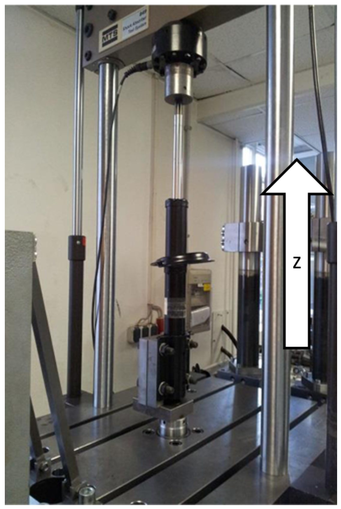
Figure 2.
Modified shock absorber 2
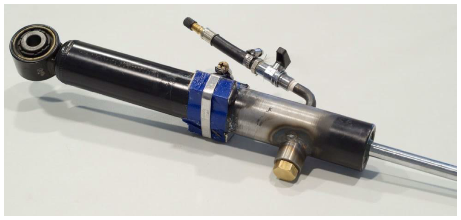
Figure 3.
Force-velocity characteristics of shock absorbers 1 (a) to 8 (h)
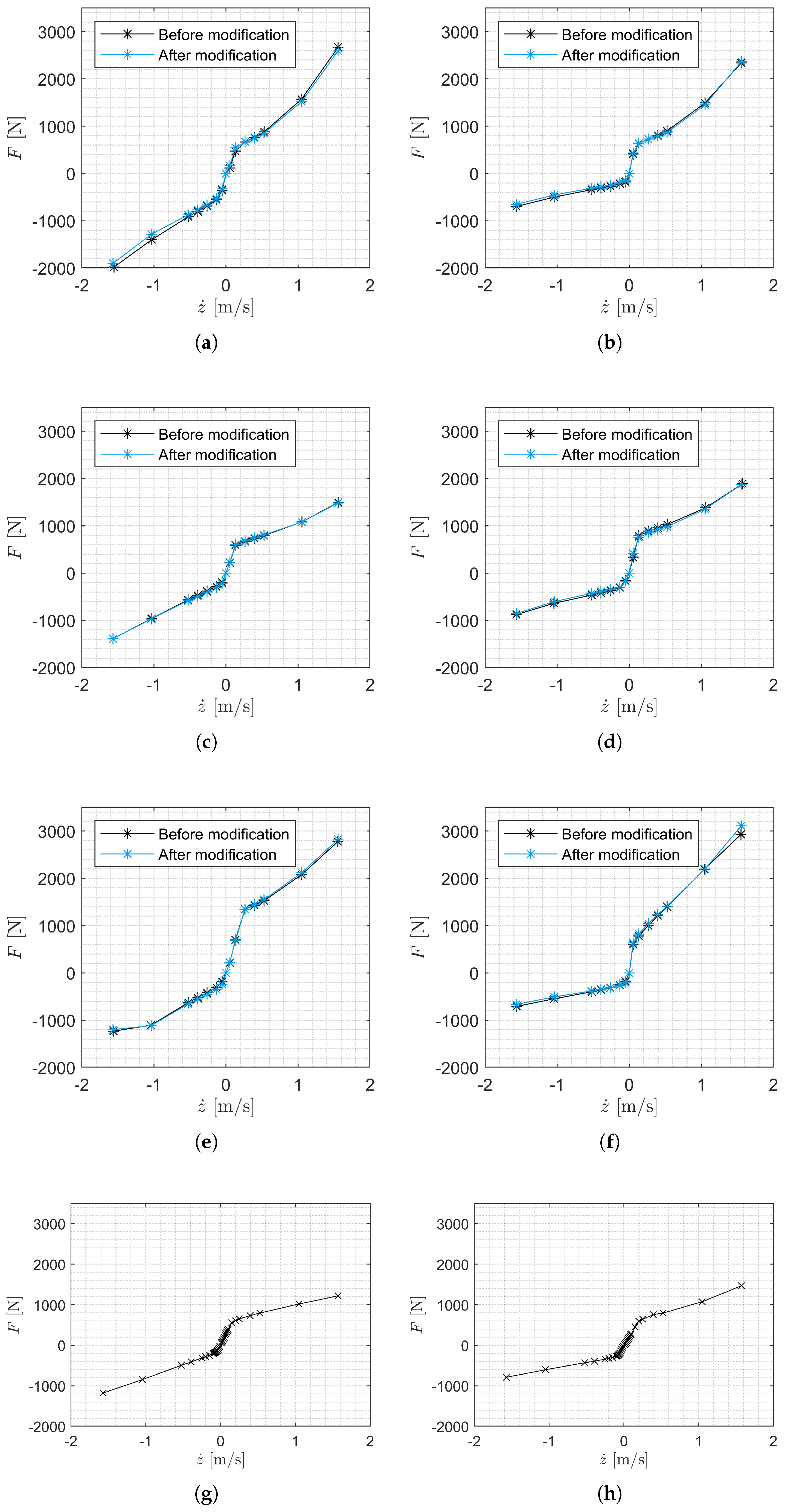
Figure 4.
Front SA excitiations measurements 3 to 7
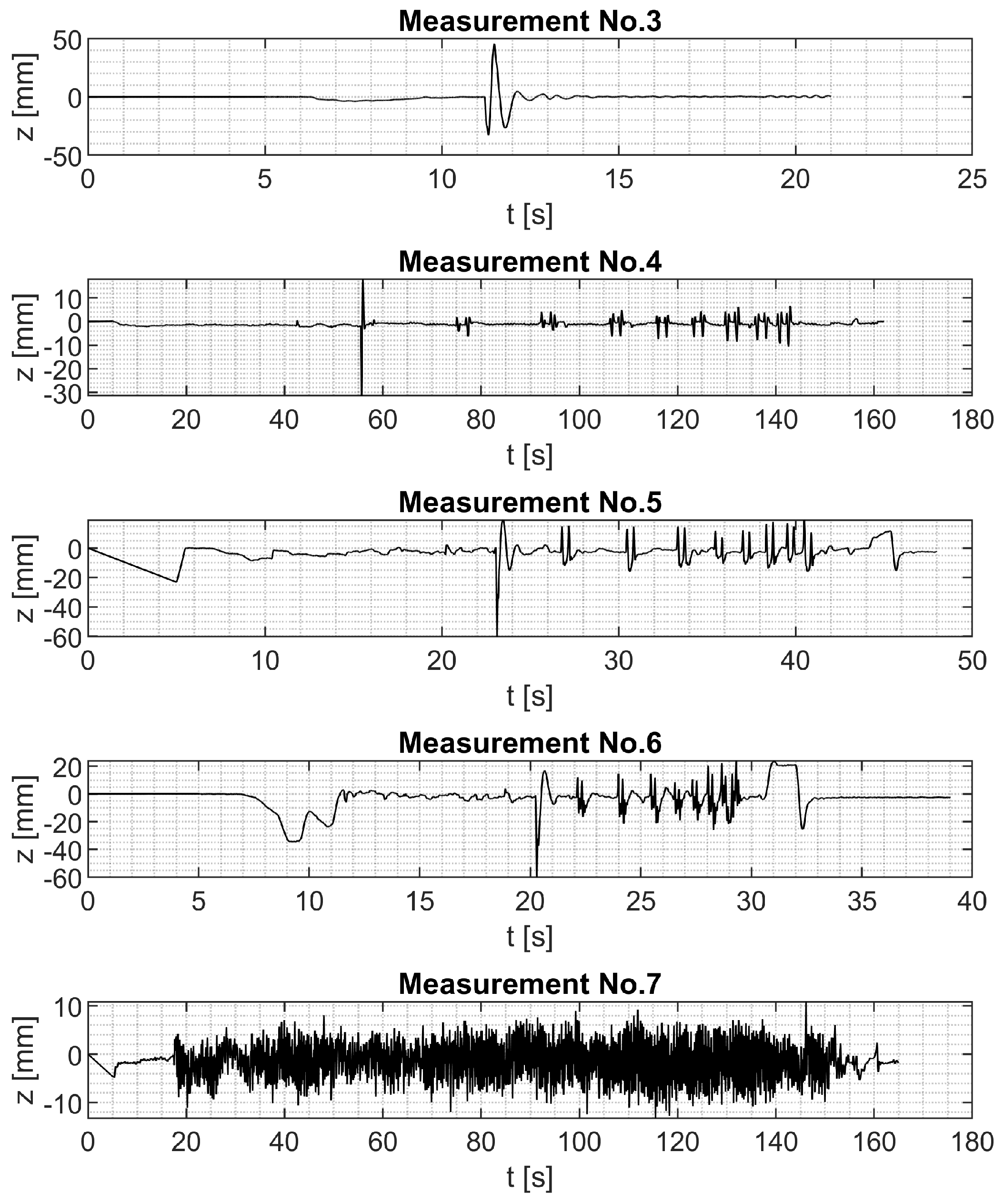
Figure 5.
Front SA excitiations measurements 8 to 12
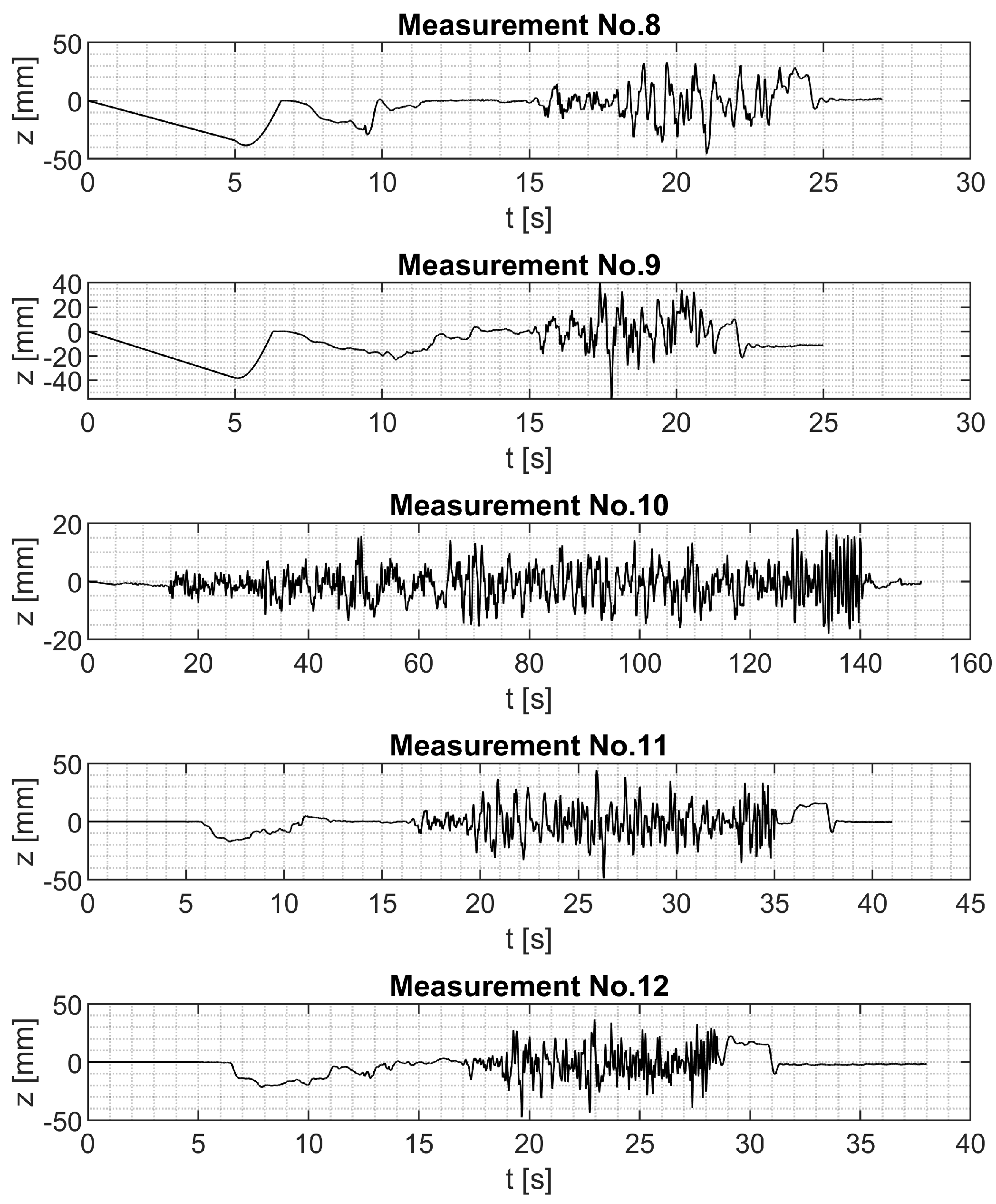
Figure 6.
Shock absorber stroke measurement durcing driving tests
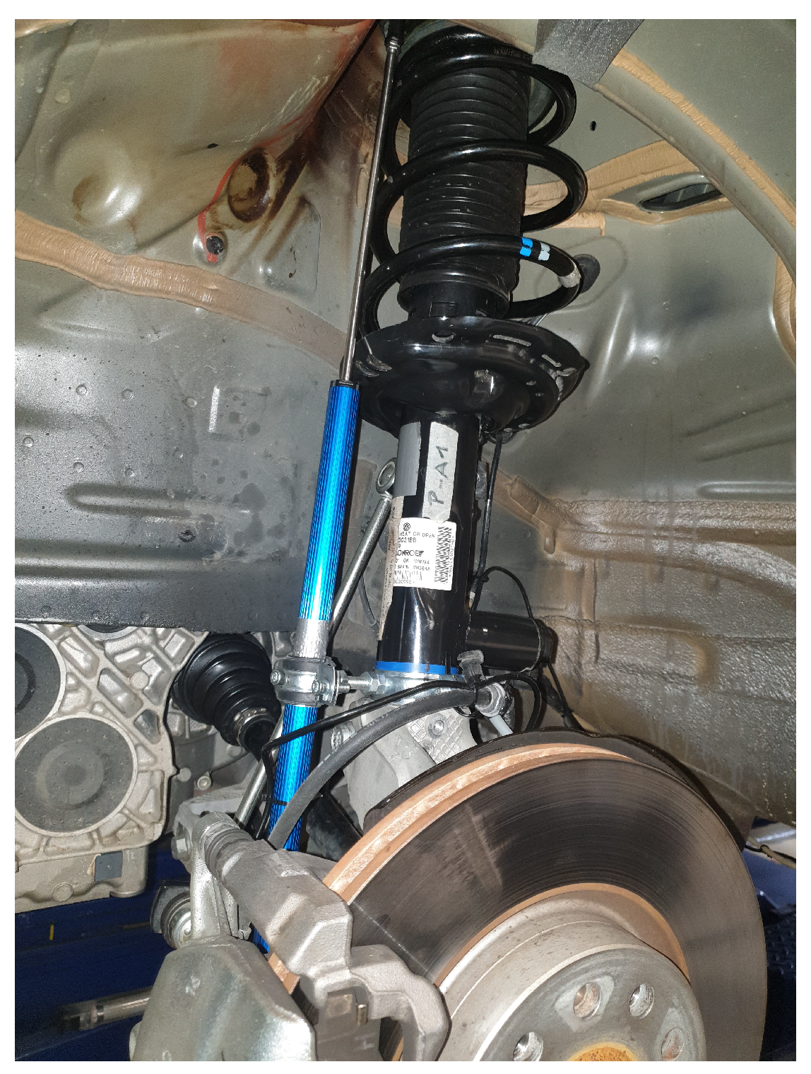
Figure 7.
Quasi-static measurements of shock absorber 7
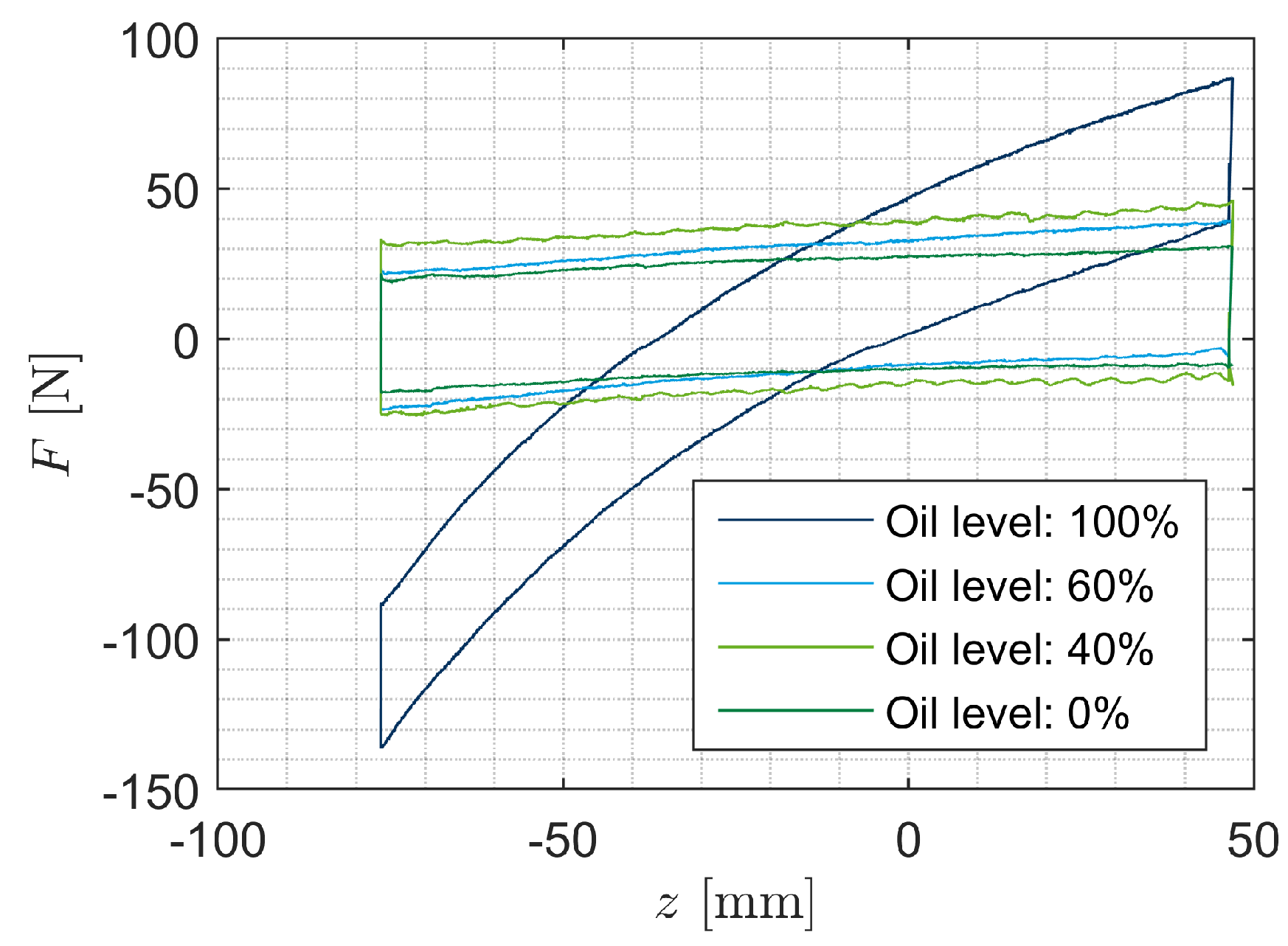
Figure 8.
Force-displacement characteristics of all shock absorbers 1 (a) to (h) for an oil level of 40 % and 100 % of the harmonic measurements with a maximum velocity of 0.05
Figure 8.
Force-displacement characteristics of all shock absorbers 1 (a) to (h) for an oil level of 40 % and 100 % of the harmonic measurements with a maximum velocity of 0.05
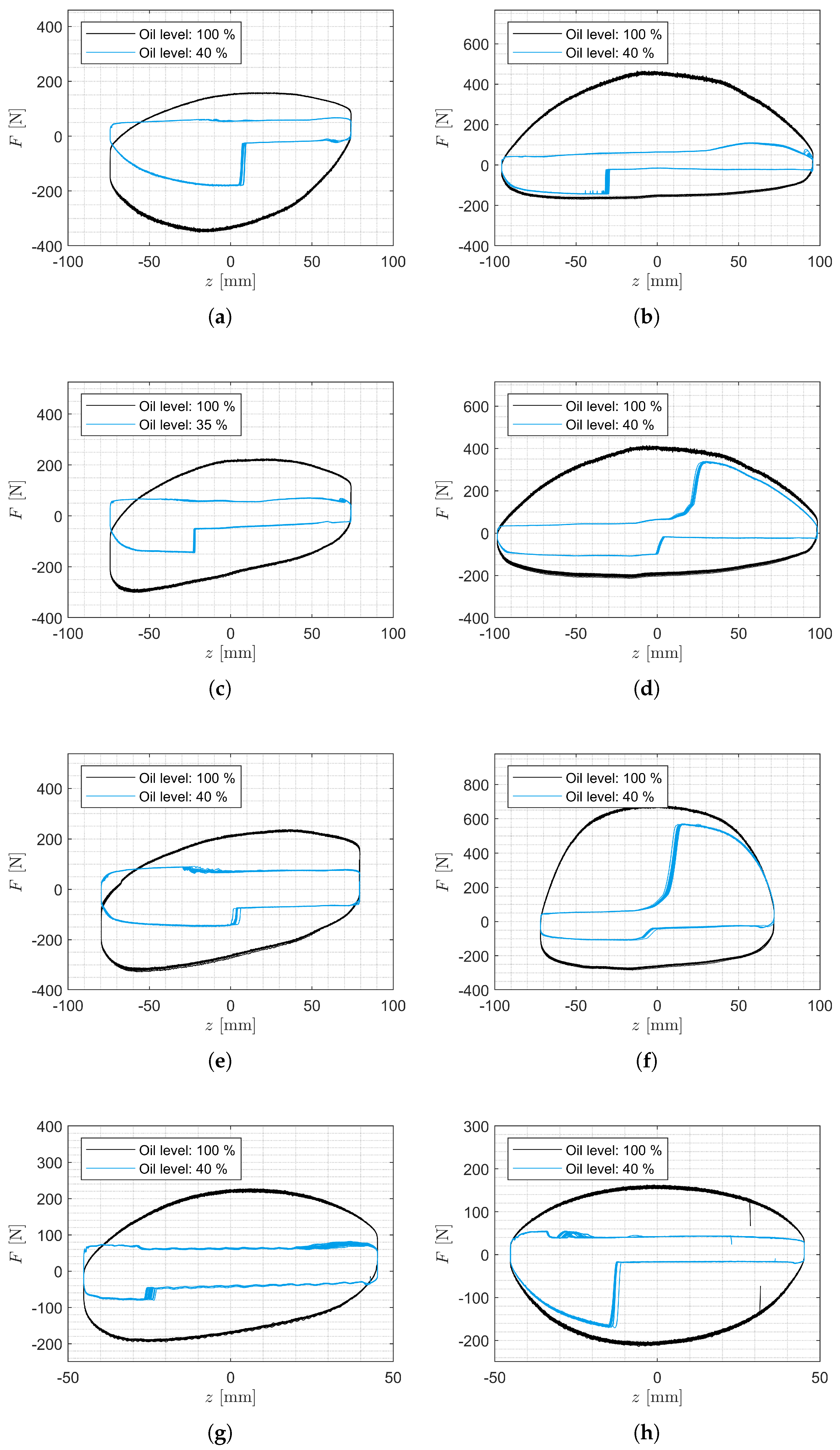
Figure 9.
Force-displacement characteristics of all shock absorbers 1 (a) to 8 (h) for an oil level of 40 % and 100 % respectively for the 19 sinusoidal oscillations with a maximum velocity of 1
Figure 9.
Force-displacement characteristics of all shock absorbers 1 (a) to 8 (h) for an oil level of 40 % and 100 % respectively for the 19 sinusoidal oscillations with a maximum velocity of 1
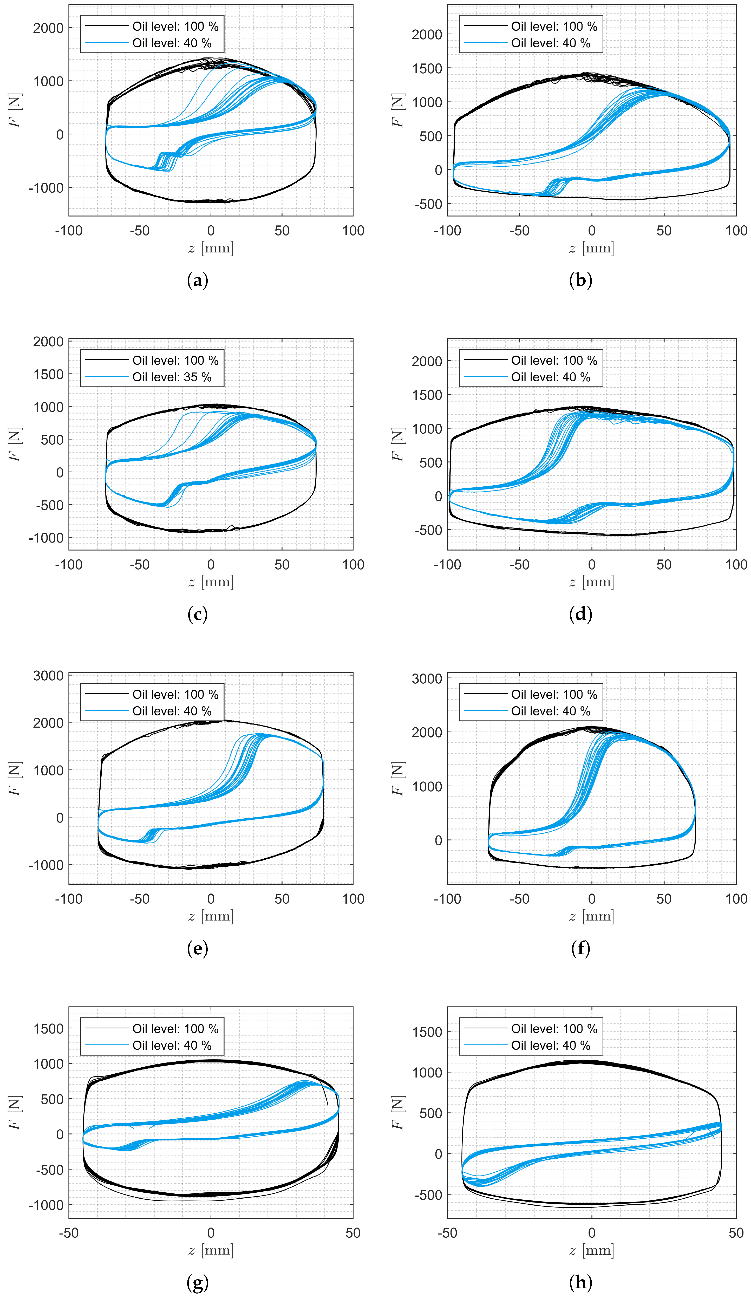
Figure 10.
19 harmonic oscillations with a maximum velocity of 1 m/s for shock absorber 1 with 60 % oil level
Figure 10.
19 harmonic oscillations with a maximum velocity of 1 m/s for shock absorber 1 with 60 % oil level
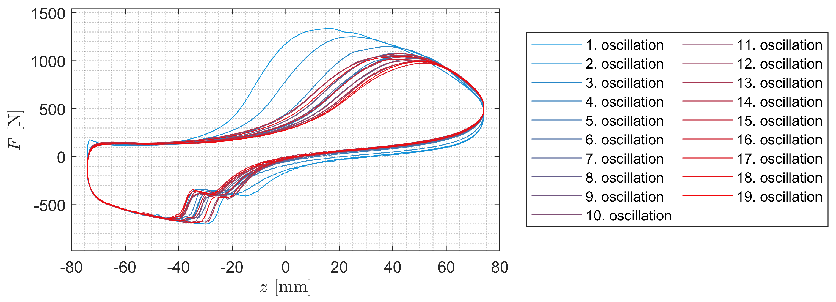
Figure 11.
Work performed by all shock absorbers 1 (a) to 8 (h) with 40 % oil fill level for 19 sinusoidal oscillations
Figure 11.
Work performed by all shock absorbers 1 (a) to 8 (h) with 40 % oil fill level for 19 sinusoidal oscillations
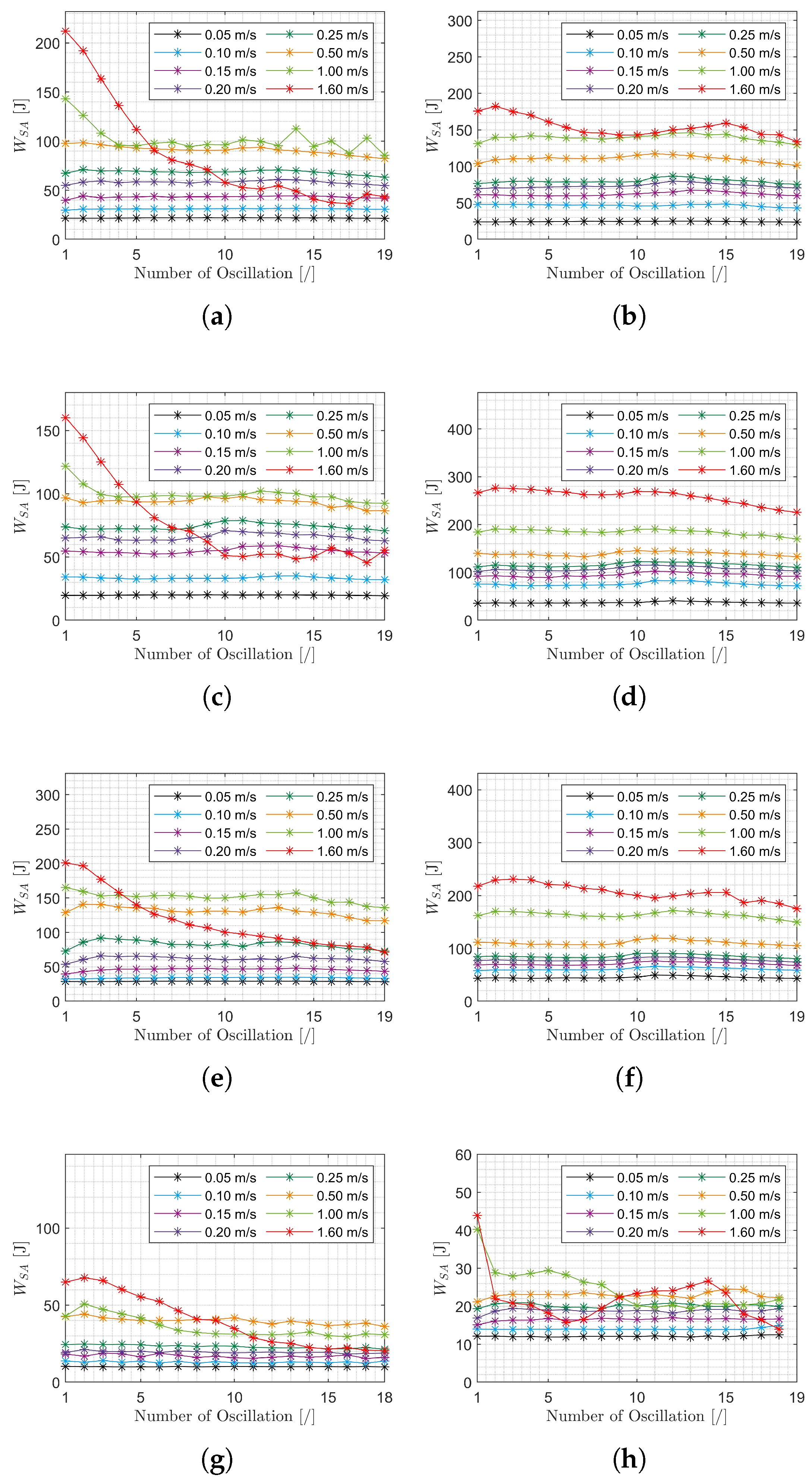
Figure 12.
Velocity dependent scaling factor for the friction force
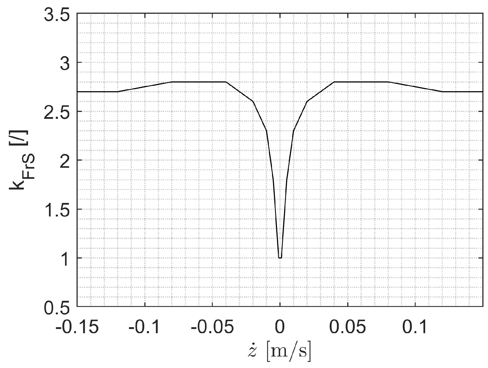
Figure 13.
Twin-tube shock absorber
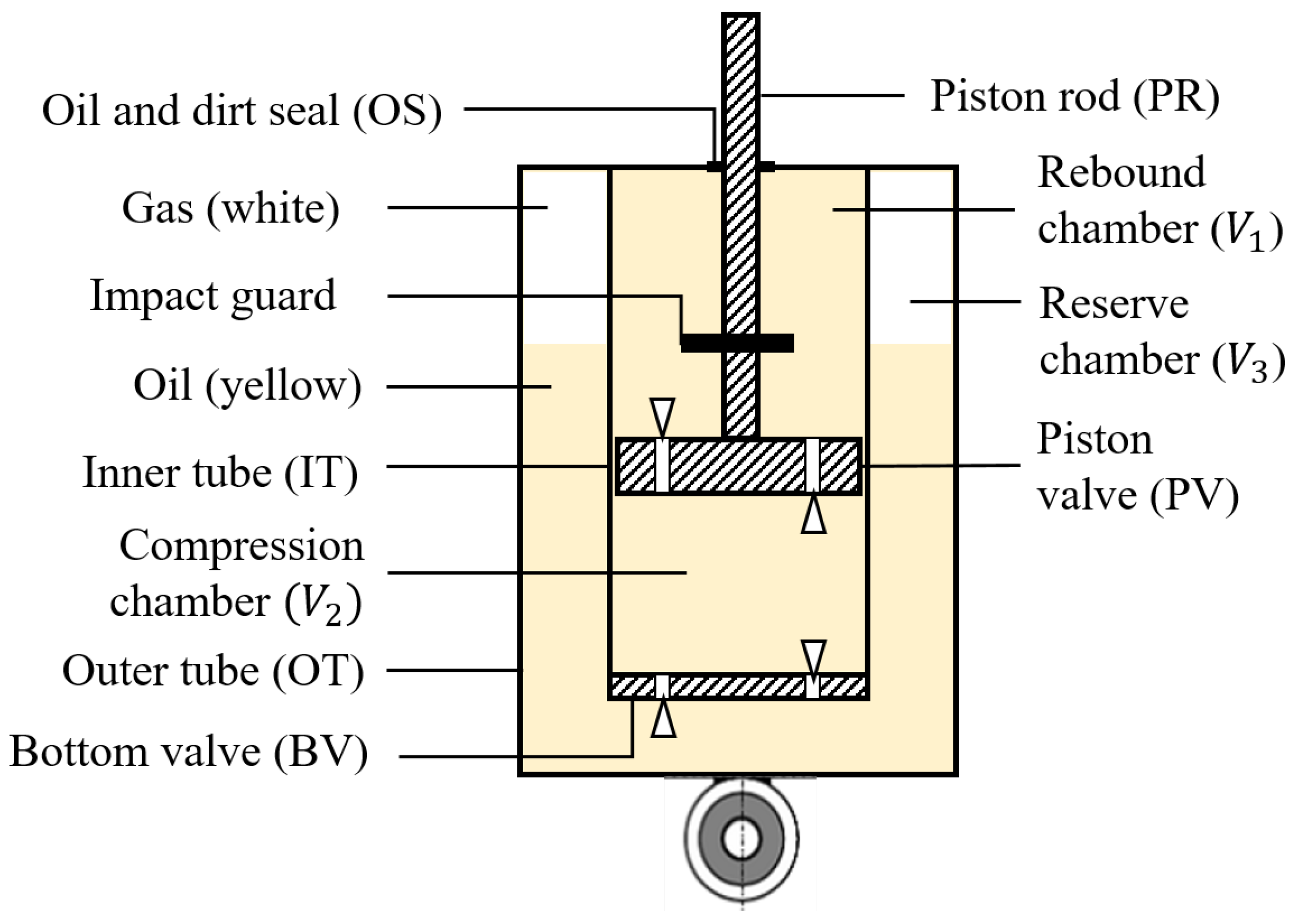
Figure 14.
Volumina of the compression working chamber during harmonic excitation
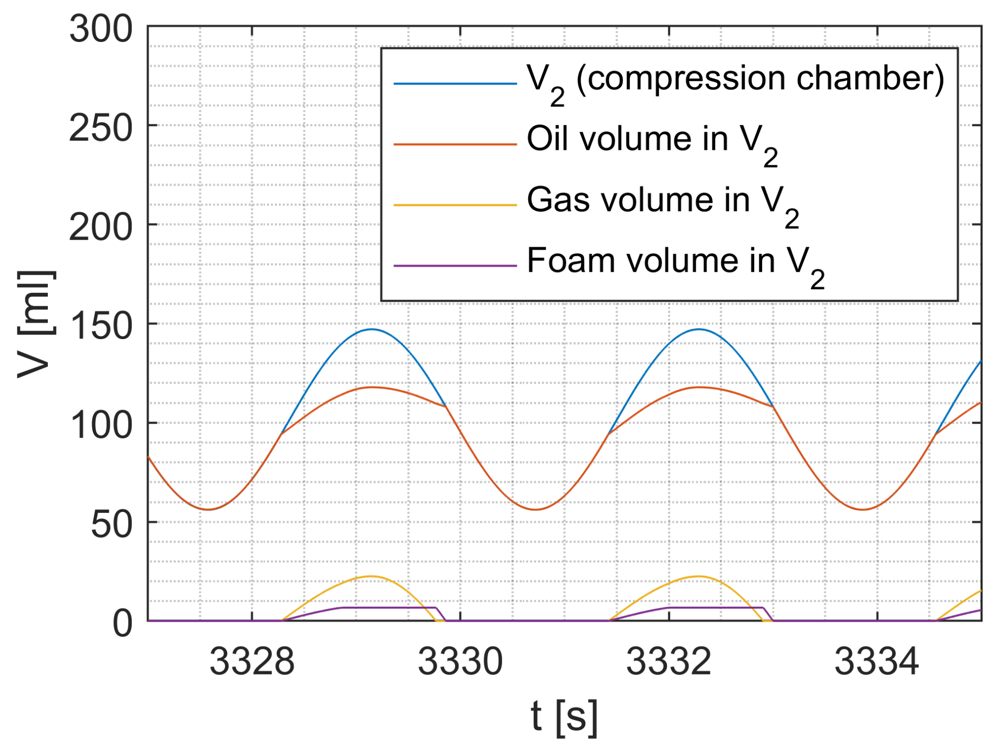
Figure 15.
Shock absorber dimensions
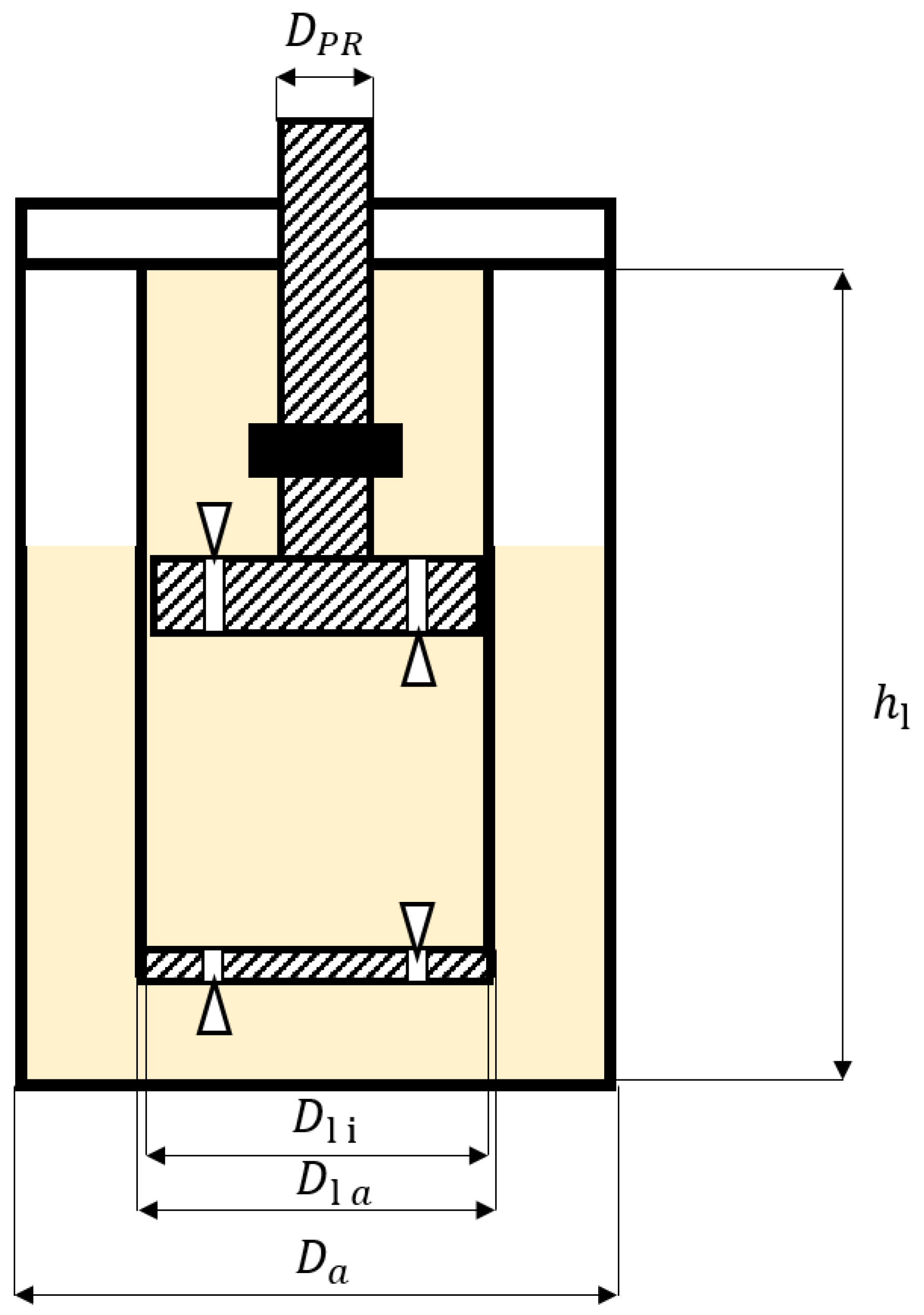
Figure 16.
Effect of model parameters during rebound stroke
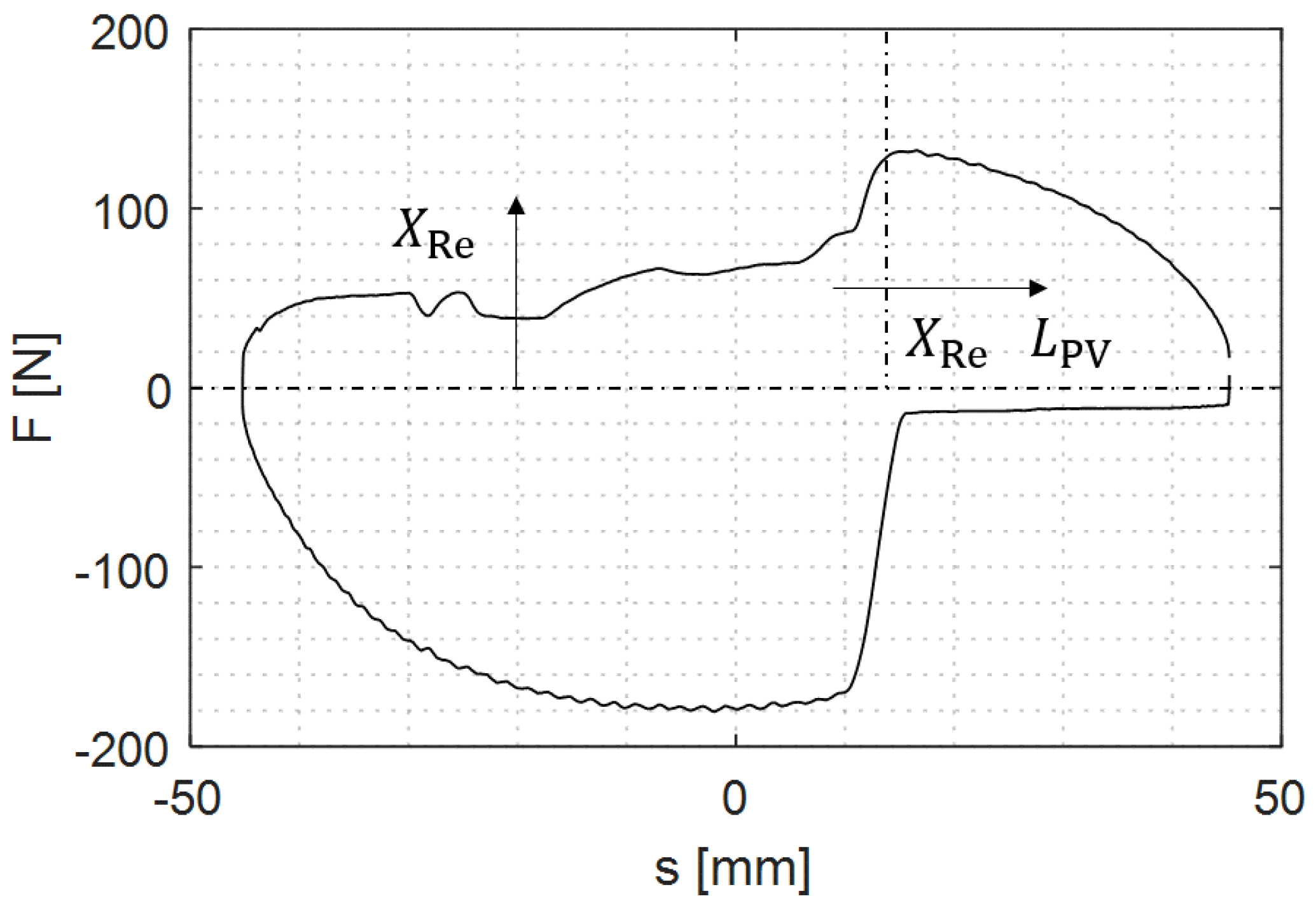
Figure 17.
Effect of model parameters during compression stroke
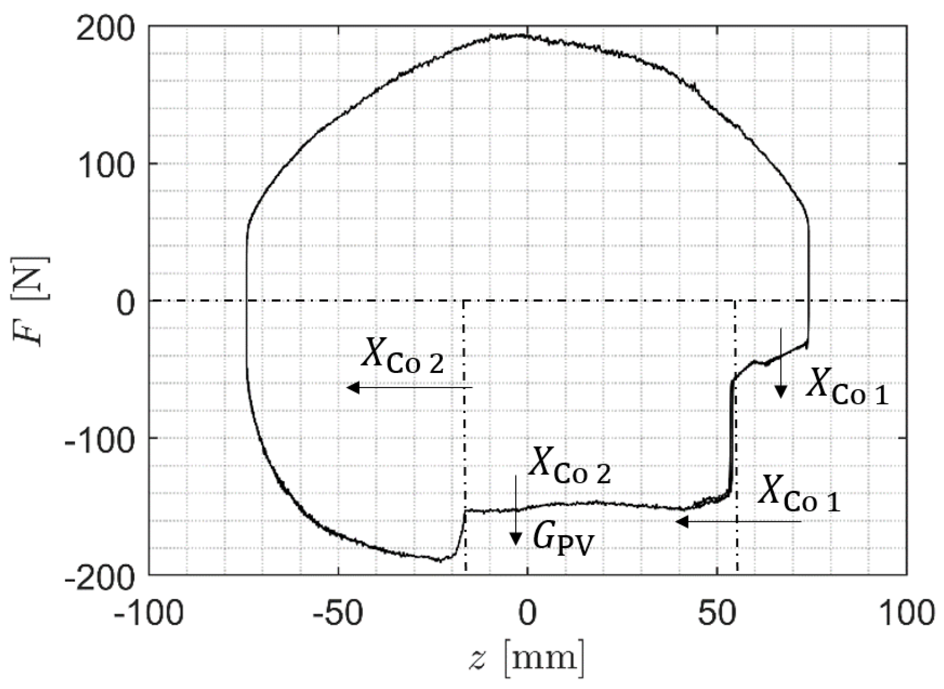
Figure 18.
Depiction of the foaming model (B=1)
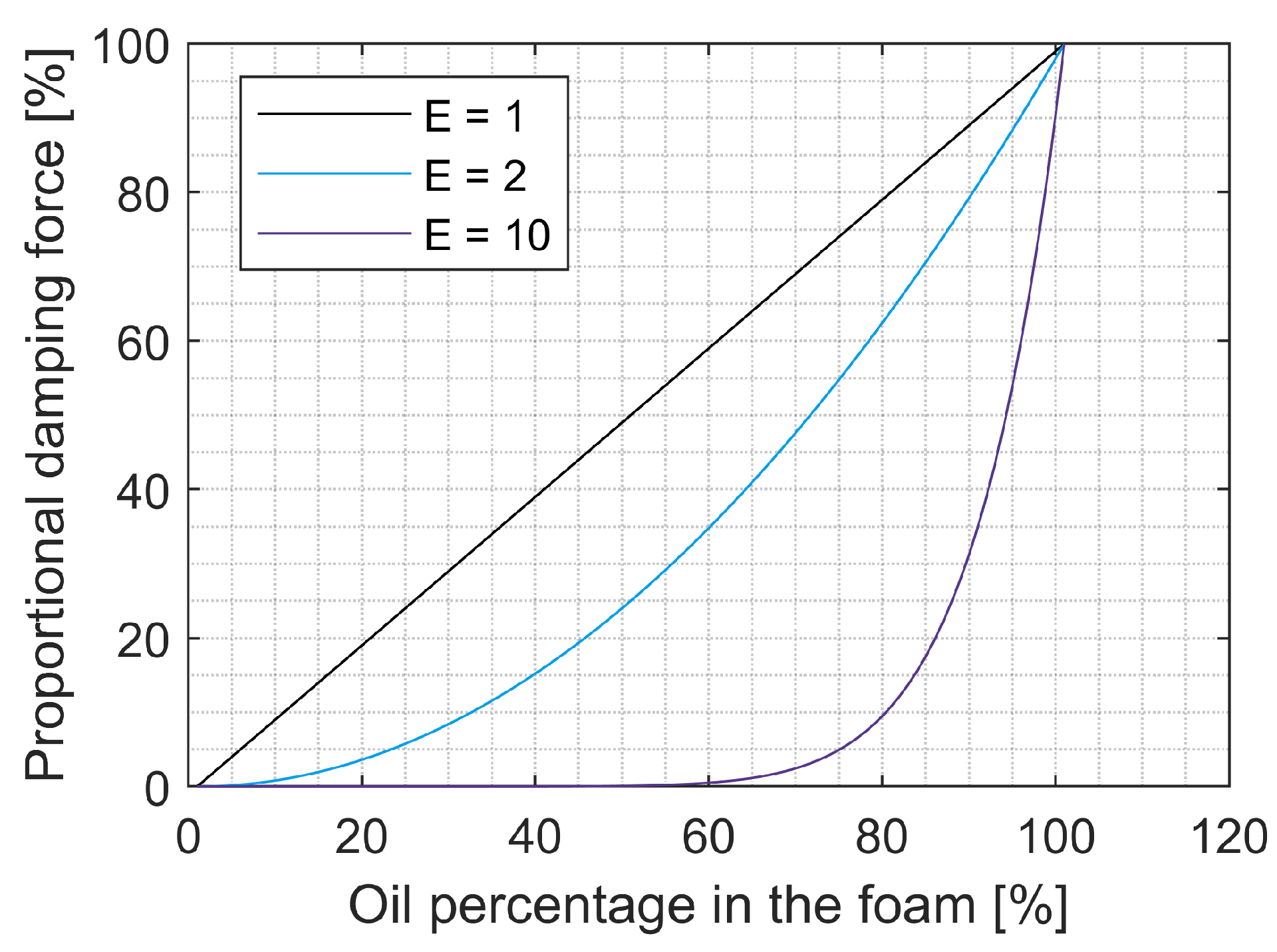
Figure 19.
Damping work for the first oscillation (a) and the 19th oscillation (b) for different excitation velocities of SA 1
Figure 19.
Damping work for the first oscillation (a) and the 19th oscillation (b) for different excitation velocities of SA 1
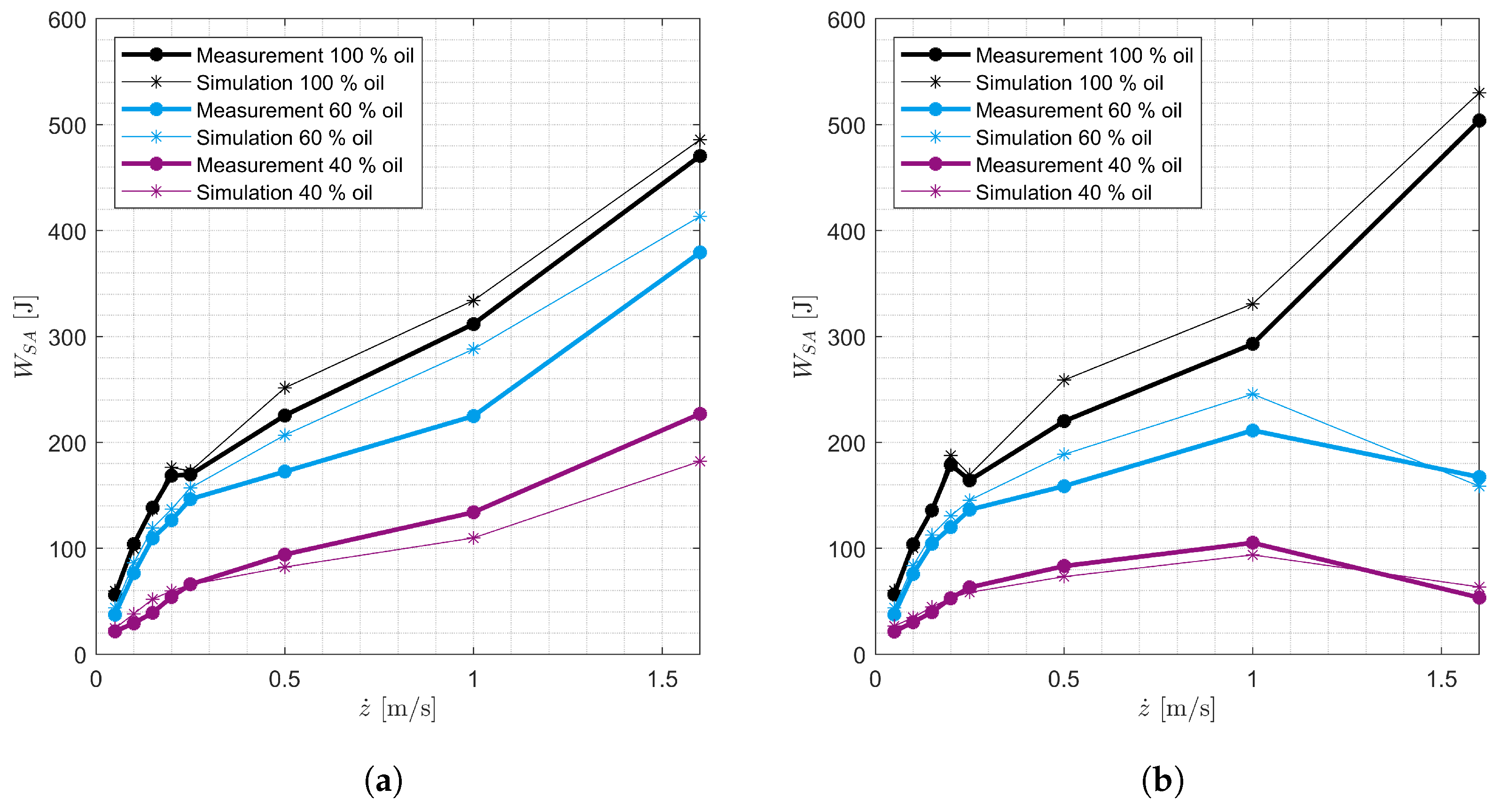
Figure 20.
Damping work for the first oscillation (a) and the 19th oscillation (b) for different excitation velocities of SA 2
Figure 20.
Damping work for the first oscillation (a) and the 19th oscillation (b) for different excitation velocities of SA 2
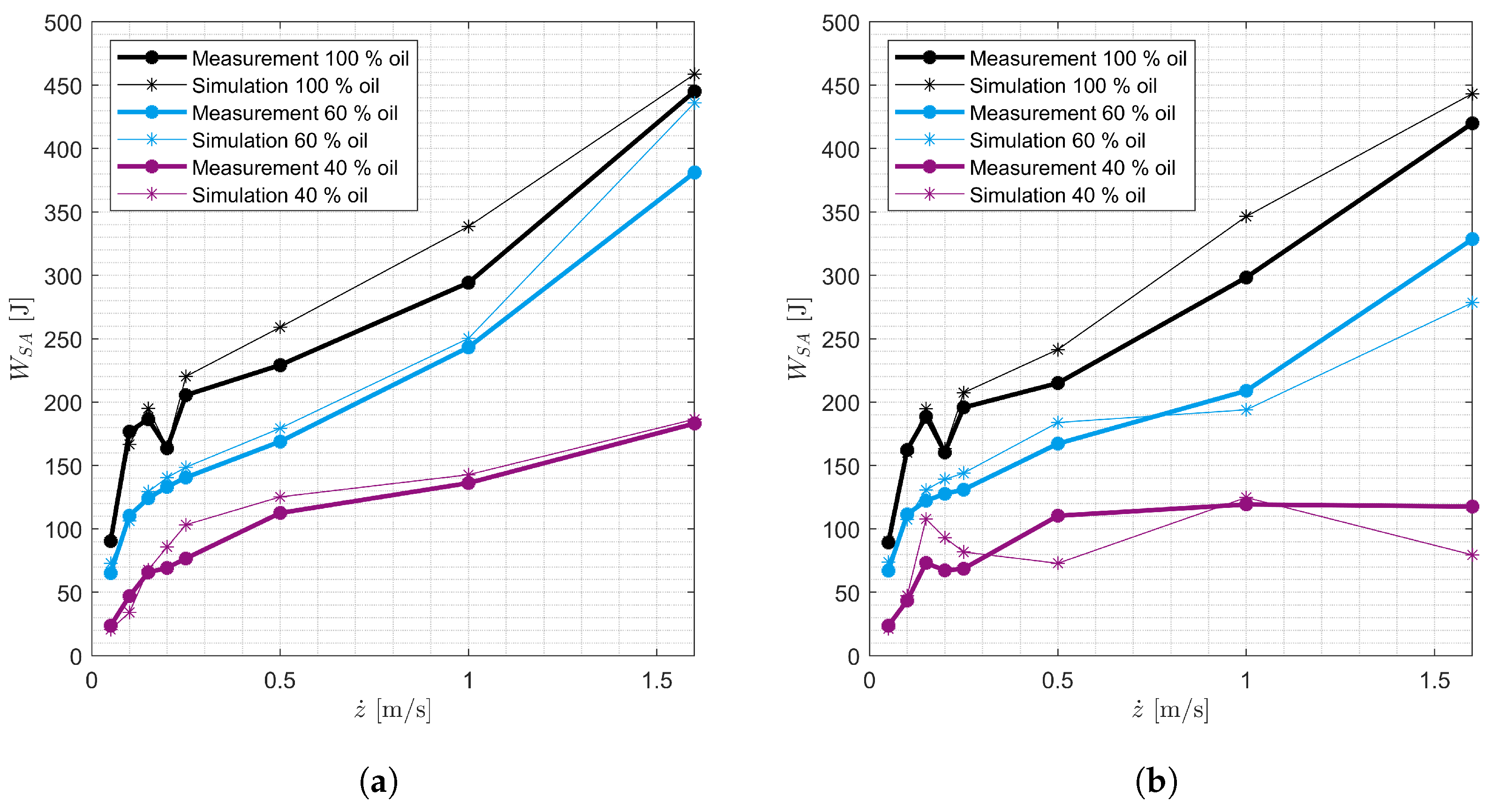
Figure 21.
Damping work for the first oscillation (a) and the 19th oscillation (b) for different excitation velocities of SA 3
Figure 21.
Damping work for the first oscillation (a) and the 19th oscillation (b) for different excitation velocities of SA 3
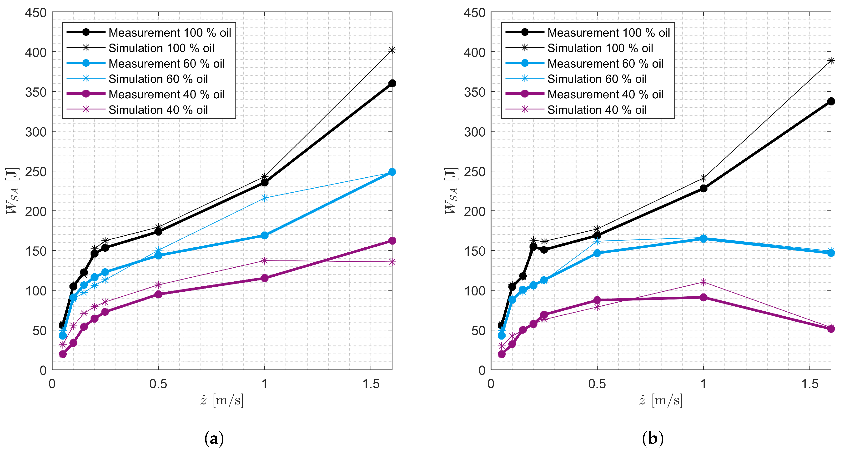
Figure 22.
Damping work for the first oscillation (a) and the 19th oscillation (b) for different excitation velocities of SA 4
Figure 22.
Damping work for the first oscillation (a) and the 19th oscillation (b) for different excitation velocities of SA 4
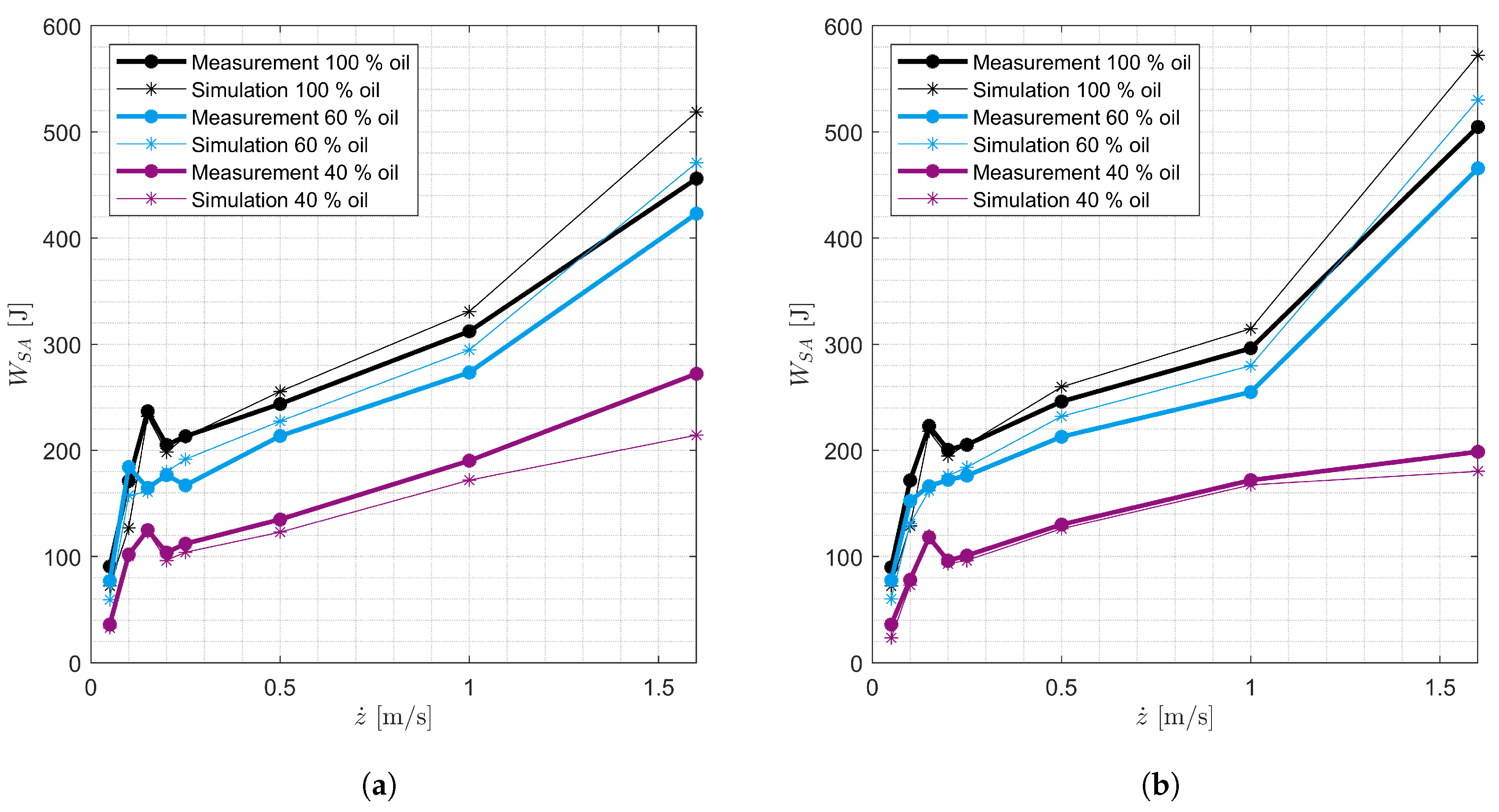
Figure 23.
Damping work for the first oscillation (a) and the 19th oscillation (b) for different excitation velocities of SA 5
Figure 23.
Damping work for the first oscillation (a) and the 19th oscillation (b) for different excitation velocities of SA 5
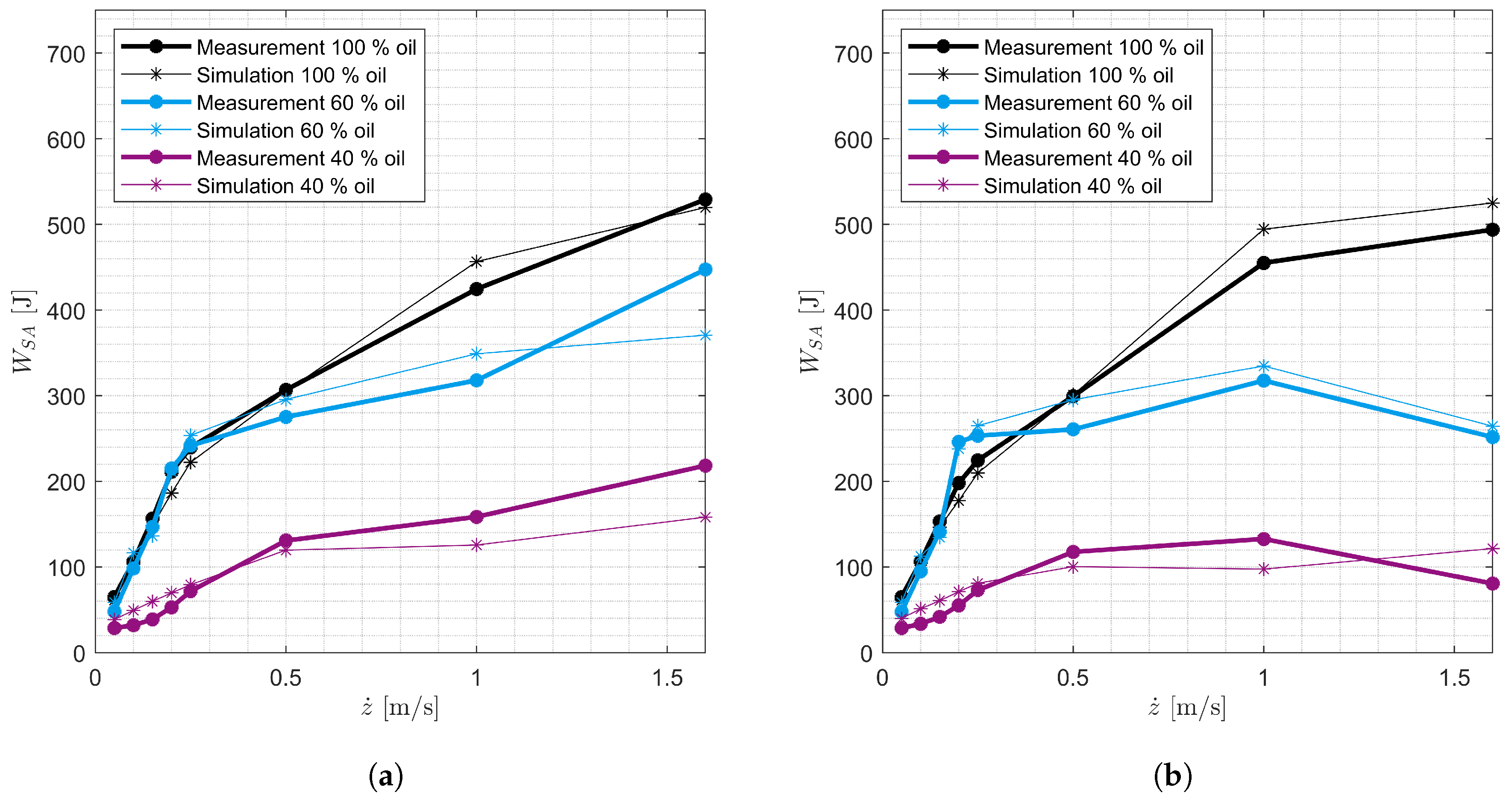
Figure 24.
Damping work for the first oscillation (a) and the 19th oscillation (b) for different excitation velocities of SA 6
Figure 24.
Damping work for the first oscillation (a) and the 19th oscillation (b) for different excitation velocities of SA 6
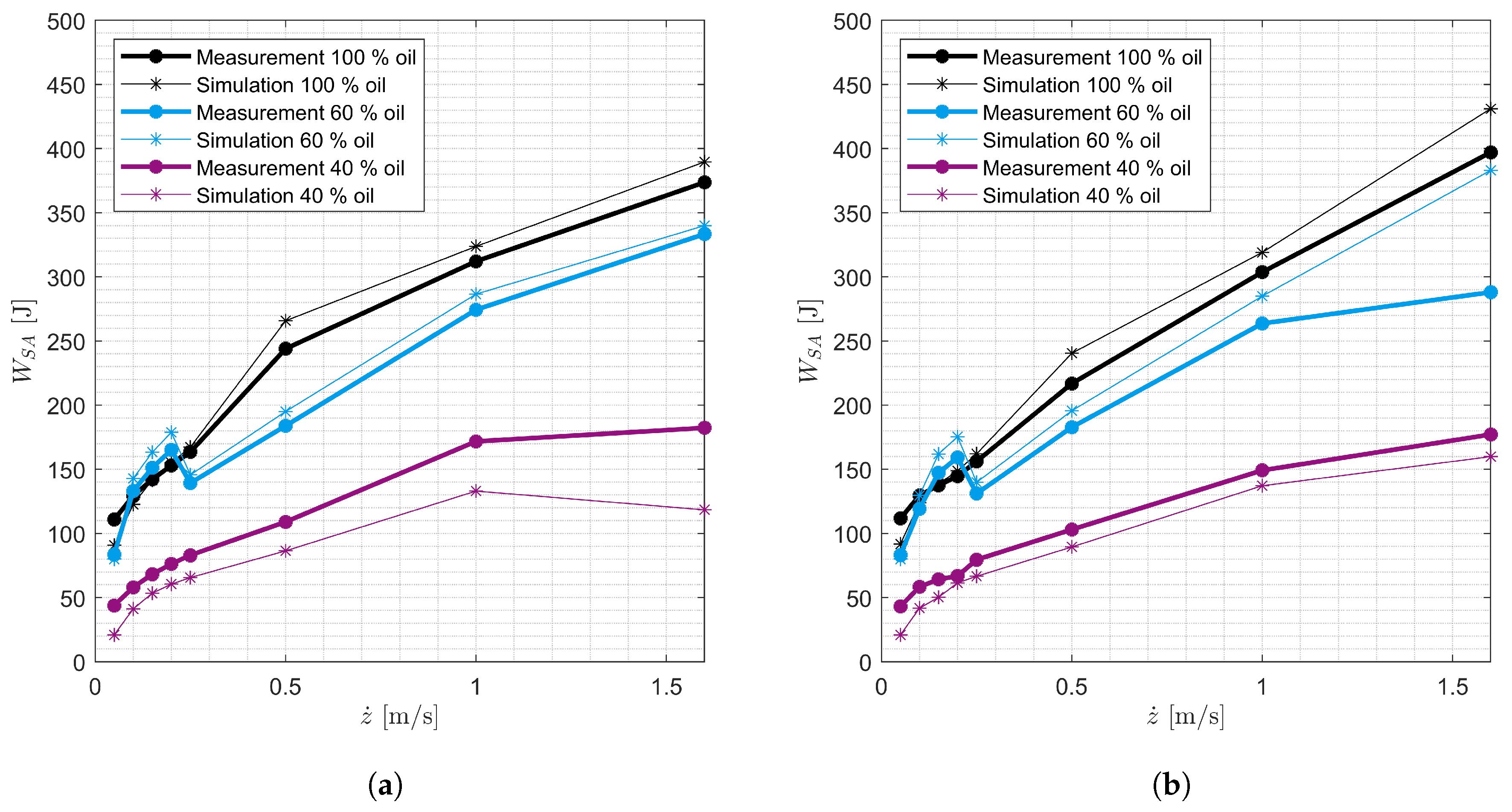
Figure 25.
Damping work for the first oscillation (a) and the 19th oscillation (b) for different excitation velocities of SA 7
Figure 25.
Damping work for the first oscillation (a) and the 19th oscillation (b) for different excitation velocities of SA 7
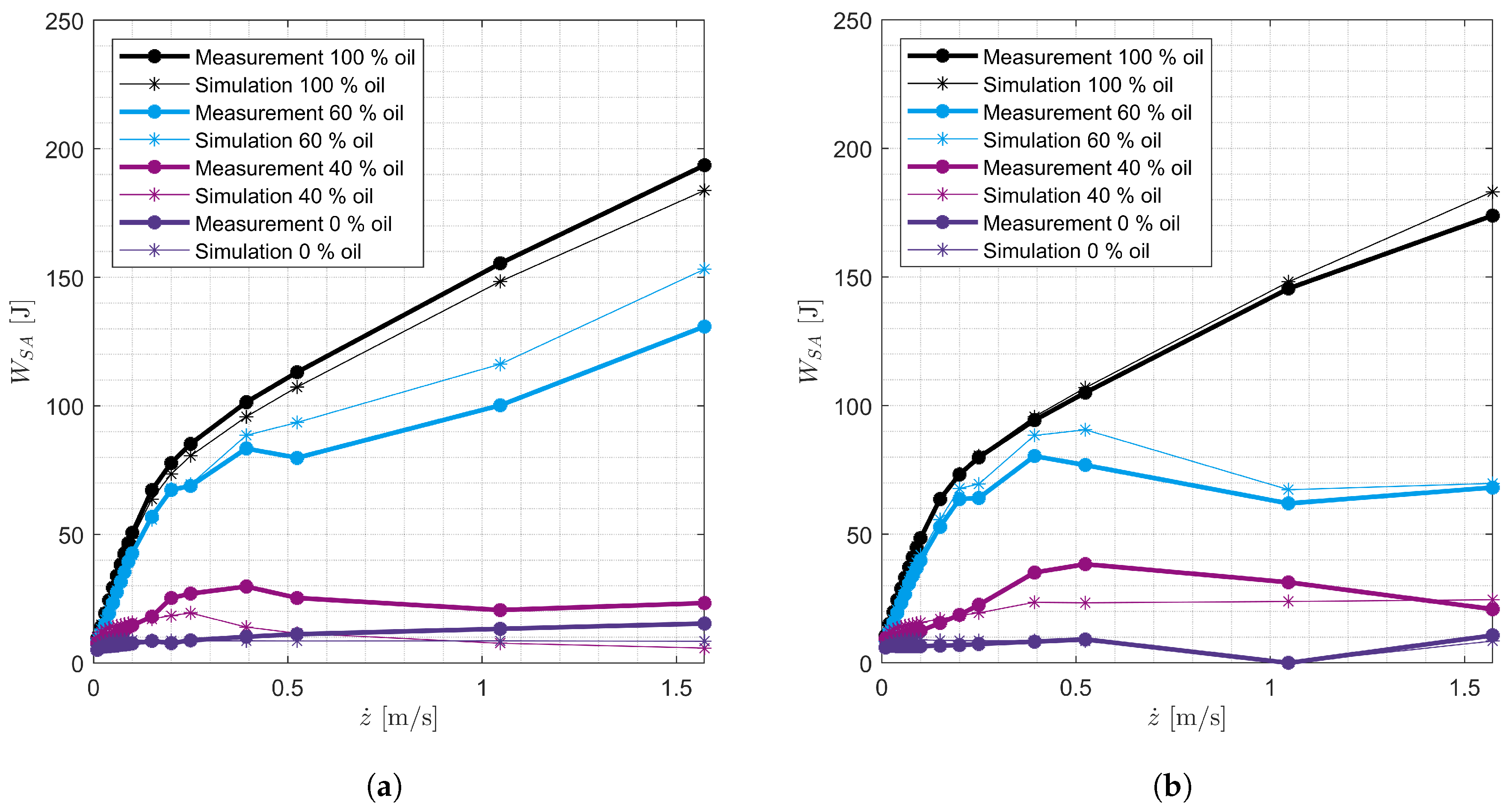
Figure 26.
Damping work for the first oscillation (a) and the 19th oscillation (b) for different excitation velocities of SA 8
Figure 26.
Damping work for the first oscillation (a) and the 19th oscillation (b) for different excitation velocities of SA 8
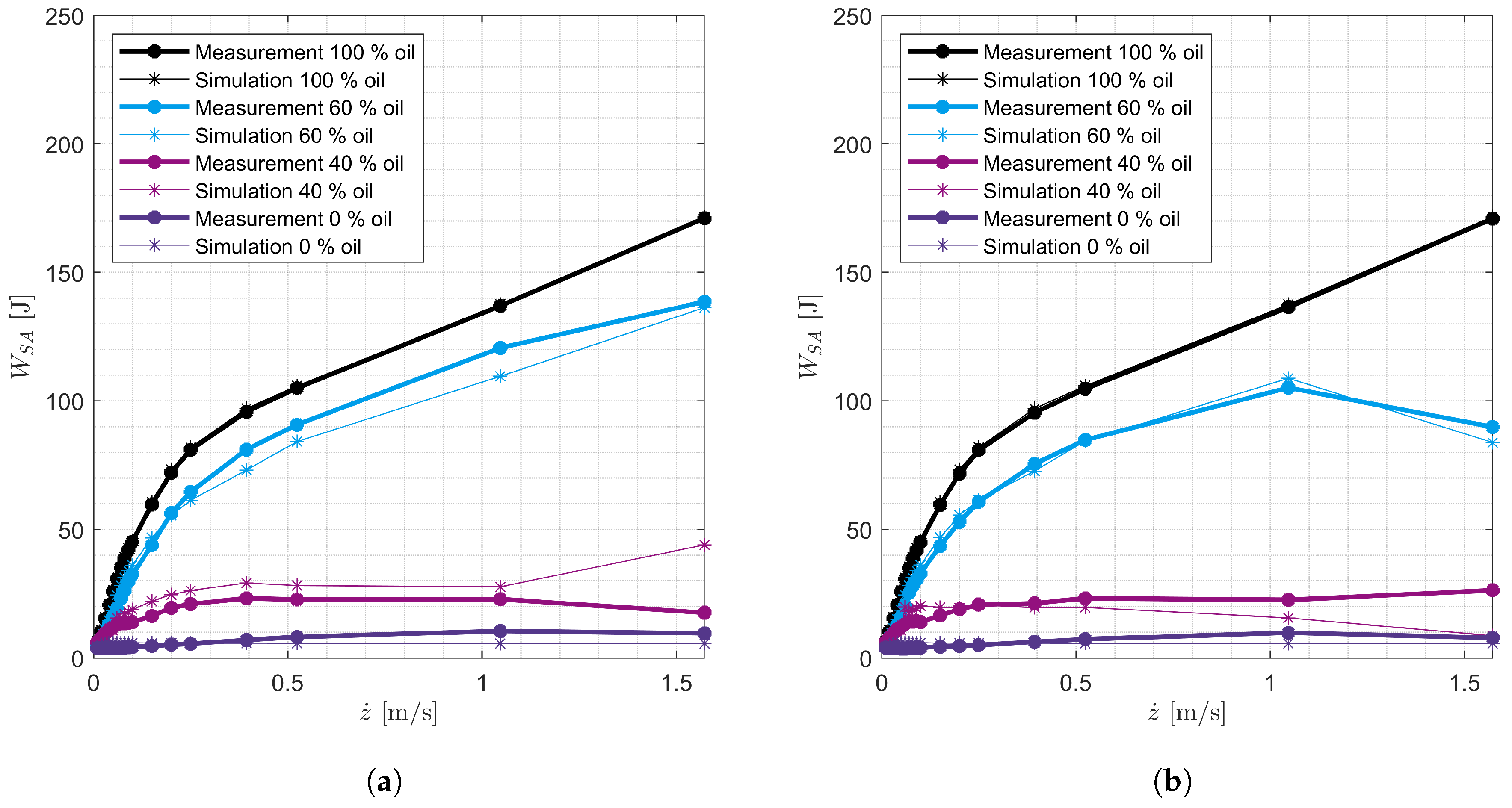
Figure 27.
Force-displacement diagram of SA 7 with 60 % oil level for a harmonic oscillation with a maximum velocity of 0.08 m/s
Figure 27.
Force-displacement diagram of SA 7 with 60 % oil level for a harmonic oscillation with a maximum velocity of 0.08 m/s
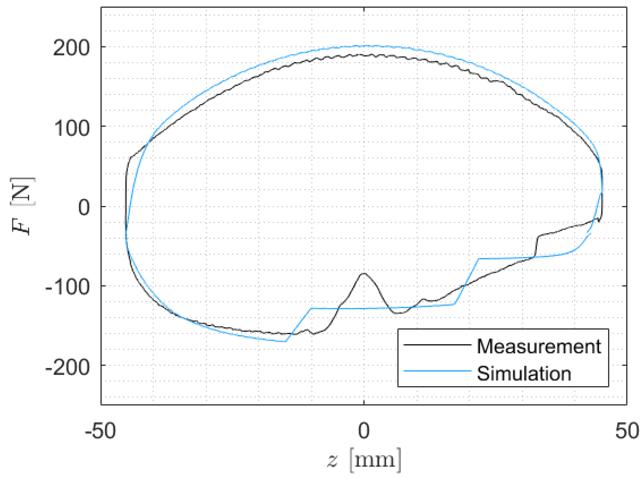
Figure 28.
Force-displacement diagram of SA 7 with 60 % oil level for 19 harmonic oscillations with a maximum velocity of 1.572 m/s
Figure 28.
Force-displacement diagram of SA 7 with 60 % oil level for 19 harmonic oscillations with a maximum velocity of 1.572 m/s
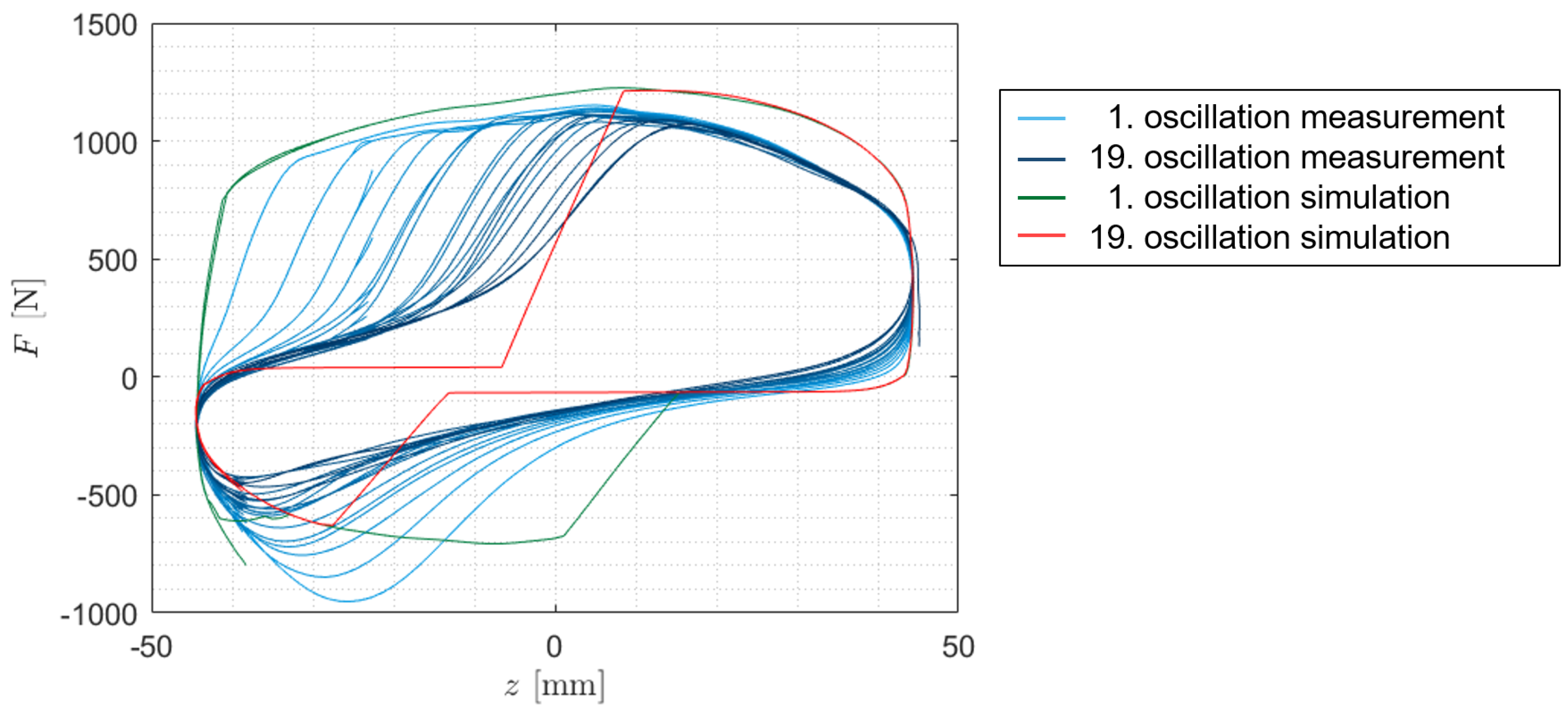
Figure 29.
Damping force over time for the slow bump crossing of SA 7
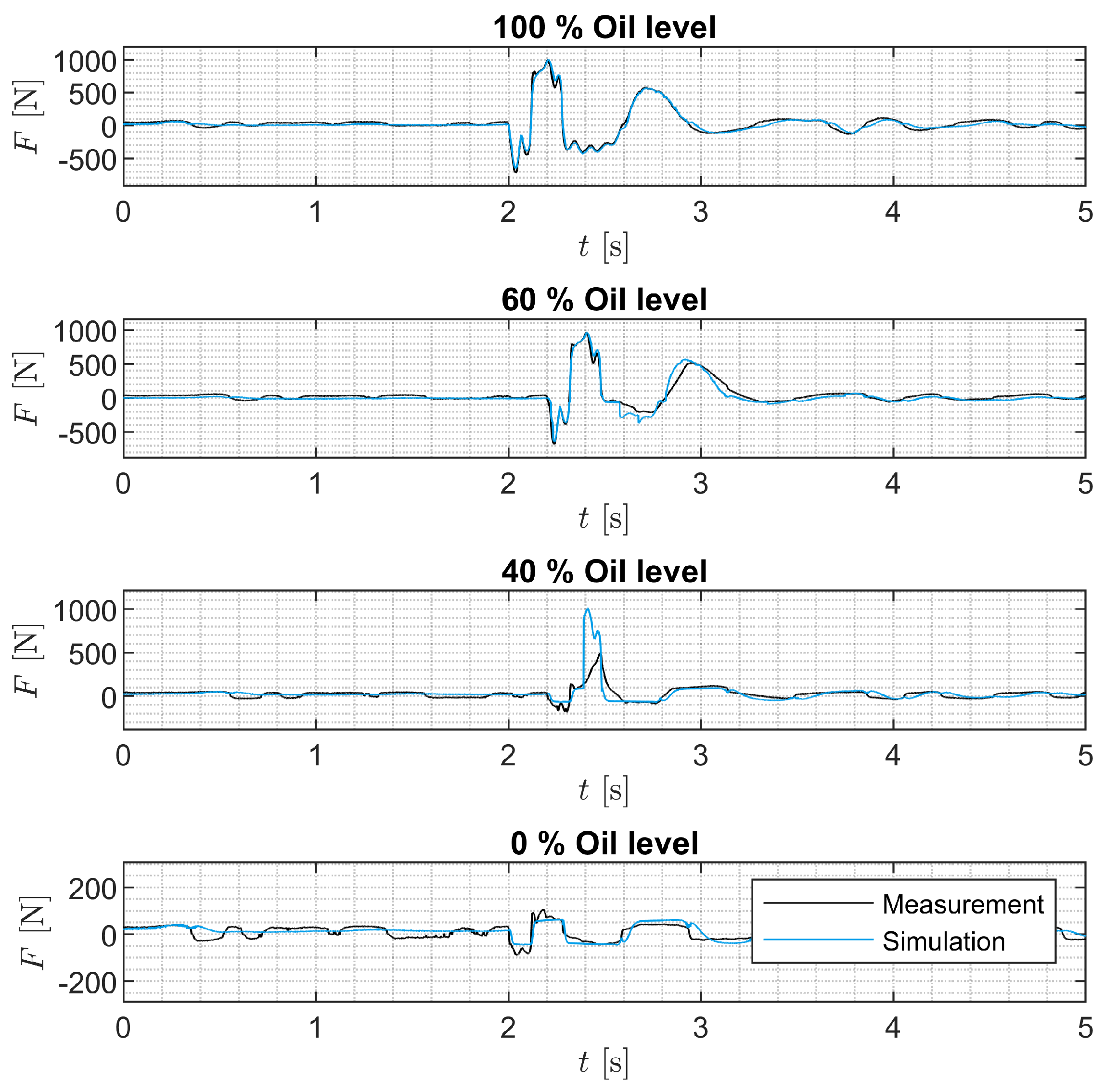
Figure 30.
Damping force over time for the slow bump crossing of SA 8
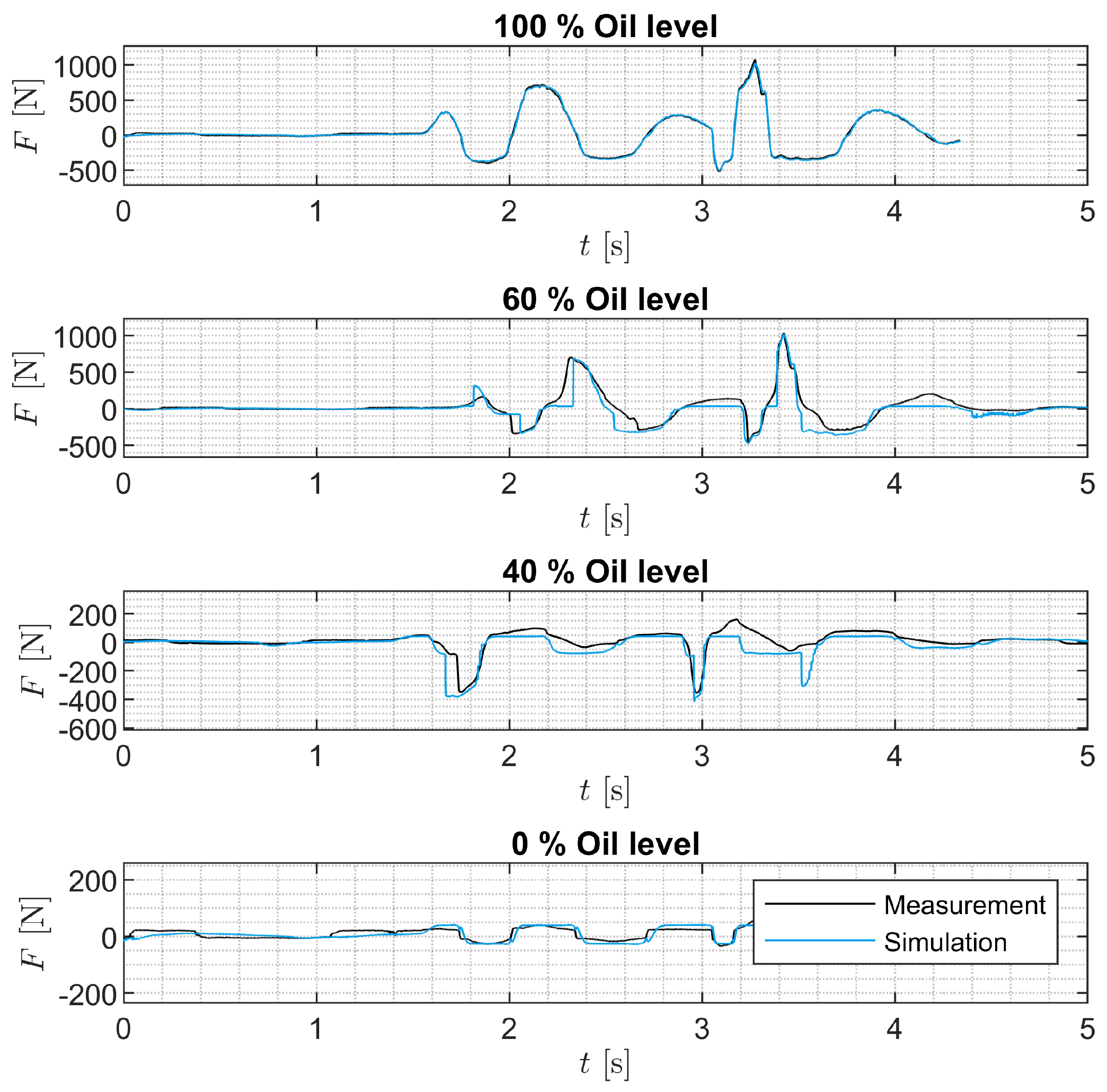
Figure 31.
Work performed for stochastic excitation signals of SA 7
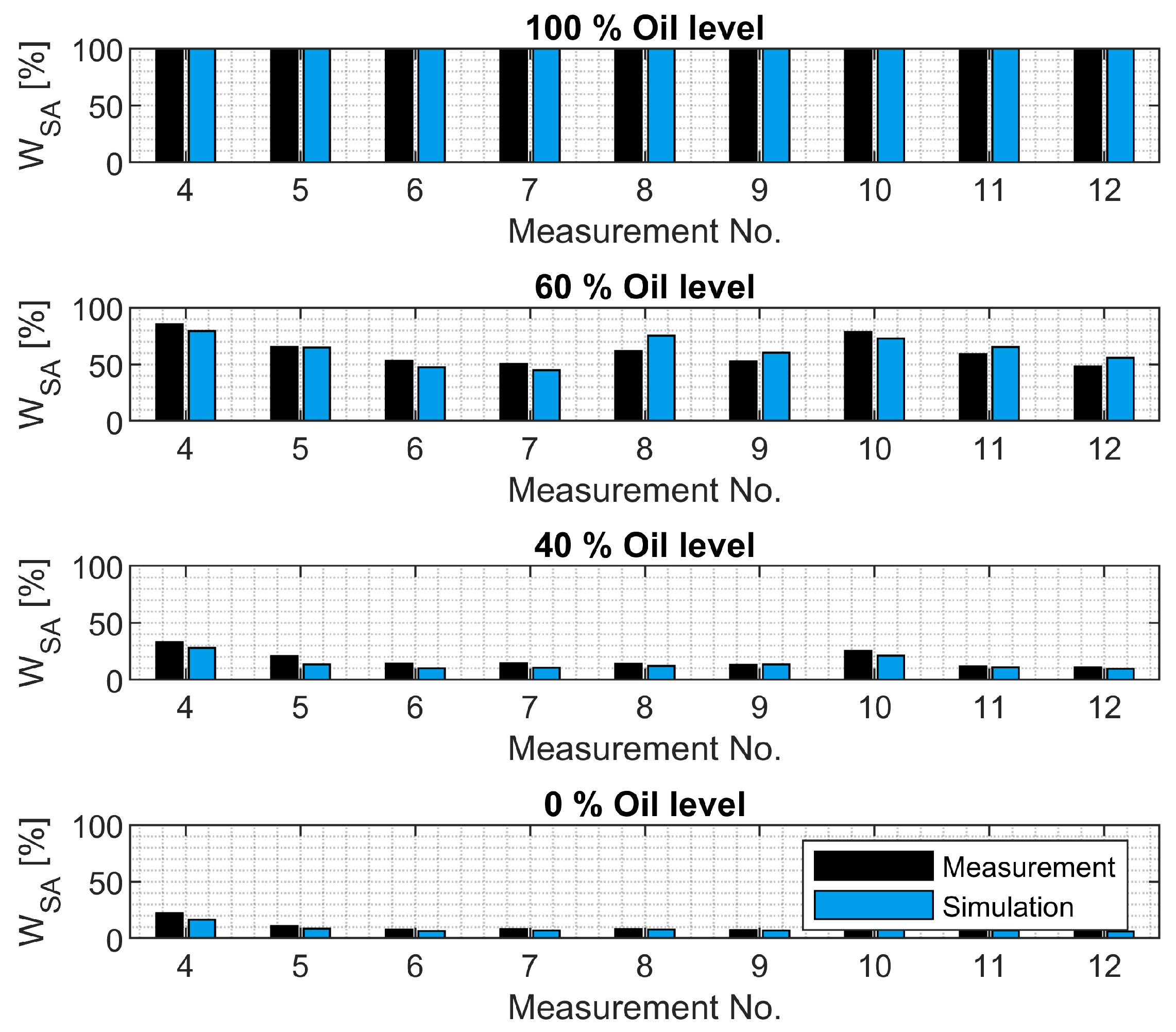
Figure 32.
Work performed for stochastic excitation signals of SA 8
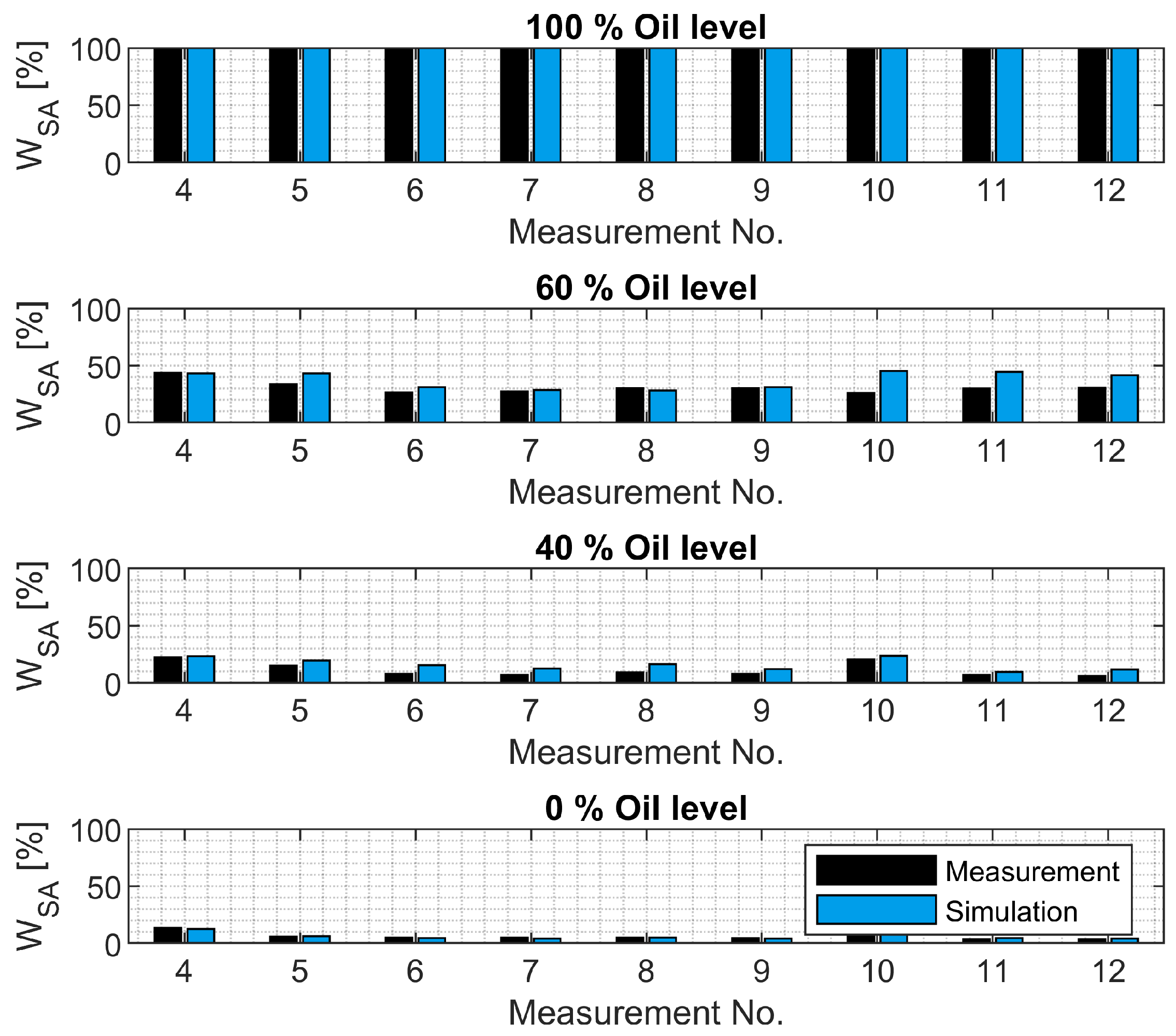
Figure 33.
Damping work for the 1st oscillation (a) and the 19th oscillation (b) for different velocities and model variants for SA 8
Figure 33.
Damping work for the 1st oscillation (a) and the 19th oscillation (b) for different velocities and model variants for SA 8
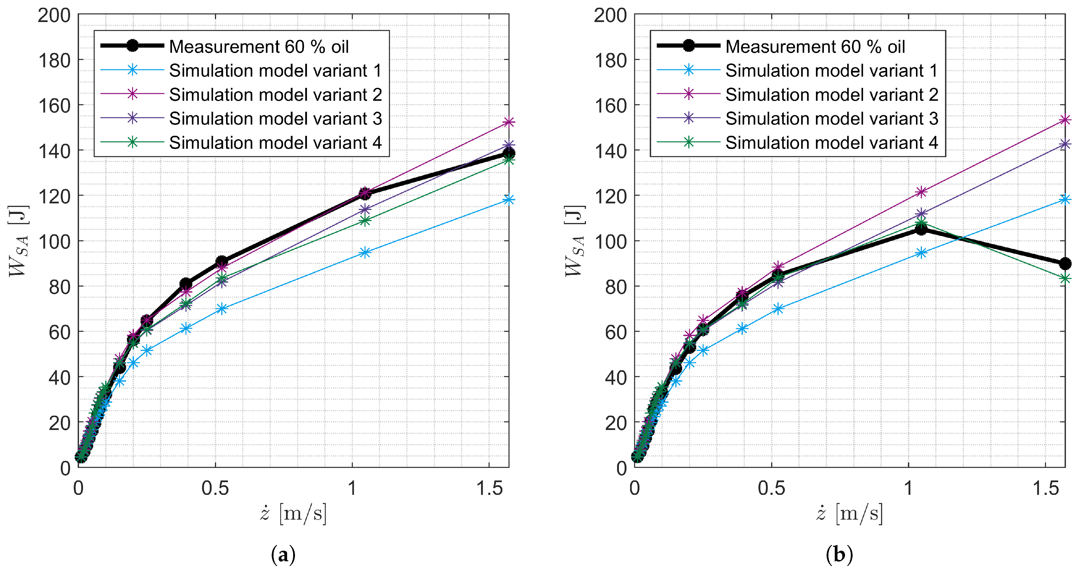
Figure 34.
Damping work for the 1st oscillation and the 19th oscillation for different velocities and different oil levels for SA 8
Figure 34.
Damping work for the 1st oscillation and the 19th oscillation for different velocities and different oil levels for SA 8
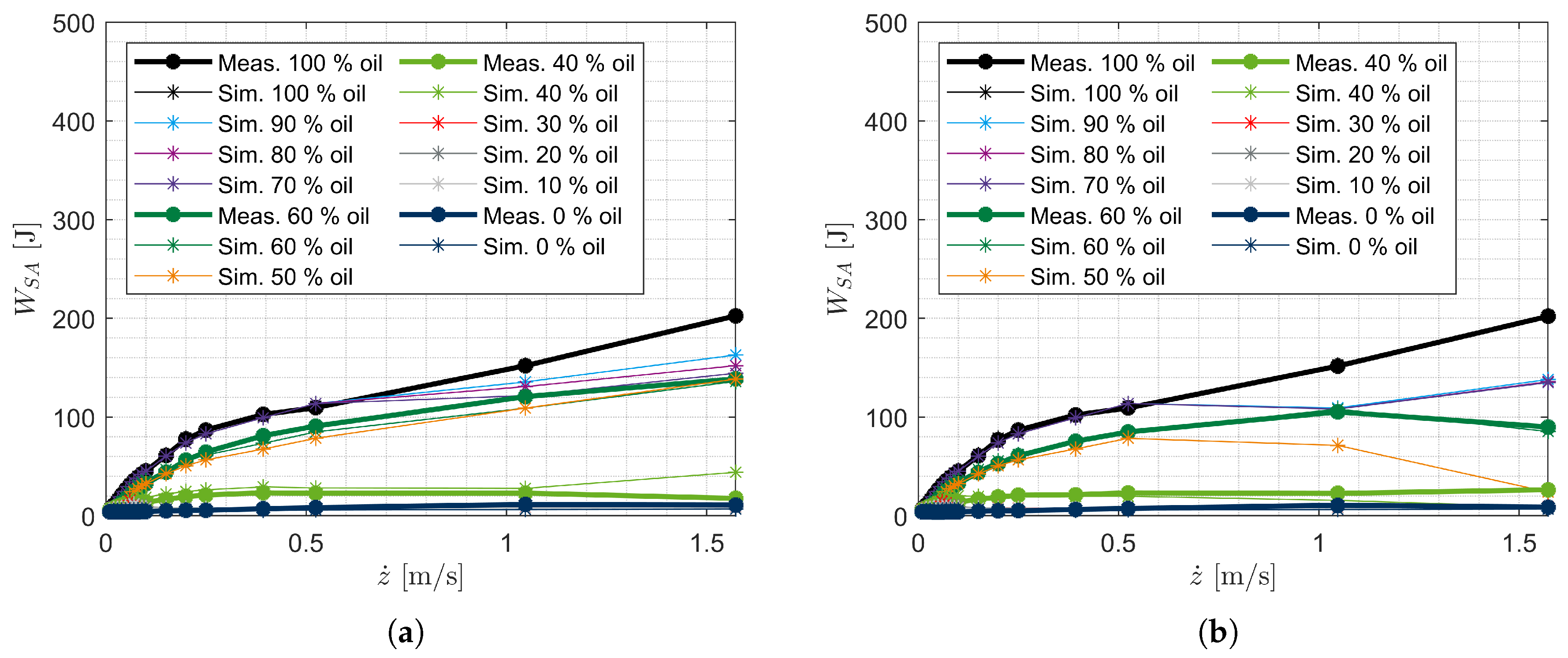
Table 2.
Shock absorber conditions
| Shock absorber | 1 | 2 | ||||||
| Condition [%] | 100 | 60 | 40 | 0 | 100 | 60 | 40 | 0 |
| Real oil volume [ml] | 321 | 161 | 112 | 0 | 264 | 166 | 106 | 0 |
| Real oil proportion [%] | 100 | 50 | 35 | 0 | 100 | 63 | 40 | 0 |
| Shock absorber | 3 | 4 | ||||||
| Condition [%] | 100 | 60 | 40 | 0 | 100 | 60 | 40 | 0 |
| Real oil volume [ml] | 371 | 226 | 148 | 0 | 239 | 160 | 96 | 0 |
| Real oil proportion [%] | 100 | 61 | 40 | 0 | 100 | 67 | 40 | 0 |
| Shock absorber | 5 | 6 | ||||||
| Condition [%] | 100 | 60 | 40 | 0 | 100 | 60 | 40 | 0 |
| Real oil volume [ml] | 332 | 239 | 133 | 0 | 153 | 95 | 61 | 0 |
| Real oil proportion [%] | 100 | 72 | 40 | 0 | 100 | 62 | 40 | 0 |
| Shock absorber | 7 | 8 | ||||||
| Condition [%] | 100 | 60 | 40 | 0 | 100 | 60 | 40 | 0 |
| Real oil volume [ml] | 354 | 194 | 114 | 0 | 273 | 153 | 83 | 0 |
| Real oil proportion [%] | 100 | 55 | 32 | 0 | 100 | 56 | 30 | 0 |
Table 3.
Measurement plan
| No. | Measurement |
|---|---|
| 1 | Quasi-static measurements |
| 2 | Harmonic measurements |
| 3 | Speed bump crossing 8 km/h |
| 4 | Cleat crossings 4 km/h |
| 5 | Cleat crossings 20 km/h |
| 6 | Cleat crossings 40 km/h |
| 7 | Uneven road washboard 4 km/h |
| 8 | Uneven road braking manoeuvre from 30 km/h |
| 9 | Uneven road braking manoeuvre from 50 km/h |
| 10 | Uneven road drive 4 km/h |
| 11 | Uneven road drive 30 km/h |
| 12 | Uneven road drive 50 km/h |
Table 5.
Shock absorber dimensions
| Dimensions [mm] | SA 1 | SA 2 | SA 3 | SA 4 | SA 5 | SA 6 | SA 7 | SA 8 |
| 45.50 | 41.20 | 50.20 | 41.20 | 46.60 | 38.00 | 50.00 | 41.40 | |
| 22.00 | 13.00 | 25.00 | 13.00 | 25.00 | 14.00 | 25.00 | 13.00 | |
| 32.00 | 29.90 | 35.90 | 30.00 | 36.00 | 27.00 | 35.80 | 29.80 | |
| 34.80 | 32.00 | 38.65 | 32.00 | 38.60 | 29.00 | 38.60 | 32.10 | |
| 326.00 | 277.90 | 326.00 | 277.90 | 328.00 | 225.70 | 326.00 | 331.00 |
Table 6.
Model parameter definition part 1
| Parameter | Definition |
| Oil proportion that flows through the PV simultaneously | |
| with gas during rebound | |
| Leakage factor; proportion of oil that flows through the | |
| PV without generating a damping force | |
| Proportion of the oil that flows through the PV and not | |
| through the BV during the compression stroke | |
| Oil proportion that flows through the PV simultaneously | |
| with gas during compression stroke | |
| Oil flow proportion from through the PV in relation | |
| to the total oil outflow from in the compression | |
| stage when is completely filled with oil |
Table 7.
Model parameter definition part 2
| Parameter | Definition |
| Proportion of the gas volume flow through the BV, | |
| which is converted into foam during the rebound stroke | |
| Oil proportion of the foam that is generated in the BV during | |
| the rebound stroke | |
| Proportion of the gas volume flow through the PV, | |
| which is converted into foam during the compression stroke | |
| Oil proportion of the foam that is formed in the PV during | |
| the compression stroke | |
| B | Properties of the foam more like oil (B=1) |
| or gas (B=0) | |
| E | Relationship between oil proportion of the foam |
| and damping force |
Table 8.
Model parameter definition part 3
| Parameter | Definition |
| Cavitation model treshold velocity | |
| Oil proportion which is transformed into gas during compression | |
| Oil proportion which is transformed into gas during rebound |
Disclaimer/Publisher’s Note: The statements, opinions and data contained in all publications are solely those of the individual author(s) and contributor(s) and not of MDPI and/or the editor(s). MDPI and/or the editor(s) disclaim responsibility for any injury to people or property resulting from any ideas, methods, instructions or products referred to in the content. |
© 2025 by the authors. Licensee MDPI, Basel, Switzerland. This article is an open access article distributed under the terms and conditions of the Creative Commons Attribution (CC BY) license (http://creativecommons.org/licenses/by/4.0/).
Copyright: This open access article is published under a Creative Commons CC BY 4.0 license, which permit the free download, distribution, and reuse, provided that the author and preprint are cited in any reuse.


