Submitted:
25 March 2025
Posted:
26 March 2025
Read the latest preprint version here
Abstract
We investigate the fully relativistic spherical collapse model of a uniform distribution of mass $M$ with initial comoving radius $\chi_*$ and spatial curvature $k \equiv 1/\chi_k^2 \le 1/\chi_*^2$ representing an over-density or bounded perturbation within a larger background. Our model incorporates a perfect fluid with an evolving equation of state, $P = P[\rho]$, which asymptotically transitions from pressureless dust ($P = 0$) to a ground state characterized by a uniform, time-independent energy density $\rho_{\rm G}$. This transition is motivated by the quantum exclusion principle, which prevents singular collapse, as observed in supernova core-collapse explosions. We analytically demonstrate that this transition induces a gravitational bounce at a radius $R_{\rm B} = (8 \pi G \rho_{\rm G}/3)^{-1/2}$. The bounce leads to an exponential expansion phase, where $P[\rho]$ behaves effectively as an inflation potential. This model provides novel insights into black hole interiors and, when extended to a cosmological setting, predicts a small but non-zero closed spatial curvature: $ -0.07 \pm 0.02 \le \Omega_k < 0$. This lower bound follows from the requirement of $\chi_k \ge \chi_* \simeq 15.9$ Gpc to address the cosmic microwave background low quadrupole anomaly. The bounce remains confined within the initial gravitational radius $r_{\rm S} = 2GM$, which effectively acts as a cosmological constant $\Lambda$ inside $r_{\rm S}=\sqrt{3/\Lambda}$ while still appearing as a Schwarzschild black hole from an external perspective. This framework unifies the origin of inflation and dark energy, with its key observational signature being the presence of a small, but nonzero, spatial curvature, a testable prediction for upcoming cosmological surveys.
Keywords:
cosmology
; theory
; inflation
; early Universe
; dark energy
; black hole physics
1. Introduction
The standard model of cosmology, rooted in the Big Bang paradigm and the theory of General Relativity (GR) with the addition of cosmological constant () and cold dark matter (CDM), has been remarkably successful in explaining key observations, such as the Cosmic Microwave Background (CMB), the large-scale structure of the Universe, and the accelerating cosmic expansion attributed to dark energy. However, several fundamental questions remain unresolved, such as the nature of the initial singularity, the flatness and horizon problems (or the origin of inflation), and the physical origin of dark energy. These challenges have spurred the development of alternative frameworks that seek to extend or complement the standard cosmological model. The nature of CDM and the origin of the smallness of the have been the central issues of modern cosmology.
A related problem is that of understanding the singular collapse into a Black Hole. Both problems can be addressed when we consider the relativistic spherical collapse of a local (finite) FLRW cloud within a larger background, as shown in Figure 1. A cosmological bounce and an inflationary phase can emerge naturally from two fundamental assumptions: and , which simply follow from considering a finite over-density of matter obeying the quantum exclusion principle, which prevents the density from overcoming some threshold value or ground state .
Crucially, this quantum mechanism violates the strong energy condition (SEC) in classical GR. As was shown in [1], the bounce requires a non-zero local curvature . Both conditions sidestep the singularity GR theorems proposed by [2], allowing us to formulate a novel solution to a pivotal issue in cosmological theory.
The bouncing scenario we formulate naturally extends to the subsequent stage of inflationary expansion when spatial curvature effects become negligible, resulting in the resolution of the horizon and flatness problems. Since the model is confined to a finite comoving region of spacetime, it introduces a finite comoving cutoff for super-horizon perturbations, potentially explaining anomalies in the CMB, such as the absence of structures beyond 66 degrees [3]. This is a unique aspect of the model that is actually compatible with CMB observations, unlike the standard framework of inflationary cosmology. The value of this cut-off directly relates to a prediction of spatial curvature .
A recent paper ([1]) has numerically solved the Newtonian spherical collapse equations with a polytropic equation of state (EoS) inspired by neutron star (NS) conditions. It found bounces at or above nuclear saturation density with equivalent GR behavior in a closed FLRW metric. The GR bounce corresponds to the ground state of the matter, characterized by (which is often termed a meta-stable state or quasi-deSitter in the framework of standard inflation). Here, we elaborate on the underlying mechanisms of this phenomenon and its implications for cosmic evolution, and we find new analytical and numerical solutions for the bounce, which are fully relativistic and within classical GR with a perfect fluid .
Our approach relates closely to [4,5,6], who studied the full general relativistic problem of a uniform and finite FLRW fluid ball (also called patch or cloud) expanding or contracting in a surrounding Schwarzschild vacuum. The contracting balls with pressure were also considered by Thompson and Whitrow [7] and Bondi [8], mainly to study gravitational collapse to black holes. Smoller and Temple [9] consider exact solutions of the Einstein equations representing spherical shock waves that extend the Oppenheimer-Snyder model [10] to the case of nonzero pressure inside the black hole.
Our approach is also related to cosmological bouncing scenarios (such as [11,12,13,14,15,16]) with some critical distinctions. Unlike other approaches, which modify gravity or try to quantize matter to explain the bounce, we find a solution for a perfect fluid EoS within standard GR, which is analogous to an effective scalar field in standard cosmic inflation models. It is worth noting here that when we include quantum effects in curved spacetime, even if we initially start with classical fluid with positive pressure, one gets negative pressure contributions as is shown in the studies of semi-classical gravity [17,18,19]. The quantum exclusion principle sets a new universal goal for the theories of quantum gravity [20,21,22]. Although the full study of quantum gravity is beyond the scope of this current study, it lays a foundation for what the actual theory of quantum gravity is supposed to achieve or to be consistent with. However, a pre-requirement for a complete theory of quantum gravity is the robust development of quantum field theory in curved spacetime [23,24,25], which we aim to develop in the future for the non-singular origin of the Universe we present here.
The FLRW cloud bounce and subsequent inflation are driven by the degenerate pressure , and this is supported by the hypothesis of the quantum exclusion principle, i.e., GR with quantum matter avoids singularities, which aligns very well with Misner’s thoughts on how quantum theory should avoid singularities [26]. A new key ingredient for our approach is to consider a finite cloud, which allows us to incorporate spatial curvature, demonstrating its essential role in enabling the bounce. Finally, we address how cosmic acceleration emerges as a natural consequence of the bounce.
This work stands on its own, but it can also be used to extend and complement the Black Hole Universe (BHU) model ([27,28]) with a closed FLRW cloud . The flat case used previously is a good approximation all the way to the point where we approach the singularity but does not allow for a bounce to occur. By connecting the early and late phases of cosmic evolution, it provides a unified model that bridges gravitational collapse, cosmic inflation, and the present accelerated expansion of the Universe. Grounded in physical principles and supported by numerical simulations, this model offers a compelling alternative to the standard cosmological paradigm while addressing its unresolved challenges. We use except when otherwise stated.
2. Spherical Collapse
Here, we want to model the collapse of a finite cloud or perturbation within a larger background. We will assume that the initial cloud is a spherical overdense region of a perfect fluid that is surrounded by an empty space, as shown in Figure 1. This configuration is embedded in a larger volume containing a homogeneous, more diluted fluid. We also assume that or negligible to start with. For an observer moving with a perfect fluid, the energy-momentum tensor is diagonal: , where is the relativistic energy density and is the pressure. The cloud is initially very large and has a very low density, so the pressure and temperature can be neglected. The relativistic solution to this problem was given by [29] `atom universe’ and is known today as the Lemaitre-Tolman-Bondi (LTB) model. The most general spherically symmetric metric in the comoving frame (i.e., moving with the fluid) is:
where with . The physical radius (or aerial coordinate) corresponds to the area distance and reflects spherical symmetry. The functional form of results from in the comoving frame. The general solution to the Einstein field equation is:
where the over dots correspond to partial time derivatives. The mass-energy M was introduced by [29] and is sometimes called the active gravitational mass and coincides with the relativistic Misner-Sharp mass ([30]), which is defined for the more general case with pressure [31].
Assuming a homogeneous cloud requires H to also be homogeneous. Consequently, and k has to be constant. We then have:
where and are the initial density and comoving radius of the cloud so that the mass m inside remains constant. Note that we use comoving units such that at present. This is the same solution as the FLRW solution, as expected. In general, we can choose k to have any sign depending on the initial conditions. The case of interest here is with , which corresponds to an overdensity. The value of relates to the initial velocity of the cloud when :
This reproduces the well-known result that a closed FLRW model exactly reproduces the relativistic spherical collapse model (see §87 in [32]). In the Newtonian approximation, positive curvature () corresponds to a system with negative total energy, where gravitational attraction exceeds kinetic energy, leading to the collapse of the cloud under its own gravity. In GR, spatial curvature provides the geometric representation of a gravitationally bound system. Just as a bound orbit in Newtonian gravity (like a planet around a star) is confined, a closed universe (or a collapsing region) in GR is “confined” by its own curvature. The metric of our initial perturbation for is therefore the same as the one of a closed FLRW metric:
Note that because is cosmologically large, the corresponding curvature term is subdominant until . The solutions in Eqs.5-, and also for Eqs.2-, with are the same as those in the Newtonian collapse studied in [1] (note that the corresponding Newtonian energy neglects the effects of k). The FLRW cloud is a local and finite LTB solution in contrast to the standard FLRW metric, which is usually assumed to be global and infinite.
What happens in the LTB solution for in the region of empty space surrounding R? [29] also found a solution to this question. In his §11, he shows how variables can be changed to transform the LTB solution into the static Schwarzschild metric. This change of variables corresponds to a frame that is not comoving with the fluid, just as in the case of the static version of the de-Sitter metric (i.e., see [33]). Another way to approach this question is to show that the FLRW metric matches the Schwarzschild metric without discontinuities. Two different versions of this approach were presented in [34] and in §12.5.1 in [35]. Such matching solution is what we call the FLRW cloud, which has the FLRW metric inside and the Schwarzschild metric outside ([36] also presented the case and for timelike and null junctions).
As the FLRW cloud collapses under its own gravity (), the outer physical radius shrinks and eventually crosses inside the corresponding Schwarzschild radius: . When this happens, the FLRW cloud becomes a BH. For the cosmological case, both and are very large, which means that the corresponding densities are very small (this is not the case for stellar masses). The density at a given time before the collapse to the singularity in the absence of any pressure is
This is the solution to Eq.5 when the spatial curvature term is neglected. If we take m to be as large as the mass of our observable Universe (), we find from Eq. that at horizon crossing: the density of the BH, is:
At these low densities, it is reasonable to assume that the thermal pressure P and temperature T are negligible because the time scale of the collapse is negligible compared to the time scales for any interactions between neutral particles. The cold collapse proceeds inside the BH event horizon. Note in Eq.9 how even up to one second before the singularity occurs, the density is small compared to nuclear saturation in a NS:
3. Spherical Collapse
The FLRW cloud solution for the general case of , where is the EoS, changes to:
where we have set for clarity. Even if is non-zero, its contribution can be neglected when we approach high densities.
4. Degeneracy Pressure
Here, we draw an analogy of our understanding of the Universe with NSs and astrophysical black holes. As the collapsing cloud approaches the singularity (), the density increases without bound. However, once any fermionic constituent of the cloud reaches its quantum ground state, the Pauli Exclusion Principle generates a degeneracy pressure, , independent of temperature. Remarkably, this degeneracy pressure and the corresponding equilibrium density apply universally to systems ranging from atoms to NS despite their vast difference in mass—approximately times. For even larger masses, such as the mass of the Universe (about times greater than that of a NS), the degeneracy pressures of electrons, neutrons, or even quarks may not suffice to halt the collapse. Indeed, for masses exceeding the Tolman–Oppenheimer–Volkoff (TOV) limit of 2–3 , a black hole forms, and the collapse proceeds within the event horizon, leaving the internal physics largely unexplored. A version of the Pauli Exclusion Principle should remain valid even under extreme conditions, as no two fermions can occupy the same quantum state. Thus, a new quantum ground state, characterized by a maximum density , could also emerge if electrons and quarks are not fundamental, preventing a true singularity. This notion lies at the heart of applying principles of quantum theory in the context of gravity, which offers a framework to circumvent singular collapse and explore the limits of physical laws in extreme conditions.
In the central regions of the collapsing cloud, where the bounce occurs, the pressure and density can be treated as approximately uniform in the comoving frame. The validity of this assumption was demonstrated in [1] using hydrodynamical simulations.
We can see from Eq. that as , the relativist pressure . Appendix A shows one way to understand this in terms of scalar fields, where the EoS plays the role of the scalar potential .
We can define a cloud radius from Eq.:
which corresponds to the radius of the cloud when it reaches if we neglect the effects of pressure. For the mass of the Universe and when assuming nuclear saturation density (SD) as a lower limit (Eq.11):
This value of represents the beginning of the transition into the ground state. The model transitions from a state of constant total energy-mass (with a uniform but evolving energy density) to a state of uniform and time-invariant energy density.
We have found that the quantum exclusion principle leads to a ground state where the relativistic equation of state (EoS) becomes: . This EoS is fundamentally distinct from the one typically considered under nuclear saturation in NSs. A key assumption for NS is that GR is negligible at scales of inter-quantum interactions. However, it is crucial to recognize that gravity is inherently nonlinear. The active mass-energy, as defined in Eq., includes not only matter but also gravitational energy, which can not be neglected. Notably, around the ground state, the active mass exhibits exponential growth or decay in the comoving frame, highlighting a purely gravitational effect. This behavior is also captured in the relativistic continuity equation (Eq.):
where we have included c to illustrate that the second term is purely relativistic and does not appear in the Newtonian equation. This equation demonstrates that once a constant density is reached, the EoS naturally transitions to (back in units of ). This behavior is not captured by Newtonian dynamics (or relativistic corrections) and is therefore not present in conventional EoS models for NS, emphasizing the necessity of considering relativistic effects in describing such ground states. In the Newtonian approach, the pressure only appears as a force in the Euler equation. The GR analog of the Euler equation (or its first integral) is the Hubble-Lemaitre law in Eq.12, which is independent of pressure. The two approaches come together when we combine the Euler equation with the continuity equation.
The other important difference between our comoving EoS and the NS modeling is that we are considering the collapse (and later expanding) phases and not a static solution. So, our EoS lives in the comoving frame, while NS EoS refers to a Newtonian rest frame. What does the relativistic EoS look like in the rest frame? This is presented in Appendix B.
5. Bouncing Solution
Bringing together the insights from the two previous sections, we can now explore what happens during the collapse of an FLRW cloud as it reaches its ground state density somewhere above nuclear saturation. For a constant , Eq.12- become:
This corresponds to a gravitational bounce ( and ) at:
Note how it is critical that (or ) to have a bounce before the singularity () occurs. The bounce is only possible because both and the cloud is finite (that is, and ). It is physically inconsistent to perceive a bouncing scenario in an infinite FLRW cloud. This is reflected above by the mathematical fact that an infinite FLRW cloud has no bounce. The existence of imposes a natural cutoff in the spectrum of super-horizon perturbations generated during collapse, bounce, or inflation. This cutoff shows up in the CMB sky as:
where Gpc is the comoving radial distance to the CMB for and km/s/Mpc. Strong evidence for such a cutoff has been known since COBE and confirmed by WMAP and Planck ([37,38,39]). [40] estimated the homogeneity scale to be:
which implies:
which is the Gaussian curvature scale. This interpretation predicts a value today () of:
which, for , is consistent with a critical reanalysis of the Planck Legacy 2018 data [41]. This result also agrees with a previous independent way of modeling the low quadrupole measured in the WMAP power spectrum [42]. The limits for above assume that the homogeneity scale is the result of only . This also explains the low quadrupole [40]. However, if the homogeneity scale or the low value of has a different origin, then the value of in the floating FLRW cloud could be smaller. Inflation preceded by a bounce requires , and this could be found in upcoming cosmic surveys, as indicated by the analysis in [41].
The exact solution to Eq. is:
where is the time to/from the bounce () with , and is the radius of the cloud when it bounces:
which happens to be the gravitational radius of the ground state .
6. Cosmic Inflation
The solution in Eq.24 corresponds to an exponential expansion (or collapse) after (or before) the bounce, leading to a de-Sitter phase, just as in standard cosmic inflation. As mentioned before, the EoS plays the role of the inflation potential, and the actual solution is quasi-de-Sitter as we approach the respective ground state of the matter.
As an example, we can take the following toy ansatz to interpolate from to :
where at the time when the density is half of and quantities with a star index (*) are given in units of . Eq.12 becomes:
Solving this numerically, we can obtain the exact equation of state , using Eq.. For single field inflation like Starobinsky: (where is the scalar spectral index) [43]. The current bound on the tensor-to-scalar ratio is ([44]). This solution corresponds to and is shown in Figure 2. The corresponding EoS follows:
which corresponds to the generalized Chaplygin gas with [45].
The ground state is approached asymptotically, with the density remaining constant even as the scale factor grows or decreases exponentially. This behavior arises because the active mass m is no longer constant, a purely relativistic effect where the gravitational field itself contributes non-linearly to the source term. Consequently, the model transitions from a regime of constant energy-mass, characteristic of a Newtonian solution, to one of constant energy-density, which is inherently relativistic.
As mentioned before, the saturation densities in NSs and the nucleus of an atom are comparable with Eq.11 despite the former having a mass times larger than the latter. However, as discussed in [1], the densities at which the condition is fulfilled for masses much larger than that observed for NSs could be significantly higher than that of Eq.11 so that the energy of the corresponding cosmic inflation could be much larger. In Appendix A, we show a more detailed comparison of with inflation parameters and CMB observations. The amplitude of CMB fluctuations relates to a ground state that has energy densities much larger than nuclear saturation. The quasi-scale invariant spectrum and quantum parity features observed in the CMB (see [46]) will also be reproduced with our bouncing solution.
In summary, a bounce driven by degeneracy pressure could give rise to an epoch of cosmic inflation and reheating. This opens the possibility for an epoch of nucleosynthesis and recombination similar to that in the standard model (e.g., see [47]). Note that in standard inflation, reheating requires an oscillatory scale factor around the matter-dominated phase after the exponential expansion, in typical single field inflation where M is inflaton mass. The equivalent process in terms of is detailed in Appendix A. This process has the potential to enable nucleosynthesis and recombination in a manner similar to the standard Big Bang model. More importantly, it also provides an alternative framework for understanding both early and late-time cosmic acceleration.
7. Cosmic Acceleration
There is compelling observational evidence that the cosmic expansion is accelerating: [48,49,50,51,52,53]. This acceleration appears to be dominated by the cosmological constant . The term can be interpreted as either a fundamental modification of General Relativity (GR), denoted as , or as an effective dark energy (DE) fluid, , analogous to the ground state described earlier, but with a much smaller energy density, .
Regardless of the interpretation, the corresponding characteristic length scale,
is vastly larger than the nuclear saturation scale (i.e., ). Consequently, can be neglected in our discussion of the gravitational bounce and the corresponding inflationary period.
The measured value of is extremely small but non-zero, and its fundamental origin remains an open question. Although its connection to the fundamental laws of physics is unclear, its effect is well understood: it induces an event horizon, , in FLRW space-time:
beyond which regions () are not causally connected to the interior (). The standard assumption in cosmology is that the universe beyond is identical to the interior. However, this assumption presents two fundamental issues:
- Lack of causal explanation: The standard approach cannot provide a mechanism to explain how the universe could be the same beyond . Cosmic inflation does not solve this puzzle because even under exponential expansion , we have that R is always . This is because the comoving distance travel by light during domination exactly cancels the exponential expansion in .
- Violation of the variational principle: Einstein’s field equations require that the metric asymptotically approaches Minkowski space at large distances, which is not satisfied if the universe extends indefinitely.
Instead, if we assume that the region beyond is empty, both of these issues are resolved. This leads to a finite universe with size and a finite total mass m contained within it. The exterior is then naturally described by the Schwarzschild metric. This agrees well with the FLRW cloud model presented here in previous sections and in Figure 1. For consistency, we need to identify with the Schwarzschild radius:
as both quantities are constant. This immediately provides a physical interpretation of :
Thus, simply corresponds to the total mass m of our finite universe. This also explains why is small but nonzero: it is directly linked to the total mass of the universe as in our FLRW cloud model. Thus, the measurement of a can be interpreted as a measurement of m and a confirmation that we live within a large, but finite FLRW cloud model. This is also consistent with our new interpretation of the origin of the bounce and cosmic inflation presented here.
This reasoning provides a straightforward and intuitive explanation of without requiring detailed calculations. Such calculations are presented in [36]. By applying the relevant matching conditions, it is found that the radial null geodesics satisfy Israel’s matching conditions and that the action principle correctly includes the extrinsic curvature boundary term, .
8. Discussion and Conclusion
This paper presents a novel solution to the relativistic spherical collapse model for a bounded perturbation (). The key innovation lies in the introduction of a variable equation of state, , which asymptotically evolves from a pressureless, homogeneous state to a ground state characterized by a time-independent energy density. This transition naturally gives rise to a de Sitter phase in the final stages of collapse—immediately preceding the bounce—and persists throughout the ensuing expansion. The bounce itself admits an analytical expression, provided in Eq. 24.
The cosmological implication of this new approach is a novel understanding of the origin of the universe that emerges from the collapse and subsequent bounce of a spherically symmetric matter distribution. We show that upon reaching a quantum ground state, the relativistic matter equation of state (EoS) transitions from to in the comoving frame. The relativistic degenerate pressure generated in this state halts the collapse and initiates a bounce and an inflationary expansion. We discussed how this mechanism parallels phenomena in NS physics and core-collapse supernovae (see reviews by [55,56,57,58]), where the ground state is determined by nucleonic or quark interaction potentials within proto-NS. On the other hand, the expansion mechanism right after the bounce also parallels with that of cosmic inflation as detailed in Appendix A.
The non-singular bounce that happens inside a closed FLRW cloud (i.e., a finite-sized Universe trapped inside an event horizon) is induced by quantum matter EoS, which results in degenerate negative pressure. This same process drives an exponential expansion analogous to cosmic inflation, offering a novel solution to key challenges in standard cosmology, such as the origin of inflation and dark energy. Our findings highlight the profound implications of relativistic quantum principles in shaping the early Universe.
We start from a low-density cloud with where is the adimensional scale factor in units of the value today . The key simplicity of this model is that the BH is not an ad-hoc initial condition to our system but a consequence of gravitational collapse. Without this, there is no argument for . This will happen for any initial condition where the initial density is sufficiently low. Harrison-Zeldovich-Peebles (1970) [59,60,61] independently argued that gravitational instability alone (without inflation) would naturally produce a scale-invariant spectrum of perturbations out of an FLRW metric. Such perturbations will give rise to overdensities such as the ones considered here as the starting point to our Universe. This is our new guess for the “initial condition".
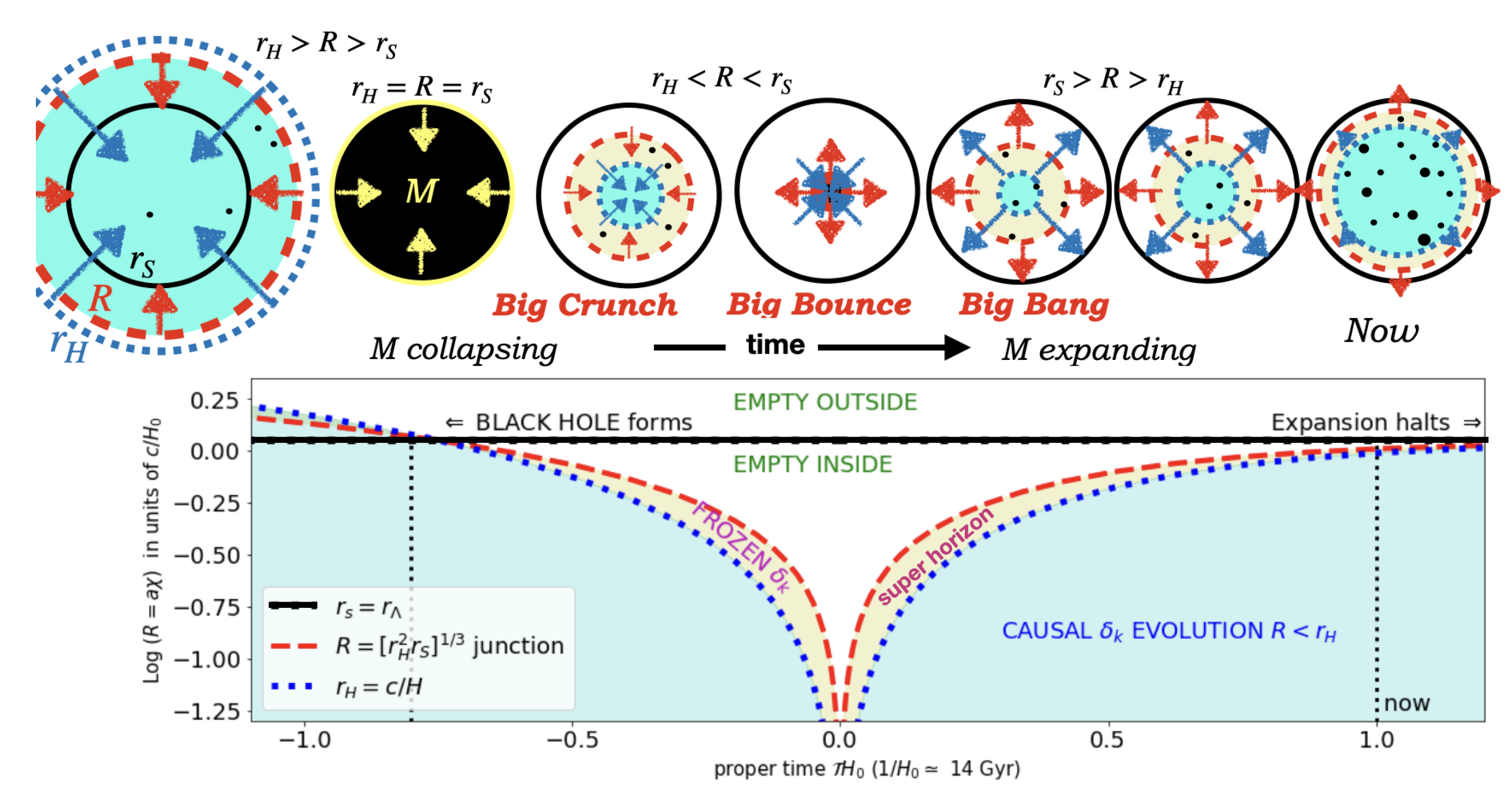
Figure 3 shows the full evolution of the finite FLRW cloud radius, , illustrating how the horizon problem is resolved within the bounce model. In the middle panel of Figure 2, we now present the exact bouncing solution, comparing the analytical expression for the scale factor given in Eq. 24 with the numerical solution of Eq. 27. For reference, we also plot the singular analytic solution for . Such singular behavior is unavoidable for an infinite cloud ( or ) or in a flat or open geometry (). Note how the inflationary phase has the right number of e-folds consistent with the scalar spectral index measured by Planck [43].
It is evident that the analytic solution in Eq. 24 is valid only for the inflationary phase, i.e., near the bounce, whereas the numerical solution accounts for the entire evolution, including the pre-bounce phase when . Before reaching the bounce, the numerical solution follows the pressureless analytic case closely, which is expected since the pressure is initially vanishing and then transitions smoothly into a constant (negative) degeneracy pressure (), as shown in the left panel. In this regime, the equation of state (EoS) is well approximated by (dashed line). When we plot the Pressure calculated for the numerical model (labeled ) as a function of the corresponding density and fit it, the fitting curve is with and . This can be interpreted as a polytropic EoS with .
Furthermore, the transition point is clearly marked: as soon as pressure begins to build up, the numerical solution in the middle panel shifts from the analytic solution (dotted line) to the analytic bounce solution (dashed line), denoting exponential collapse and vice-versa for exponential expansion.
The right panel provides a zoomed-in view of the bounce region, where we compare our asymptotic analytical solution with the numerical Newtonian simulations of [1], which adopt an equation of state of the form . This type of EoS serves as a reasonable approximation for nuclear degenerate matter, with to 3, in the Newtonian framework [62]. While the Newtonian simulations remain an approximation, we observe that both models yield a strikingly similar exponential expansion post-bounce, as also noted by [1]. Note that the Newtonian simulation results presented here are for a 20 M⊙ cloud, for which the bounce occurs at around nuclear saturation densities and the expansion has e-folds. For larger masses, we will have a larger number of e-folds as in the middle panel for the mass of our Universe.
The analytic solution we found in Eq.24 is one of the cases considered in Eq.7 in [12], which corresponds to a de-Sitter Universe with closed curvature. Instead of degeneracy pressure, this model arises from quadratic curvature modification of the Einstein-Hilbert action motivated by 1-loop self-energy contributions due to quantum matter, which leads to the first model of cosmic inflation ([63]). But the reason to consider closed curvature (other than to produce a bounce as in [11]) is not clear in this model. In the BHU model, the spatial curvature naturally results from the spherical collapse of a large overdensity confined to a finite region of spacetime.
Figure 3 in [36] illustrates how the boundary of the FLRW cloud is always outside the observational window for any (off-centered) observer inside the cloud. This is a general property of quasi-de-Sitter space and implies that the BHU does not result in observed anisotropies in the background of the cloud boundary. But the bounce and the initial cloud’s comoving radius can result in a cutoff of the super-horizon quantum perturbations generated during inflation, which can be observed in the CMB [3,40,64] and results in the constraint given by Eq.22. Such cutoff, together with parity asymmetry, predicts a lower quadrupole, which can explain several other CMB anomalies (see [25,46,65]).
Our analysis shows that the observed cosmological constant can be interpreted as a boundary effect from the gravitational radius of the BHU, aligning with the idea of an effective term without invoking exotic physics. The implications of this model extend to the generation of super-horizon perturbations, the observed entropy ratio of baryons to photons, and the potential origins of dark matter ([66]). Future studies should explore the role of temperature and radiation in nuclear fusion during the bounce to provide a more comprehensive understanding of the transition from collapse to expansion.
The smoking gun for our bouncing scenario is the presence of both a small spatial curvature and a small term. While the latter has already been measured with high precision, the former remains a testable prediction (given here in Eq. 23) for upcoming cosmological surveys. The Planck PR3 lensed power spectrum revealed a preference for positive curvature [67], with , in agreement with our Eq. 23. Recent results from ACT [68] similarly suggest a slight preference for positive curvature (see their Fig. 9), although the current uncertainties remain too large to decisively rule out a flat universe. The latest DESI data [69] echo this trend, also hinting at a mild preference for positive curvature. Together, the ACT and DESI results support a growing pattern: when multiple high-precision datasets are combined, persistent tensions with the standard CDM model begin to emerge. Notably, the combination of DESI and CMB data reveals evidence for a term that evolves slowly over cosmological time. In our framework, where , this corresponds to a decreasing FLRW cloud mass m over time. If confirmed, such behavior could be interpreted as a signature of quantum horizon effects—such as black hole evaporation via Hawking radiation [23,24,70]. Nonetheless, individual cosmological measurements have not yet yielded definitive evidence for departures from the standard CDM scenario.
Acknowledgments
EG acknowledges grants from Spain Plan Nacional (PGC2018-102021-B-100) and Maria de Maeztu (CEX2020-001058-M). KSK acknowledges the support from the Royal Society through the Newton International Fellowship. SP acknowledges the support and hospitality at the Institute of Cosmology and Gravitation during a 3-month stay to conclude his Master’s Thesis. MG acknowledges the support through the Generalitat Valenciana via the grant CIDEGENT/2019/031, the grant PID2021-127495NB-I00 funded by MCIN/AEI/10.13039/501100011033 and by the European Union, and the Astrophysics and High Energy Physics program of the Generalitat Valenciana ASFAE/2022/026 funded by MCIN and the European Union NextGenerationEU (PRTR-C17.I1).
Appendix A. Analogy with Scalar Field
We can model the quantum ground state of nuclear saturation by introducing a scalar degree of freedom . Consider the Einstein-Hilbert action with minimally coupled matter fields with Lagrangian :
where the last integral represents the Gibbons-Hawking-York (GHY) boundary term [71,72,73], and is the trace of the extrinsic curvature at the boundary . This term is needed in the cases where the manifold under study has some boundary (as happens inside a BH). The energy-momentum is defined as:
The least action principle with respect to the metric yields Einstein field equations:
where variations of the field are zero at the integration limits thanks to the GHY boundary term. For the Lagrangian, we consider a combination of a perfect fluid and an effective minimally coupled scalar field with: , where and is the standard matter-energy content. We have defined and is the potential of the classical scalar field . We will next explore the regime where is dominated by . If both and contributions are not coupled, then the general result would correspond to just adding both contributions to P and . We can estimate the contribution of the scalar field from equation (A2):
Choosing an observer that is moving with the fluid and comparing it to a perfect fluid, we can identify (see also equations B66-B68 in [74]):
where we have defined . The ground state of the system corresponds to the configuration in which the energy is minimized. In a relativistic context, this often means that the kinetic contributions (derived from the gradient terms ) become insignificant compared to the potential energy . This simply means that the total energy is dominated by the potential energy. We expect something similar to happen when the collapsing cloud reaches the ground state at some supra-nuclear densities in a cold collapse. The dynamics will be dominated by the potential of the interaction of quantum particles, and their kinetic energy will not play a significant role in the evolution at the bounce. Close to the ground state, . During its evolution, first, the cloud ascends (rolls up) towards the potential as it collapses, and after the bounce, it descends (rolls down). Analogously to the scalar field considered here, a fluid with a given EoS will reach some saturation density . Consequently, the EoS plays a role in the scalar potential.
If we take (Planck TT+TE+EE+LowE+Lensing) at from the Planck data [75]) we find (considering the spectral index derived for Starobinsky-like inflationary scenario [76]:
where are the slow-roll parameters that characterize the inflationary expansion after the bounce.
These are related to energy density and pressure EoS as (in the units of )
which are small during the inflationary expansion, which is followed by (quasi-de Sitter) bounce that occurs in our model due to negative degeneracy pressure. In the case of Starobinsky or Higgs inflation .
The primordial power spectrum (of curvature perturbation ) in the framework of single-field slow-roll inflationary models is
where is the pivot scale chosen by the Planck data, is the amplitude of the power spectrum, which at the pivot scale measured to be , is the value of Hubble parameter during inflation and is the known as slow-roll parameter that measures how slowly Hubble parameter varies during inflation. Using the observational constraint on the amplitude of the power spectrum, the Hubble parameter during inflation can be estimated to be
In the case of Starobinsky inflation which yields .
Although the above measurements are much smaller than the Planck values, they remain significantly larger than the nuclear saturation scale given in Eq. 11. This suggests the existence of a higher-energy ground state beyond neutral saturation. In particular, this energy scale is comparable to those typically considered in inflationary models, such as Starobinsky-like inflationary models [76]. Moreover, it aligns with the observed normalization of the CMB temperature power spectrum, , at the pivot scale , reinforcing its relevance in early-universe physics.
Appendix B. Relativistic EoS in the Rest Frame
Consider a change in variables from comoving coordinates to rest frame coordinates , where is the rest frame radial coordinate, while angular variables remain the same. The most general form for a metric with spherical symmetry can be written in terms of Bardeen potentials and as:
The FLRW comoving metric in Eq.8 transforms into the rest frame FLRW metric in Eq.A10 as:
where the angular part is the identity matrix. Explicitly:
where . The general solution to these equations is:
where is the Weyl potential, where is arbitrary and with . This frame duality can be interpreted as a Lorentz contraction where the velocity u is given by the Hubble-Lemaitre law: . An observer in the rest frame, not moving with the fluid, sees the moving fluid element contracted by the Lorentz factor : [33].
We can now use the inverse transformation, , in Eq. A14 to determine the energy-momentum tensor in the rest frame:
We observe that the off-diagonal terms are generally nonzero, indicating that the fluid is moving in the rest frame (), as expected. Furthermore, the stress-energy tensor is no longer uniform, even when P and are, implying that both the rest-frame relativistic pressure and energy density depend on time and radius, . At the center (), the energy density and pressure are the same in both frames, i.e., and . Neglecting the off-diagonal terms—corresponding to large values of , small u, or the near-degenerate case —we can explicitly express the radial dependence in terms of :
In the limit of degenerate pressure (the ground state), where , the energy density and pressure remain unchanged in both frames, i.e., and .
References
- Pradhan, S.; Gabler, M.; Gaztañaga, E. Cold collapse and bounce of an FLRW cloud. Monthly Notices of the Royal Astronomical Society 2025, 537, 1232–1248. [Google Scholar] [CrossRef]
- Hawking, S.W.; Penrose, R.; Bondi, H. The singularities of gravitational collapse and cosmology. Proc. of the Royal Society of London 1970, 314, 529–548. [Google Scholar]
- Gaztañaga, E.; Camacho-Quevedo, B. What moves the heavens above? Physics Letters B 2022, arXiv:astro-ph.CO/2204.10728]835, 137468. [Google Scholar] [CrossRef]
- Zel’Dovich, Y.B. Semiclosed Worlds in the General Theory of Relativity. Soviet Journal of Experimental and Theoretical Physics 1963, 16, 732. [Google Scholar]
- Geller, S.R.; Bloomfield, J.K.; Guth, A.H. Mass of a Patch of an FRW Universe. arXiv e-prints 2018, arXiv:1801.02249. [Google Scholar] [CrossRef]
- Faraoni, V.; Atieh, F. Turning a Newtonian analogy for FLRW cosmology into a relativistic problem. Phys. Rev. D 2020, 102, 044020. [Google Scholar] [CrossRef]
- Thompson, I.H.; Whitrow, G.J. Time-dependent internal solutions for spherically symmetrical bodies in general relativity-II. Adiabatic radial motions of uniformly dense spheres. MNRAS 1968, 139, 499. [Google Scholar] [CrossRef]
- Bondi, H. Gravitational bounce in general relativity. MNRAS 1969, 142, 333. [Google Scholar] [CrossRef]
- Smoller, J.; Temple, B. Shock-wave cosmology inside a black hole. Poceedings of the NAS 2003, 100, 11216–11218. [Google Scholar] [CrossRef]
- Oppenheimer, J.R.; Snyder, H. On Continued Gravitational Contraction. Physical Review 1939, 56, 455–459. [Google Scholar] [CrossRef]
- Starobinskii, A.A. On a nonsingular isotropic cosmological model. Pisma v Astronomicheskii Zhurnal 1978, 4, 155–159. [Google Scholar]
- Starobinsky, A.A. A new type of isotropic cosmological models without singularity. Physics Letters B 1980, 91, 99–102. [Google Scholar] [CrossRef]
- Brandenberger, R.; Peter, P. Bouncing Cosmologies: Progress and Problems. Foundations of Physics 2017, arXiv:hep-th/1603.05834]47, 797–850. [Google Scholar] [CrossRef]
- Nojiri, S.; Odintsov, S.D.; Oikonomou, V.K. Modified gravity theories on a nutshell: Inflation, bounce and late-time evolution. PhysRep 2017, arXiv:gr-qc/1705.11098]692, 1–104. [Google Scholar] [CrossRef]
- Odintsov, S.D.; Oikonomou, V.K.; Fronimos, F.P.; Fasoulakos, K.V. Unification of a bounce with a viable dark energy era in Gauss-Bonnet gravity. 10402020; 102, 104042arXiv:gr-qc/2010.13580]. [Google Scholar] [CrossRef]
- Kiefer, C.; Mohaddes, H. Quantum theory of the Lemaitre model for gravitational collapse. General Relativity and Gravitation 2025, 57, 26. [Google Scholar] [CrossRef]
- Cesar e Silva, W.; Shapiro, I.L. Semiclassical bounce with strong minimal assumptions. Phys. Rev. D 2024, arXiv:gr-qc/2402.18785]110, 043540. [Google Scholar] [CrossRef]
- Cesar e Silva, W.; Oliveira, S.W.P.; Shapiro, I.L. Bounce solutions with quantum vacuum effects of massive fields and subsequent Starobinsky inflation. 2 arXiv:gr-qc/2502.02281], 2025.
- Shapiro, I.L. Effective Action of Vacuum: Semiclassical Approach. Class. Quant. Grav. 2008, arXiv:gr-qc/0801.0216]25, 103001. [Google Scholar] [CrossRef]
- Loll, R.; Fabiano, G.; Frattulillo, D.; Wagner, F. Quantum Gravity in 30 Questions. PoS 2022, arXiv:hep-th/2206.06762]CORFU2021, 316. [Google Scholar] [CrossRef]
- Buoninfante, L.; etal., *!!! REPLACE !!!*. Visions in Quantum Gravity. arXiv e-prints, 2024; arXiv:2412.08696. [Google Scholar] [CrossRef]
- Buoninfante, L.; Kumar, K.S. Quantum gravity, higher derivatives and nonlocality. Nuovo Cim. C 2022, 45, 25. [Google Scholar] [CrossRef]
- Kumar, K.S.; Marto, J. Towards a unitary formulation of quantum field theory in curved spacetime: the case of de Sitter spacetime. Symmetry 2025, arXiv:hep-th/2305.06046]17, 29. [Google Scholar] [CrossRef]
- Kumar, K.S.; Marto, J. Towards a Unitary Formulation of Quantum Field Theory in Curved Space-Time: The Case of the Schwarzschild Black Hole. PTEP 2024, arXiv:hep-th/2307.10345]2024, 123E01. [Google Scholar] [CrossRef]
- Gaztañaga, E.; Sravan Kumar, K.; Marto, J. A New Understanding of Einstein-Rosen Bridges. preprint, 2024; 2836794. [Google Scholar]
- Misner, C.W. Absolute zero of time. Phys. Rev. 1969, 186, 1328–1333. [Google Scholar] [CrossRef]
- Gaztañaga, E. How the Big Bang Ends Up Inside a Black Hole. Universe 2022, arXiv:astro-ph.CO/2204.11608]8, 257. [Google Scholar] [CrossRef]
- Gaztañaga, E. The mass of our observable Universe. MNRAS 2023, 521, L59–L63. [Google Scholar] [CrossRef]
- Lemaitre, G. The expanding universe. Annales Soc. Sci. Bruxelles A 1933, 53, 51–85. [Google Scholar] [CrossRef]
- Misner, C.W.; Sharp, D.H. Relativistic Equations for Adiabatic, Spherically Symmetric Gravitational Collapse. Phys. Rev. 1964, 136, B571–B576. [Google Scholar] [CrossRef]
- Faraoni, V. Lemaître model and cosmic mass. General Relativity and Gravitation 2015, arXiv:gr-qc/1506.06358]47, 84. [Google Scholar] [CrossRef]
- Peebles, P.J.E. The large-scale structure of the universe; 1980.
- Gaztañaga, E. On the Interpretation of Cosmic Acceleration. Symmetry 2024, 16, 1141. [Google Scholar] [CrossRef]
- Stuckey, W.M. The observable universe inside a black hole. American Journal of Physics 1994, 62, 788–795. [Google Scholar] [CrossRef]
- Padmanabhan, T. Gravitation, Cambridge Univ. Press; 2010.
- Gaztañaga, E. The Black Hole Universe, Part I. Symmetry 2022, 14, 1849. [Google Scholar] [CrossRef]
- Hinshaw, G.; etal., *!!! REPLACE !!!*. Two-Point Correlations in the COBE DMR Four-Year Anisotropy Maps. ApJl 1996, 464, L25. [Google Scholar] [CrossRef]
- Spergel, D.N.; etal., *!!! REPLACE !!!*. First-Year Wilkinson Microwave Anisotropy Probe (WMAP) Observations: Determination of Cosmological Parameters. ApJs 2003, 148, 175–194. [Google Scholar] [CrossRef]
- Planck Collaboration. Planck 2018 results. VII. Isotropy and statistics of the CMB. A&A 2020, arXiv:astro-ph.CO/1906.02552]641, A7. [Google Scholar] [CrossRef]
- Camacho-Quevedo, B.; Gaztañaga, E. A measurement of the scale of homogeneity in the early Universe. JCAP 2022, 2022, 044. [Google Scholar] [CrossRef]
- Di Valentino, E.; Melchiorri, A.; Silk, J. Planck evidence for a closed Universe and a possible crisis for cosmology. Nature Astronomy 2020, arXiv:astro-ph.CO/1911.02087]4, 196–203. [Google Scholar] [CrossRef]
- Efstathiou, G. Is the low cosmic microwave background quadrupole a signature of spatial curvature? MNRAS 2003, 343, L95–L98. [Google Scholar] [CrossRef]
- Planck Collaboration. Planck 2013 results. XXII. Constraints on inflation. A&A 2014, arXiv:astro-ph.CO/1303.5082]571, A22. [Google Scholar] [CrossRef]
- Galloni, G.; Bartolo, N.; Matarrese, S.; Migliaccio, M.; Ricciardone, A.; Vittorio, N. Updated constraints on amplitude and tilt of the tensor primordial spectrum. JCAP 2023, arXiv:astro-ph.CO/2208.00188]04, 062. [Google Scholar] [CrossRef]
- Multamäki, T.; Manera, M.; Gaztañaga, E. Large scale structure and the generalized Chaplygin gas as dark energy. 2004; 69, 023004arXiv:astro-ph/astro-ph/0307533. [Google Scholar] [CrossRef]
- Gaztañaga, E.; Sravan Kumar, K. Finding origins of CMB anomalies in the inflationary quantum fluctuations. JCAP 2024, arXiv:astro-ph.CO/2401.08288]2024, 001. [Google Scholar] [CrossRef]
- Steigman, G. Primordial Nucleosynthesis in the Precision Cosmology Era. ARNPS 2007, 57, 463–491. [Google Scholar] [CrossRef]
- Riess, A.G.; etal., *!!! REPLACE !!!*. Observational Evidence from Supernovae for an Accelerating Universe and a Cosmological Constant. AJ 1998, 116, 1009–1038. [Google Scholar] [CrossRef]
- Schmidt, B.P.; etal., *!!! REPLACE !!!*. The High-Z Supernova Search: Measuring Cosmic Deceleration and Global Curvature of the Universe Using Type Ia Supernovae*. The Astrophysical Journal 1998, 507, 46. [Google Scholar] [CrossRef]
- Perlmutter, S.; etal., *!!! REPLACE !!!*. Measurements of Ω and Λ from 42 High-Redshift Supernovae. The Astrophysical Journal 1999, 517, 565. [Google Scholar] [CrossRef]
- Fosalba, P.; Gaztañaga, E.; Castander, F.J. Detection of the Integrated Sachs-Wolfe and Sunyaev-Zeldovich Effects from the Cosmic Microwave Background-Galaxy Correlation. ApJL 2003, 597, L89–L92. [Google Scholar] [CrossRef]
- Eisenstein, D.J.; etal., *!!! REPLACE !!!*. Detection of the Baryon Acoustic Peak in the Large-Scale Correlation Function of SDSS Luminous Red Galaxies. The Astrophysical Journal 2005, 633, 560. [Google Scholar] [CrossRef]
- Betoule, M. .; etal. Improved cosmological constraints from a joint analysis of the SDSS-II and SNLS supernova samples***. A&A 2014, 568, A22. [Google Scholar] [CrossRef]
- DESI Collaboration.; etal. DESI 2024 VI: Cosmological Constraints from the Measurements of Baryon Acoustic Oscillations. arXiv e-prints 2024, p. arXiv:2404.03002, [arXiv:astro-ph.CO/2404.03002]. https://doi.org/10.48550/arXiv.2404.03002.
- Bethe, H.A. Supernova mechanisms. Reviews of Modern Physics 1990, 62, 801–866. [Google Scholar] [CrossRef]
- Burrows, A.; Hayes, J.; Fryxell, B.A. On the Nature of Core-Collapse Supernova Explosions. 1995, 450, 830, [arXiv:astro-ph/astro-ph/9506061]. [CrossRef]
- Hebeler, K.; Lattimer, J.M.; Pethick, C.J.; Schwenk, A. EQUATION OF STATE AND NEUTRON STAR PROPERTIES CONSTRAINED BY NUCLEAR PHYSICS AND OBSERVATION. ApJ 2013, 773, 11. [Google Scholar] [CrossRef]
- Janka, H.T.; Hanke, F.; Hüdepohl, L.; Marek, A.; Müller, B.; Obergaulinger, M. Core-collapse supernovae: Reflections and directions. Progress of Theoretical and Experimental Physics 2012, arXiv:astro-ph.SR/1211.1378]2012, 01A309. [Google Scholar] [CrossRef]
- Harrison, E.R. Fluctuations at the Threshold of Classical Cosmology. PRD 1970, 1, 2726–2730. [Google Scholar] [CrossRef]
- Zel’Dovich, Y.B. Gravitational instability: an approximate theory for large density perturbations. AAP 1970, 500, 13–18. [Google Scholar]
- Peebles, P.J.E.; Yu, J.T. Primeval Adiabatic Perturbation in an Expanding Universe. ApJ 1970, 162, 815. [Google Scholar] [CrossRef]
- Lattimer, J.M.; Prakash, M. Neutron star observations: Prognosis for equation of state constraints. PhysRep 2007, 442, 109–165. [Google Scholar] [CrossRef]
- Starobinskii, A.A. Spectrum of relict gravitational radiation and the early state of the universe. ZhETF Pisma Redaktsiiu 1979, 30, 719–723. [Google Scholar]
- Fosalba, P.; Gaztañaga, E. Explaining cosmological anisotropy: evidence for causal horizons from CMB data. MNRAS 2021, 504, 5840–5862. [Google Scholar] [CrossRef]
- Gaztañaga, E.; Sravan Kumar, K. Unitary quantum gravitational physics and the CMB parity asymmetry. arXiv 2024, arXiv:2403.05587, p. [Google Scholar] [CrossRef]
- Gaztañaga, E. The Black Hole Universe, Part II. Symmetry 2022, 14, 1984. [Google Scholar] [CrossRef]
- Planck Collaboration. Planck 2018 results. VI. Cosmological parameters. A&A 2020, arXiv:astro-ph.CO/1807.06209]641, A6. [Google Scholar] [CrossRef]
- ACT Collaboration. The Atacama Cosmology Telescope: DR6 Power Spectra, Likelihoods and ΛCDM Parameters. arXiv e-prints, arXiv:2503arXiv:astro-ph.CO/2503.14452. [CrossRef]
- DESI Collaboration. DESI DR2 Results II: Measurements of Baryon Acoustic Oscillations and Cosmological Constraints. arXiv e-prints 2025, p. arXiv:2503.14738, [arXiv:astro-ph.CO/2503.14738].
- Hawking, S.W. Particle creation by black holes. Communications in Mathematical Physics 1975, 43, 199–220. [Google Scholar] [CrossRef]
- York, J.W. Role of Conformal Three-Geometry in the Dynamics of Gravitation. Phy.Rev.Lett. 1972, 28, 1082–1085. [Google Scholar] [CrossRef]
- Gibbons, G.W.; Hawking, S.W. Cosmological event horizons, thermodynamics, and particle creation. PRD 1977, 15, 2738–2751. [Google Scholar] [CrossRef]
- Hawking, S.W.; Horowitz, G.T. The gravitational Hamiltonian, action, entropy and surface terms. Class Quantum Gravity 1996, 13, 1487. [Google Scholar] [CrossRef]
- Weinberg, S. Cosmology, Oxford University Press; 2008.
- Akrami, Y.; et al. Planck 2018 results. X. Constraints on inflation. Astron. Astrophys. 2020, arXiv:astro-ph.CO/1807.06211]641, A10. [Google Scholar] [CrossRef]
- Kehagias, A.; Moradinezhad Dizgah, A.; Riotto, A. Remarks on the Starobinsky model of inflation and its descendants. Phys. Rev. D 2014, 89, 043527. [Google Scholar] [CrossRef]
Figure 1.
Graphical representation of the spherical collapse. There are three uniform spherically symmetric distributions: (i) outer background , (ii) inner region with radius less than R and larger mean density , and (iii) empty space outside R. Two key ingredients of this configuration: a) the inner region collapse is decoupled from the background, and b) such gravitational bounded collapse is modeled in GR with a global spatial curvature .
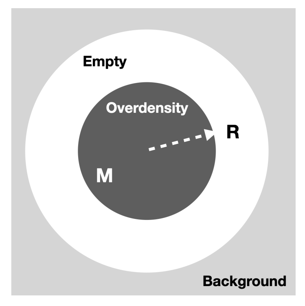
Figure 2.
The left panel shows the EoS (, blue, and , cyan) in units of , derived using the numerical solution of Eq.27 and Eq.. These are compared with from the case (black dotted) and the polytropic fit (dashed magenta). The middle panel shows a comparison of the different solutions for scale factor—the analytic solution presented in Eq.24, the numerical solution of Eq.27 for 57 e-folds of inflation, and the singular pressureless solution denoted with dashed, solid and dotted lines respectively. The right panel shows a zoom-in around the bouncing region, where we compare the analytical bounce solution in Eq.24 and the full numerical solution for in Eq.28 for 1.2 e-folds, with the Newtonian numerical simulations ([1]), with different polytropic EoS for nuclear saturation in NSs: with .
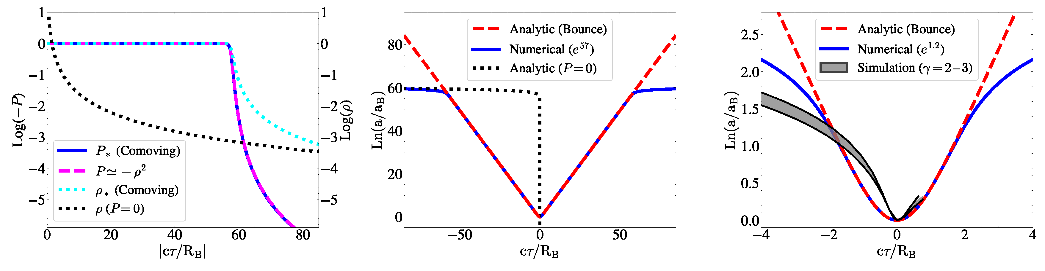
Figure 3.
The time evolution in the radius of the FLRW cloud , first forming a BH and then bouncing inside to form our current observed expanding Universe. The black circle represents the FLRW cloud gravitational radius, which is also the asymptotic event horizon of our current expansion. The dash-red and dot-blue lines and circles correspond to the FLRW cloud radius and the Hubble radius . This figure has been adapted from [27]. Licensed under CC-BY.
Disclaimer/Publisher’s Note: The statements, opinions and data contained in all publications are solely those of the individual author(s) and contributor(s) and not of MDPI and/or the editor(s). MDPI and/or the editor(s) disclaim responsibility for any injury to people or property resulting from any ideas, methods, instructions or products referred to in the content. |
© 2025 by the authors. Licensee MDPI, Basel, Switzerland. This article is an open access article distributed under the terms and conditions of the Creative Commons Attribution (CC BY) license (http://creativecommons.org/licenses/by/4.0/).
Copyright: This open access article is published under a Creative Commons CC BY 4.0 license, which permit the free download, distribution, and reuse, provided that the author and preprint are cited in any reuse.


