Submitted:
12 February 2025
Posted:
14 February 2025
Read the latest preprint version here
Abstract
Turbulence, by definition, arises from the interplay between fluid viscosity and velocity gradients. This insight prompted a re-examination of the foundational equations of fluid motion. The analysis reveals that the only arbitrary aspect in formulating these equations lies in the choice of the fluid's constitutive equation. The paper argues that, in turbulent flow, the substantial velocity gradients necessitate retaining second-order terms related to the deformation rate in the constitutive equation, which are often neglected. This retention leads to a more accurate constitutive equation for viscous fluids, enabling the derivation of hydrodynamic equations tailored for turbulent motion, free of adjustable parameters, and offering a refined modification of the Navier-Stokes equations.
Keywords:
Navier-Stokes equations
; turbulent flows
; constitutive equations
; velocity gradient
; boundary layers
1. Introduction
The mention of turbulence immediately brings to mind a saying: turbulence is one of the most challenging problems in physics and is known as an "unsolved problem in the classic physics." Historically, some renowned physicists and mathematicians, such as Werner Heisenberg, Richard Feynman, and Andrei Kolmogorov, dedicated their wonderful lives to the problem of turbulence without solving it. It is even said that the famous physicist Horace Lamb hoped to ask God about turbulence after reaching heaven [1,2]. From the perspective of quantitative analysis, the daunting scientific problem of turbulence began in 1895 with Reynolds [3] attempting to study the Navier-Stokes equations for viscous fluids using average statistical methods, namely Reynolds averaged Navier-Stokes (RANS) equations, which has been ongoing for 130 years. Over these 130 years, it can be said that all available mathematical tools and computational resources have been employed to study the Navier-Stokes equations for viscous fluids, yet no fundamental progress or breakthrough has been made [4,5,6,7,8]. Since the establishment of the Reynolds averaged Navier-Stokes (RANS) equations, due to the needs of numerous engineering applications, a variety of approximation methods have been employed to close the Reynolds averaged Navier-Stokes (RANS) equation set. Various models have been proposed for the Reynolds stresses [9,10,11,12,13,14,15,16,17,18]. Is it possible to establish a universal closure turbulence model theory that can predict turbulent motion across various scales? Unfortunately, after 130 years of collective effort, such a theory has yet to be established. On the contrary, the numerous models proposed to date have all relied on non-rigorous hypotheses usually based on experimental observations and have their own limitations [17,18,19].
Although direct numerical simulation (DNS) has made gratifying progress [20,21,22,23,24], and in recent years, the use of big data and AI to study turbulence has emerged, the essence of turbulent motion has not yet been revealed. Standing at the dawn of the AI era and looking to the future, we want to loudly ask, where is the path to solving turbulence? Is it only possible to unravel the mysteries of turbulence through large-scale numerical simulations when quantum computers are developed? Over the past 130 years of numerical simulations, regardless of the computational strategy, a fundamental fact is that all simulations are based on the Navier-Stokes equations, as it is believed that they encompass all the information of turbulent motion [2,8,15,17,18,25,26]. Now, we are faced with two lines of thought: one is to continue on the path based on the Navier-Stokes equations, and the other is to return to the origin, to re-examine the equations of fluid motion from the starting point of their establishment, that is, to reflect on whether the Navier-Stokes equations need to be further refined and improved to encompass both turbulent and laminar motion without using the Reynolds statistical averaging methods [3].
To cast aside the clouds and see the sun, let us take a general look back at the establishment of the equations of fluid motion. Euler played a crucial role in conceptualizing the mathematical description of fluid flow. He described the flow using a three-dimensional pressure and velocity field that varies in space, modeling the flow as a collection of continuous, infinitesimally small fluid elements. By applying the basic principles of conservation of mass and Newton’s second law, Euler arrived at two coupled nonlinear partial differential equations involving the flow fields of pressure and velocity. Although these Euler equations represent a significant intellectual breakthrough in theoretical fluid dynamics, obtaining their general solutions is a difficult task. Euler did not consider the effect of frictional forces on the movement of fluid elements; in other words, he ignored viscosity, and the Euler equations are not suitable for solving real flow problems. It was only a century after Euler that his equations were modified to account for the influence of frictional forces within the flow field. The resulting set of equations is a more complex system of nonlinear partial differential equations now known as the Navier-Stokes equations, initially derived by Navier in 1822 [27] and later independently by Stokes in 1845 [28]. That is, the Navier-Stokes Equations (system): the momentum conservation equation: , and the incompressible mass conservation equation: , where is the flow velocity field, p is the flow pressure, t is time, is the constant mass density, and is the kinematic viscosity, , and is spatial coordinates. To this day, the Navier-Stokes equations remain the gold standard for the mathematical description of fluid flow. Unfortunately, their general analytical solutions have not yet been found [29,30,31].
In 1895, Reynolds studied turbulent motion using statistical averaging methods, decomposing the fluid velocity into the sum of mean velocity and fluctuating velocity , that is, . By time-averaging the Navier-Stokes equations, he obtained the Reynolds-Averaged Navier-Stokes (RANS) equations, which are expressed as , with the hope of obtaining the average values of important parameters in fluid motion. However, due to the appearance of the fluctuating velocity correlation term (termed Reynolds stress but is not a stress at all! [19]) in the Reynolds-Averaged Navier-Stokes (RANS) equations, which are not closed in themselves.
It is not difficult to notice that various turbulence models are all based on the Reynolds-Averaged Navier-Stokes (RANS) equations, with the aim of guessing the relationship between the turbulent viscosity coefficient and the mean velocity field from different perspectives using the Boussinesq hypothesis , where k is the turbulent kinetic energy density. In other words, the Boussinesq hypothesis essentially treats as a kind of stress and, by mimicking the linear constitutive relationship of Newtonian viscous fluids, artificially constructs a possible relationship between and the mean flow velocity. The reason why people propose various models for is that they believe turbulence is caused by , which is actually a misconception.
In fact, originates from the convective term in the fluid motion acceleration, which is , and is produced by the Reynolds averaging process. That is, . Using the mass conservation relationship , the Reynolds average of the fluid motion acceleration can be rewritten as . This means that the generation of has nothing to do with fluid viscosity; it is merely the projection of fluid velocity onto its velocity gradient. In fact, the inviscid Euler equation ( is omitted for inviscid flow) will also produce after Reynolds averaging. Therefore, George [18] stated that is not a stress at all, but simply a re-worked version of the fluctuation contribution to the nonlinear acceleration terms. And we know that inviscid fluids cannot generate turbulent motion, so it can be said that is not the cause of turbulence.
So what is the cause of turbulence? This is a core issue in fluid mechanics. Although we are not yet able to predict the occurrence of turbulence with complete accuracy, we do know under what circumstances turbulence will definitely not occur, and that is in the flow of inviscid fluids, which cannot be turbulent. Currently, our understanding of turbulent flow can be macroscopically stated as follows: the interaction between fluid viscosity and velocity gradients is the main cause of turbulence. Viscosity causes the flow with non-zero velocity gradients to produce vorticity, leading to fluid rotation. Due to mass conservation, the fluid must replenish the mass that flows out. Additionally, the nonlinear modulation of the convection term makes the motion pattern very complex. When the velocity gradient is very small, the flow is mainly laminar; when the velocity gradient is very large, the flow is mainly turbulent.
Within the current framework of the Navier-Stokes equations, only one term, , in the Navier-Stokes equation contains the viscosity coefficient and the derivative of the velocity gradient , which is the divergence . Unfortunately, because , after Reynolds averaging, the divergence only retains the mean field , without including the fluctuating components. This may imply that the Navier-Stokes equations established based on , and , may not include the complete information of viscous fluid motion and are imperfect, necessitating a modification. Since is derived from the linear constitutive relation of viscous fluids combined with the mass conservation condition , that is, , it is necessary to re-examine the constitutive relation of fluids in order to include the complete information of fluid motion.
To obtain the governing equations for turbulent flow, let’s derive the momentum conservation equation in fluid mechanics from the "first principles." The term "first principles" originates from ancient Greek philosophy, where Aristotle first introduced this concept in his work "Metaphysics." He believed that first principles are "the most basic propositions or assumptions that cannot be further derived," serving as the ultimate foundation for all knowledge and reasoning. That is, by returning to the essence of things, analyzing the most fundamental principles and assumptions, we can construct new cognitive frameworks or solutions. Elon Musk [32] is a key figure who popularized this term. In an interview, he expressed high praise for the "first principles" thinking approach: "By using first principles, I distill the essence of things and derive from the most fundamental level..." "It is crucial to think from the perspective of first principles rather than relying on comparative thinking. We often fall into the habit of comparing and doing what others have done or are doing, which only leads to incremental improvements. The first principles thinking is to examine the world from a physicist’s perspective, stripping away the external appearance of things layer by layer to insights into their inner essence, and then building from the essence step by step." This is how Musk understands the "first principles thinking model" - tracing the roots of things and rethinking the way of action. The Navier-Stokes equations have been established for over 200 years since 1822, if we want to make breakthroughs, we must start thinking from scratch with the mindset of first principles.
2. General Equations of Motion for an Incompressible Viscous Fluid
We know that before introducing the fluid constitutive relation, the mass conservation equation for incompressible fluids is , and the momentum conservation equation is: . The momentum conservation equation can also be rewritten in the form of tensor total quantity as follows:
where is the stress tensor, are the components of the stress tensor, are the unit base vectors in the Cartesian coordinate system, and is the gradient operator and is right gradient of the stress tensor , whose computational rule is , in general . Equation (1) is the most general form of the momentum balance equation for a continuum and can be applied to describe the motion of any continuum.
To obtain a closed set of governing equations, we need to introduce the fluid’s constitutive relation, which is the relationship between the stress tensor and the rate-of-strain tensor , namely , where is the rate-of-strain tensor, and its components are .
It should be noted that in the process of introducing the fluid’s constitutive relation, there is an element of human interpretation involved in understanding the physical properties of the fluid, which is the most subjective part in establishing the equations of fluid motion. From Navier to Stokes, it is assumed that the fluid is isotropic and incompressible, and a linear constitutive relationship between the stress tensor and the rate-of-strain tensor is hypothesized: , where is the viscosity coefficient. This constitutive relation was proposed in an era when there was no understanding of tensors and has been adopted by all subsequent literature. In the modern era, equipped with knowledge of tensors, we must ask whether the constitutive relationship between the stress tensor and the rate-of-strain tensor can be rationally expressed, and if so, what form it should take.
Assuming the fluid’s physical properties are isotropic, since both the stress tensor and the rate-of-strain tensor are second-order tensors, according to the tensor representation theory [33,34,35,36,37], the most general expression for the constitutive relation of an incompressible fluid can always be written as follows:
where ; the term is not referred to by name in the literature; in this text, it is termed the second-order viscosity coefficient. From the thermodynamic entropy inequality, the inequality can be obtained as cited in [33,34,35,36,37]: . By utilizing the Cayley-Hamilton theorem, this inequality can be further simplified to: .
The fluid viscosity leads to the dissipation of energy, which is ultimately converted into heat. The energy dissipation per unit time for an incompressible viscous fluid is given by
where represents the volume configuration of the fluid control body, is double dot product of two tensor and with computational rule:
It is particularly worth noting that there is an issue that does not need to be hidden, which is the data problem of the physical parameter . Currently, there are no data available for the parameter , and it is a research topic that needs to be measured in the future.
In the literature of fluid mechanics, from Navier and Stokes to the present, fluids have been regarded as Newtonian fluids, using the linear constitutive relation , without considering the second-order term . As for why the second-order term is not considered, there may be two reasons. The first is that during the time of Newton, Navier, and Stokes, the nonlinear effects were not observable, and there were no tools for tensor analysis, let alone tensor representation theory and the Cayley-Hamilton theorem [38], which was published after formulation of the Naver-Stokes equations. The second reason is that even if one could obtain the expression Equation (2), it was considered that the second-order term is small enough to be negligible.
This paper argues that neglecting the second-order term is a significant oversight in the establishment of fluid mechanics equations. Because the spatial variation of velocity, such as the velocity gradient near a wall, is very large, neither the first nor the second power of the velocity gradient can be omitted. This is analogous to the situation in the boundary layer. Prandtl [39] stated when proposing the boundary layer theory that the Reynolds number in cannot be omitted, no matter how large (or how small ) is, because the velocity gradient is so large that the entire term cannot be neglected.
Bringing Equation (2) into Equation (1) allows us to derive the fluid motion equation that considers second-order viscosity:
wherein, the kinematic viscosity is , and the kinematic second-order viscosity is . Equation (4) represents the most general equation of motion for viscous fluids. The viscosity coefficients are generally functions of pressure p and temperature T, and they cannot be factored out of the gradient operator.
In most cases, the viscosity coefficients do not vary significantly within the fluid and can be considered as constants. Under the incompressible condition , Equation (4) can be simplified to:
where the Laplacian . In this way, we have improved the Navier-Stokes equation to Equation (5), which is the most general equation of motion for incompressible viscous fluids. The term includes the nonlinear combination of the fluid’s second-order viscosity and velocity gradients, which is the main cause of complex flow phenomena. Since Equation (5) already includes higher-order terms of the velocity gradient, it can be directly used to simulate turbulence without the need to employ Reynolds’ statistical averaging method, which is the statistical decomposition of the fluid velocity.
Equation (5) can be written in component form as follows:
It should be particularly noted that for problems with specific characteristic length and characteristic velocity , the dimensionless process of Equation (5) not only yields the Reynolds number , but Equation (5) also generates a new dimensionless parameter, denoted as . The parameter arises due to the consideration of second-order viscosity. For a fluid with a given , this parameter is independent of the characteristic velocity and only related to the characteristic length , or in other words, for flow problems of a given length scale, the parameter affects the fluid motion for all characteristic velocity scale. Therefore, it is necessary to retain the second-order viscosity coefficient.
The tensorial Equation (6) can be further expanded in conventional form, in the Cartesian rectangular coordinate system, denoting , , , , , the three-dimensional fluid momentum equation can be read as follows:
where
and
The difference from the Navier-Stokes equations can be seen from the above equations, namely, each equation includes higher-order terms of the velocity gradient.
After using the continuity equation the two-dimensional momentum equation is expressed as follows:
For heat conduction problems, it is assumed that there is a heat flux density , where T is the temperature and is the thermal conductivity. The general equation of heat transfer is given by
where s is the entropy density per mass [7].
3. Boundary Layer Theory and Application to Wedge Flow
In 1904, Ludwig Prandtl [39] introduced the concept of the boundary layer at the third International Congress of Mathematicians, suggesting that the influence of frictional forces is confined to a thin boundary layer near the surface of an object. Within the boundary layer, the velocity gradient is large, as is the shear stress, leading to frictional resistance that cannot be neglected. The boundary layer equations are much simpler than the Navier-Stokes equations and can be solved numerically [40]. In particular, Prandtl discovered that the flow within the boundary layer is also turbulent [41,42], and in 1925, Prandtl proposed the concept of the mixing length to characterize the turbulent viscosity [43], which can be used to derive the logarithmic law for the wall in turbulent boundary layers. This was a significant attempt to close the Reynolds-Averaged Navier-Stokes (RANS) equations.
In 1908, Prandtl’s student Blasius [40] studied the problem of steady flat-plate boundary layers. A thin flat plate is immersed at zero incidence in a uniform stream with speed and is assumed not to be affected by the presence of the plate, except in the boundary layer. The fluid is supposed unlimited in extent, and the origin of coordinates is taken at the leading edge, with x measured downstream along the plate and y perpendicular to it. Blasius [40] performed a similarity transformation on Prandtl’s equations and and successfully obtained a numerical solution for the problem. In 2024, Sun [44] studied unsteady laminar boundary layers and applied a similarity transformation to the equations and , successfully obtaining an exact solution for the unsteady flat-plate laminar boundary layer. This solution is primarily expressed in terms of Kummer functions, and other flow problems were also investigated.
Based on the Prandtl’s magnitude analysis and approximations as shown in Table 1, we can obtain the boundary layer equations as follows:
in which, the underlined segment represents the manifestation of the second-order theory proposed in this paper, which is where it differs from Prandtl’s boundary layer equations. The exact solution of partial differential equation systems in Equation (16) and Equation (17) can be easily solved by using Maple, the solutions of velocity components and are mainly expressed in terms of Lambert function [46]: LambertW=, which satisfies: . As the equation has an infinite number of solutions y for each (non-zero) value of z, LambertW has an infinite number of branches. Exactly one of these branches is analytic at 0.
Note and , the Maple code of solving above partial differential equations is provided in Appendix A. Hence, denoting , we have the general solutions of Equation (16) and Equation (17) for as below:
and
Although we have obtained the solution, it is regrettable that the integral in Equation (18) cannot be calculated explicitly at the moment, making this solution less applicable. Let us try other methods below.
Introducing a stream function and express the velocity components as follows: , the mass conservation Equation (17) is satisfied, and the momentum conservation Equation (16) becomes
and corresponding boundary conditions.
Applying Sun’s similarity transformations [44]: . Denoting and , and noting the and , and by the chain rule for derivatives, we can obtain some useful relations as follows: . Thus the velocity components become
Substituting Equation (21) and Equation (22) into Equation (20), we have a single partial differential equation as follows
where the coefficients are , , and and their relation .
If the coefficient , and were constants, then we have: , where the exponent . It is clear, for arbitrary , that the Equation (23) explicitly contains the coordinate x, which cann’t be solved easily for arbitrary exponent m.
In the case of wedge flow with velocity field: , so that , then and , and leads to a constant boundary thickness . If we set , the Equation (23) becomes
and boundary conditions: , and , where is a constant for given a problem. Equation (24) has get rid of coordinate x, can be solved numerically. A full Maple code of solving Equation (24) is provided in Appendix B.
For its corresponding steady problem, the function f is only a function of , the Equation (24) can be simplified into:
and boundary conditions: and . Equation (25) not only facilitates solving the equation but also allows us to express the obtained results as a single profile in terms of the similar variable . A full Maple code of solving Equation (25) is provided in Appendix C.
Although we do not yet have specific data for , we can still assume for the laminar boundary layer and for the turbulent boundary layer. Using the program provided above, it is easy to calculate the corresponding for both laminar and turbulent flow. The specific results are shown in Figure 1. From the profile of , it can be seen that the velocity profile in turbulent flow is blunter than that in laminar flow; from the profile of , it can be observed that the friction in turbulent flow is much greater than that in laminar flow.
To demonstrate the difference in frictional resistance between turbulent and laminar flow, let’s calculate the shear stress . Considering the order of magnitude approximation estimates of the Prandtl boundary layer theory in Table 1, the shear stress can be approximated as: . Therefore, the local wall shear stress is given by :
This expression reveals that the resistance of turbulent flow is much greater than that of laminar flow. Table 2 lists the different corresponding to different ; the larger the , the greater the .
4. Discussions and Conclusions
Based on the above theoretical derivation and application examples, the quadratic term plays a fundamental role in characterizing turbulent motion. It can be said that the Navier-Stokes equations without the quadratic term are actually equations that primarily describe laminar flow and cannot be used to describe turbulent motion. Due to the high velocity gradients in turbulent motion, the quadratic term cannot be omitted and must be retained; only then can the derived equations be used to describe turbulent motion.
Although the context of this paper is directed towards turbulence, the equations Equation (5) or Equation (6) established here are indeed general equations of motion for viscous fluids. The derivation of these equations is based on rationality at every step, without any artificial introduction of approximations. These equations can be applied to various movements of incompressible viscous fluids, such as gas aerodynamics and sound generated by turbulence. Using the constitutive equation Equation (2), the motion equations for compressible viscous fluids can be established by the same method. The only regret is that the data for the physical parameter has not been found in the current literature, and it seems that its determination will be a subject for future research.
Data Availability Statement
The data supporting the findings of this study are available from the corresponding author upon reasonable request.
Acknowledgments
After my paper [44] was published online on August 20, 2024, I sent the paper to Professor Shing-Tung Yau, a Fields Medalist, via WeChat for his guidance and comments. Professor Yau promptly replied and expressed his desire to invite me to give a lecture. On September 11, 2024, I given a talk on the work of my paper [46] at Tsinghua University Yau Mathematical Science Center (YMSC). In the morning of the following day (September 12, 2024), Professor Yau sent me a WeChat message inviting me to organize a seminar series in the field of mechanics at the YMSC. I then initiated two series of seminars titled "Dimensional Analysis and Scaling Laws" and "Tensor Analysis and Applications." After the "Dimensional Analysis and Scaling Laws" seminar concluded on November 8, 2024, Professor Yau met with the participants for a feedback and group photo. During this time, Professor Yau mentioned renowned mathematician C.C. Lin and said that he had heard Lin claims to have solved some problems in turbulence, and he asked for my opinion on turbulence. I said that turbulence is complicated and the issues have not been resolved. Professor Yau’s casual inquiry excited my subsequent reflection. I reviewed my difficult journey in researching turbulence and realized that following the current popular approach would not solve the turbulence problem. As the saying goes, "It’s not that you can’t do it, it’s that you can’t think of it." To solve the turbulence problem, new thinking is essential, and the currently used Navier-Stokes equations need to be modified. Therefore, I re-derived the equations of fluid motion and found that the only factor involving human judgment is how to determine the fluid’s constitutive equation. With my tensor analysis tools, I immediately realized that the linear constitutive equation for Newtonian fluids is incomplete and needs to be revised at a rational level, which led to the derivation of the fluid motion equation presented in this article. To facilitate understanding of the origin of this original line of thought, I have recorded it here as a memorandum for this research, and I also take this opportunity to sincerely thank Professor Yau for his inquiry, which prompted me to rethink the problem of turbulence [45].
Conflicts of Interest
The authors declare that there are no competing financial interests.
Appendix A
with(student); with(PDEtools); layer:= diff(u(x, y, t), x) + diff(v(x, y, t), y) = 0, diff(u(x, y, t), t) + u(x, y, t)*diff(u(x, y, t), x) + v(x, y, t)*diff(u(x, y, t), y) = nu*diff(u(x, y, t), y, y) + kappa*diff(diff(u(x, y, t), y)*diff(u(x, y, t), y), x); pdsolve(layer); SimilaritySolutions(layer).
Appendix B
restart; with(student); with(plots);with(PDEtools);alpha := 1;beta := 1;Gamma := 2*(alpha - beta);B:= 0.95; sun := diff(f(eta, tau), eta, eta, eta) + alpha*f(eta, tau)*diff(f(eta, tau), eta, eta) + beta*(1 - diff(f(eta, tau), eta)*diff(f(eta, tau), eta)) + B*diff(f(eta, tau), eta, eta)*diff(f(eta, tau), eta, eta) = diff(f(eta, tau), tau, eta); ibc := f(0, tau) = 0, f(eta, 0) = 0, D[1](f)(0, tau) = 0, D[1](f)(8, tau) = 1; sol := pdsolve(sun, ibc, numeric, spacestep = 0.025); F := subs(sol:-value(output = listprocedure), f(eta, tau)); FF := (eta, tau) -> F(eta, tau); FFX := (a, b) -> fdiff(FF(eta, tau), [eta], eta = a, tau = b); FFtau := (a, b) -> fdiff(FF(eta, tau), [tau], eta = a, tau = b); FFXX := (a, b) -> fdiff(FF(eta, tau), [eta, eta], eta = a, tau = b); FFXXX := (a, b) -> fdiff(FF(eta, tau), [eta, eta, eta], eta = a, tau = b); FFXtau := (a, b) -> fdiff(FF(eta, tau), [eta, tau], eta = a, tau = b); Fx := proc(eta, tau) if not type([eta, tau], list(numeric)) then return ’procname(args)’; end if; fdiff(F, [1], [eta, tau]); end proc; Ftau := proc(eta, tau) if not type([eta, tau], list(numeric)) then return ’procname(args)’; end if; fdiff(F, [2], [eta, tau]); end proc; Fxx := proc(eta, tau) if not type([eta, tau], list(numeric)) then return ’procname(args))’; end if; fdiff(F, [1, 1], [eta, tau]); end proc; Fxtau := proc(eta, tau) if not type([eta, tau], list(numeric)) then return ’procname(args)’; end if; fdiff(F, [1, 2], [eta, tau]); end proc; Fxxx := proc(eta, tau) if not type([eta, tau], list(numeric)) then return ’procname(args)’; end if; fdiff(F, [1, 1, 1], [eta, tau]); end proc; plots:-animate(plot, [F(eta, tau), eta = 0 .. 8], tau = 0 .. 10, color = red, thickness = 3, axes = boxed); plots:-animate(plot, [Fx(eta, tau), eta = 0 .. 8], tau = 0 .. 40, color = red, thickness = 3, axes = boxed); plots:-animate(plot, [Fxx(eta, tau), eta = 0 .. 8], tau = 0 .. 20, color = red, thickness = 3, axes = boxed);
Appendix C
restart: with(student); with(plots); alpha := 1; beta := 1; Gamma := 2*(alpha - beta); B := 0.95; turb := diff(f(eta), eta, eta, eta) + alpha*f(eta)*diff(f(eta), eta, eta) + beta*(1 - diff(f(eta), eta)*diff(f(eta), eta)) + B*diff(f(eta), eta, eta)*diff(f(eta), eta, eta) = 0; solution := dsolve(turb, f(0) = 0, D(f)(0) = 0, D(f)(4) = 1, numeric); ft := odeplot(solution, [eta, f(eta)], eta = 0 .. 4, color = black, thickness = 3, axes = boxed); ftprime := odeplot(solution, [eta, diff(f(eta), eta)], eta = 0 .. 4, color = blue, thickness = 3, axes = boxed); ftpprime := odeplot(solution, [eta, diff(f(eta), eta, eta)], eta = 0 .. 4, color = red, thickness = 3, axes = boxed); A := 0; laminar := diff(f(eta), eta, eta, eta) + alpha*f(eta)*diff(f(eta), eta, eta) + beta*(1 - diff(f(eta), eta)*diff(f(eta), eta)) + A*diff(f(eta), eta, eta)*diff(f(eta), eta, eta) = 0; sol := dsolve(laminar, f(0) = 0, D(f)(0) = 0, D(f)(4) = 1, numeric); fl := odeplot(sol, [eta, f(eta)], eta = 0 .. 4, color = black, thickness = 3, linestyle = dot, axes = boxed); flprime := odeplot(sol, [eta, diff(f(eta), eta)], eta = 0 .. 4, color = blue, linestyle = dash, thickness = 3, axes = boxed); flpprime := odeplot(sol, [eta, diff(f(eta), eta, eta)], eta = 0 .. 4, color = red, linestyle = dashdot, thickness = 3, axes = boxed); display(ft, ftprime, ftpprime, fl, flprime, flpprime, legend = [f, f[eta], f[eta*eta], f, f[eta], f[eta*eta]], linestyle = [solid, solid, solid, dot, dash, dashdot]);
References
- G. Falkovich and K. Sreenivasan, Lessons from hydrodynamic turbulence. Physics Today 43, 2006. [CrossRef]
- P. A. Davidson, Y. Kaneda, K. Moffatt, Katepalli R. Sreenivasan, A Voyage Through Turbulence, Cambridge University Press, Cambridge (2011).
- O. Reynolds, On the dynamical theory of incompressible viscous fluids and the determination of the criterion. Phil.l Trans. Royal Soc. London. 186, 123-164 (1895). [CrossRef]
- L. F. Richardson, Weather Prediction by Numerical Process (Cambridge University Press, Cambridge, England, 1922). [CrossRef]
- H. Tennekes and J.L. Lumley, A First Course of Turbulence. (The MIT Press, Cambridge, 1972).
- H. Schlichting, Boundary Layer Theory, McGraw-Hills, 1960 translated by J. Kestin.
- L.D. Landau and E. M. Lifshitz, Fluid Mechanics, (Butterworth-Heinemann, 1987).
- U. Frisch, Turbulence: The Legacy of AN Kolmogorov (Cambridge University Press, Cambridge, England, 1995).
- P. Bradshaw and W. A. Woods, An Introduction to Turbulence and its Measurement (Pergamon, New York, 1971).
- T. Cebeci, Analysis of Turbulent Boundary Layers (Academic Press, New York, 1974).
- A.S. Monin and A.M. Yaglom, Statistical Fluid Mechanics: Mechanics of Turbulence (MIT Press, Cambridge, MA, 1975).
- A.A. Townsend, The Structure of Turbulent Flow (Cambridge Univ. Press, New York, 1976).
- O.A. Oleinik and V.N. Samokhin, Mathematical Models in Boundary Layer Theory (CRC Press, London, 1999).
- P. S. Bernard and J. M. Wallace, Turbulent Flow Analysis, Measurement, and Prediction (John Wiley & Sons, New Jersey, 2002).
- F. M. White, Viscous Fluid Flow (McGraw-Hill, New York, 2006).
- B. Birnir, The Kolmogorov-Obukhov Theory of Turbulence (Springer, New York, 2013).
- D. C. Wilcox, Turbulence modeling for CFD (DCW Industries, Inc. California, 1993).
- P.A. Davidson, Turbulence (Oxford University Press, Oxford, 2004).
- W. K. George, Lecture in Turbulence for the 21st Century. Free online book. http://turbulence-online.com/.
- S.A. Orszag and G.S. Patterson, Numerical simulation of three-dimensional homogeneous isotropic turbulence. Phys. Rev. Lett. 28:76-79(1972). [CrossRef]
- R.S. Rogallo, Numerical experiments in homogeneous turbulence. NASA TM-81315 (1981).
- R.S. Rogallo and P. Moin, Numerical simulation of turbulent flows. Annu. Rev. Fluid Mech. 16:99-137(1984).
- P. R. Spalart, Direct simulation of a turbulent boundary layer up to Rθ = 1410, J. Fluid Mech. 187:61-98(1988).
- P. Moin and K. Mahesh, Direct numerical simulation: A tool in turbulence research. Annu. Rev. Fluid Mech. 30:539-78(1998). [CrossRef]
- S. B. Pope, Turbulent Flows (Cambridge University Press, 2000).
- P. Y. Chou, On velocity correlations and the solutions of the equations of turbulent fluctuation. Q Appl Math 1945; 111(1):38-54. [CrossRef]
- C. Navier, Mémoire sur les Lois du Mouvement des Fluides. Mém.del’Acad. des Sciences. 1822;vi.389.
- G.G. Stokes, On the theories of the internal friction of fluids in motion and of the equilibrium and motion of elastic solids. Trans. Cambridge Philos. Soc. 8,287-319(1845).
- O. Ladyzhenskaya, The Mathematical Theory of Viscous Incompressible Flows (2nd edition) (Gordon and Breach, New York, 1969).
- J.D. Anderson Jr, Ludwig Prandtl’s boundary layer, Physics Today, 58(12)42-48(2005).
- C.L. Fefferman, Existence and smoothness of the Navier-Stokes equation, The millennium prize problems, Clay Math. Institute, pp.57-67(2006).
- The First Principles Method Explained by Elon Musk, Dec 4, 2013 Interview by Kevin Rose, https://www.youtube.com/watch?v=NV3sBlRgzTI.
- R. S. Rivlin and J. L. Ericksen, Stress-Deformation Relations for Isotropic Materials. J. Rat. Mech. Anal. 4, 323-425(1955).
- R. S. Rivlin, Further remarks on the stress-deformation relations for isotropic materials. J. Rat. Mech. Anal. 4,5:681-702 (1955).
- C. Truesdell and W. Noll,The Non-Linear Field Theories of Mechanics. Handbuch der Physik, Editors: S.Flugge, Vol3, Springer-Verlag, Berlin(1969).
- C. Truesdell, A First Course in Rational Continuum Mechanics (Academic Press, New York, 1977).
- R. C. Batra, Elements of Continuum Mechanics. AIAA, Inc.(2006).
- A. Cayley, A Memoir on the Theory of Matrices. Philos. Trans. 148.(1858). [CrossRef]
- L. Prandtl, On fluid motions with very small friction (in German). Third International Mathematical Congress, Heidelberg (1904).
- H. Blasius, Grenzschichten in Fljssigkeiten mit kleiner Reibung. Z. Math. Phys. 56:1-37(1908).
- L. Prandtl, Bemerkungen über die entstehung der turbulenz, Z. Angew. Math. Mech. 1:431-436(1921). [CrossRef]
- Th. von Kármán, Über leminere und turbulence Reibung (On Laminer and Turbulent Friction), Z. Angew. Math. Mech. 1:223(1921).
- L. Prandtl, Bericht über Untersuchungen zur ausgebildeten Turbulenz, Z. Angew. Math. Mech. 5,(2):136-139(1925). [CrossRef]
- Bo Hua Sun, Similarity solutions of a class of unsteady laminar boundary layer, Phys. Fluids, 36, 083616 (2024). [CrossRef]
- B. H. Sun, Thirty years of turbulence study in China. Appl. Math. Mech, 2019;40(2):193-214. [CrossRef]
- R.M. Corless, G.H. Gonnet, D.E.G. Hare, D.J. Jeffrey, and D.E. Knuth, On the Lambert W Function. Advances in Computational Mathematics, Vol. 5, (1996): 329-359.
Figure 1.
A thin flat plate is immersed at zero incidence in a uniform stream flows with velocity and constant boundary layer thickness . The parameter is used in this showcase: for turbulent flow, and for laminar flow.
Figure 1.
A thin flat plate is immersed at zero incidence in a uniform stream flows with velocity and constant boundary layer thickness . The parameter is used in this showcase: for turbulent flow, and for laminar flow.
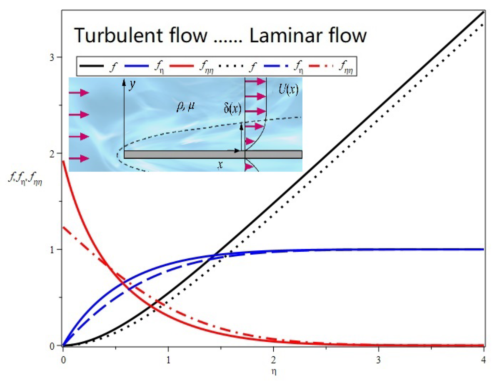

Table 1.
Prandtl magnitude order in boundary layer
| Variable | Magnitude order | |
|---|---|---|
| ≪ | ||
| ∼ | ||
| ∼ | ||
| ∼ | ||
| ∼ |
Table 2.
vs.
| 0 | 0.1 | 0.2 | 0.3 | 0.4 | 0.5 | 0.6 | 0.7 | 0.8 | 0.9 | 0.95 | 0.97 | |
|---|---|---|---|---|---|---|---|---|---|---|---|---|
| 1.401 | 1.466 | 1.535 | 1.611 | 1.692 | 1.799 | 1.873 | 1.923 | 1.944 |
Note: Laminar flow: , Turbulent flow: .
Disclaimer/Publisher’s Note: The statements, opinions and data contained in all publications are solely those of the individual author(s) and contributor(s) and not of MDPI and/or the editor(s). MDPI and/or the editor(s) disclaim responsibility for any injury to people or property resulting from any ideas, methods, instructions or products referred to in the content. |
© 2025 by the authors. Licensee MDPI, Basel, Switzerland. This article is an open access article distributed under the terms and conditions of the Creative Commons Attribution (CC BY) license (http://creativecommons.org/licenses/by/4.0/).
Copyright: This open access article is published under a Creative Commons CC BY 4.0 license, which permit the free download, distribution, and reuse, provided that the author and preprint are cited in any reuse.


