
Submitted:
07 March 2025
Posted:
10 March 2025
You are already at the latest version
Abstract
In the realm of fluid dynamics, turbulence inherently necessitates the interactions between fluid viscosity and velocity gradients. This study delves into the foundation of fluid motion equations, identifying the determination of the fluid's constitutive equation as the sole artificial element in their derivation. The paper posits that in turbulent flows, characterized by intense velocity gradients, the second-order terms associated with the deformation rate in the constitutive equation must be retained, rather than dismissed. This revelation yields an accurate constitutive equation for viscous fluids, enabling the derivation of fluid dynamics equations tailored for turbulent motion, devoid of adjustable parameters, and thus refining the Navier-Stokes equations. As a practical application, we present an extended version of Prandtl's boundary layer equation and provide a numerical solution for the wedge flow boundary layer. Determination formulation of the second-order viscosity coefficient is proposed and discussed.
Keywords:
Navier-Stokes equations
; turbulent flows
; constitutive equations
; velocity gradient
; boundary layers
1. Introduction
Turbulence is a term that swiftly conjures up a well-known adage: it stands as one of the most formidable challenges in physics and is often cited as one of the "unsolved problems in classical physics." The quest to unravel turbulence has consumed the brilliant careers of notable physicists and mathematicians, including Werner Heisenberg, Richard Feynman, and Andrei Kolmogorov, yet it remains unsolved. It is whimsically legacy that the esteemed physicist Horace Lamb intended to inquire about turbulence in the afterlife, should he meet the divine [1,2].
The quantitative quest to understand turbulence dates back to 1895 with Reynolds’ [3] pioneering efforts to analyze the Navier-Stokes equations for viscous fluids through the lens of average statistical methods, giving rise to the Reynolds averaged Navier-Stokes (RANS) equations. This endeavor has spanned over a century and a third, with every imaginable mathematical apparatus and computational resource brought to bear on the problem. Despite this, no seminal advance or breakthrough has emerged [4,5,6,7,8]. Since the formulation of the RANS equations, the demand of numerous engineering applications has led to the deployment of a spectrum of approximation techniques to close the RANS equation set. A multitude of models have been suggested to account for the elusive Reynolds stresses [9,10,11,12,13,14,15,16,17,18]. The question remains: can a universal closure theory for turbulence be crafted that accurately predicts turbulent motion across a range of scales? Regrettably, after 130 years of collective scientific endeavor, such a theory remains elusive. Instead, the plethora of models proposed to date are underpinned by non-rigorous assumptions, typically grounded in experimental observations, and each carries its own set of limitations [17,18,19].
Despite the significant strides made in direct numerical simulation (DNS) of turbulence, as documented in studies by Orszag [20], Rogallo et al.[21,22], Spalart [23], and Moin [24], and the recent advent of big data and artificial intelligence (AI) techniques in turbulence research, the intrinsic nature of turbulent flow remains an enigma. As we stand at the cusp of the AI era, gazing towards the horizon of discovery, we are compelled to pose a resounding question: What is the trajectory to the resolution of turbulence? Must we await the advent of quantum computing to unravel the enigmas through expansive numerical simulations? Across the span of 130 years of numerical simulation history, a pivotal truth endures: all simulation efforts are grounded in the Navier-Stokes equations, which are considered to encapsulate the entirety of turbulent phenomena, as evidenced by the work of [2,8,15,17,18,26]
Confronted with this legacy, we are at a crossroads with two distinct avenues of thought: one that advocates for a continued pursuit along the path defined by the Navier-Stokes equations, and another that suggests a return to the foundations, a reevaluation of the equations of fluid motion from their inception. This reflective approach challenges whether the Navier-Stokes equations should be further refined or enhanced to account for both turbulent and laminar flows without resorting to the Reynolds averaging methods, as proposed by Reynolds in 1895 [3].
In pursuit of clarity amidst the shadows, let us survey the historical landscape that gave rise to the equations governing fluid motion. Euler’s seminal contribution laid the groundwork for the mathematical depiction of fluid flow, envisioning it as a three-dimensional field of pressure and velocity that evolves through space. He conceptualized the flow as a continuum of infinitesimal fluid elements, deriving two interwoven nonlinear partial differential equations from the principles of mass conservation and Newton’s second law. While Euler’s equations mark a pivotal advance in theoretical fluid dynamics, their general solutions prove elusive. Notably, Euler’s framework omitted the frictional forces affecting fluid element’s viscosity-rendering his equations inadequate for real-world flow phenomena.
It took another century for the incorporation of frictional forces into Euler’s equations, culminating in the more intricate system we now recognize as the Navier-Stokes equations. Introduced independently by Navier in 1822 and Stokes in 1845, this system expands upon Euler’s with a set of nonlinear partial differential equations that account for the internal friction within the flow field. The Navier-Stokes equations, encapsulated in the momentum conservation equation and the incompressible mass conservation equation , where denotes the flow velocity field, p the pressure, t time, the mass density, and the kinematic viscosity, stand as the quintessential model for fluid flow description. Despite their preeminence, the quest for general analytical solutions to the Navier-Stokes equations persists, an endeavor that has eluded resolution to this day, as noted by [29,30,31].
In the pivotal year of 1895, Reynolds embarked on a groundbreaking investigation into turbulent flow by employing statistical averaging techniques. He deconstructed the fluid velocity into its mean component and its fluctuating component , such that the total velocity is given by the sum . Through the process of time-averaging the Navier-Stokes equations, he derived the Reynolds-Averaged Navier-Stokes (RANS) equations, formulated as , with the objective of capturing the mean values of key parameters in fluid dynamics. Despite this, the RANS equations are complicated by the inclusion of the fluctuating velocity correlation term , referred to as Reynolds stress, despite not truly being a stress [19]-rendering the equations intrinsically unclosed.
The prevalence of turbulence models grounded in the Reynolds-Averaged Navier-Stokes (RANS) equations is immediately apparent, each model striving to infer the connection between the turbulent viscosity coefficient and the mean velocity field through diverse lenses. Central to these efforts is the Boussinesq hypothesis, which posits , where k denotes the turbulent kinetic energy density. Essentially, the Boussinesq hypothesis conceptualizes as a stress-like quantity and, by emulating the linear constitutive relationship of Newtonian fluids, fabricates a potential linkage between and the mean flow velocities. The motivation behind the myriad models proposed for stems from a belief that turbulence originates from this term , a notion that is, in fact, a misapprehension.
Indeed, the term arises from the convective acceleration within the fluid motion, encapsulated by , and is an artifact of the Reynolds averaging procedure. Specifically, the Reynolds averaging of the fluid acceleration yields , where the mass conservation condition allows us to express the averaged fluid acceleration as . This indicates that the emergence of is independent of fluid viscosity; it merely represents the interaction of fluid velocity with its gradient. Moreover, the inviscid Euler equation, which omits the viscous term , also yields upon Reynolds averaging. As George has pointed out [18], is not a stress, but rather a transformed representation of the fluctuating contributions to the nonlinear acceleration terms. Since inviscid fluids are incapable of generating turbulent motion, it is clear that is not the root cause of turbulence.
The enigma of turbulence generation lies at the heart of fluid mechanics. While the precise prediction of turbulence remains an elusive goal, our understanding has crystallized around the conditions under which it does not arise: in the realm of inviscid fluid flows, turbulence is absent. The current conceptualization of turbulent flow can be summarized at a macroscopic level as follows: the interplay between fluid viscosity and velocity gradients is the principal catalyst for turbulence. Viscosity gives rise to vorticity in flows characterized by non-zero velocity gradients, precipitating fluid rotation. In response to mass conservation, the fluid must compensate for the mass that is displaced. Furthermore, the nonlinear nature of the convection term introduces a intricate pattern of motion. As the velocity gradient diminishes, the flow tends towards laminarity; conversely, when the velocity gradient intensifies, the flow transitions towards a turbulent state.
In the existing framework of the Navier-Stokes equations, a single term, , within the equation , encapsulates both the viscosity coefficient and the gradient of velocity , specifically its divergence . However, a limitation arises as the Reynolds averaging process yields , leaving the divergence with only the mean component , excluding the fluctuating parts. This suggests that the Navier-Stokes equations, as formulated with , , and , might not capture the full spectrum of viscous fluid dynamics and are, therefore, potentially incomplete, calling for an adjustment. Since is derived from the linear constitutive relation of viscous fluids in conjunction with the mass conservation condition , or , it is imperative to revisit the fluid’s constitutive relationship to ensure the inclusion of the comprehensive dynamics of fluid motion.
To derive the equations that govern turbulent flow, we must return to the foundational concepts of fluid mechanics by deriving the momentum conservation equation from a "first principles" approach. The concept of "first principles" dates back to ancient Greek philosophy, where Aristotle introduced it in his seminal work, "Metaphysics." According to Aristotle, first principles are the most elementary propositions or assumptions that are not derived from anything more fundamental; they serve as the bedrock for all knowledge and logical reasoning. This approach involves delving into the core of a subject, examining its most basic principles and assumptions, to forge new cognitive structures or solutions. Elon Musk has been a prominent advocate for this term, expressing his admiration for the "first principles" thinking method in interviews: "By applying first principles thinking, I distill the essence of matters and work up from the most fundamental truths..." He emphasizes the importance of this perspective over comparative thinking, which can lead to merely incremental advancements. First principles thinking, as Musk describes it, involves analyzing the world with a physicist’s lens, peeling back the layers of appearance to understand the intrinsic nature of things, and then constructing from this essence in a systematic manner. This is Musk’s interpretation of the "first principles thinking model" - a method of tracing the origins of concepts and reevaluating conventional approaches. The Navier-Stokes equations have stood as a cornerstone of fluid dynamics since their establishment in 1822. To achieve significant breakthroughs in our understanding, we must adopt a first principles mindset, beginning our inquiry from the ground up.
2. General Equations of Motion for an Incompressible Viscous Fluid
We know that before introducing the fluid constitutive relation, the mass conservation equation for incompressible fluids is , and the momentum conservation equation is: . The momentum conservation equation can also be rewritten in the form of tensor total quantity as follows:
where is body force density, is the stress tensor, are the components of the stress tensor, are the unit base vectors in the Cartesian coordinate system, and is the gradient operator and is right divergence of the stress tensor , whose computational rule is , in general . Equation 1 is the most general form of the momentum balance equation for a continuum and can be applied to describe the motion of any continuum.
To obtain a closed set of governing equations, we need to introduce the fluid’s constitutive relation, which is the relationship between the stress tensor and the rate-of-strain tensor , namely , where is the rate-of-strain tensor, and its components are .
It is important to recognize that the introduction of a fluid’s constitutive relation involves a degree of human interpretation in comprehending the physical attributes of the fluid. This interpretive aspect is perhaps the most subjective element in formulating the equations of fluid motion. From Navier to Stokes, the prevailing assumption has been that fluids are isotropic and incompressible, leading to a proposed linear relationship between the stress tensor and the rate-of-strain tensor as expressed by , where denotes the viscosity coefficient. This constitutive relation was conceived in a time bereft of tensor theory and has since been universally embraced by the scientific literature. In the context of modern science, with our understanding of tensors, it is incumbent upon us to question whether the relationship between the stress tensor and the strain rate tensor can be articulated more rationally, and if so, to determine the appropriate form for this new expression.
Assuming the fluid’s physical properties are isotropic, since both the stress tensor and the rate-of-strain tensor are second-order tensors, according to the tensor representation theory [33,34,35,36], the most general expression for the constitutive relation of an incompressible fluid can always be written as follows:
where ; the term is not referred to by name in the literature; in this text, it is termed the second-order viscosity coefficient with dimensions dim .
To determine the entropy inequality for the given Cauchy stress tensor , we start from the Clausius-Duhem inequality, which enforces the second law of thermodynamics. For simplicity, we consider isothermal conditions and focus on the mechanical dissipation part of the entropy inequality. The Clausius-Duhem inequality [33,34,35,36] under isothermal conditions reduces to: , where is the rate of deformation tensor (symmetric part of the velocity gradient), is the density, and is the Helmholtz free energy, in which is double dot product of two tensor and with computational rule: .
For a fluid where the stress tensor is given, we substitute into the inequality . The stress tensor is: . Substituting this into the dissipation term . Since , and , noting the symmetric tensor , leads to . Thus, the dissipation term becomes: . For an incompressible fluid, , simplifying the dissipation term to: .
The entropy inequality requires this term to be non-negative for all possible . Therefore, the entropy inequality for the given stress tensor is: , which satisfy the second law of thermodynamics for all possible flow motion [33,34,35,36,33].
The fluid viscosity leads to the dissipation of energy, which is ultimately converted into heat. The energy dissipation per unit time for an incompressible viscous fluid is given by
where represents the volume configuration of the fluid control body.
In the annals of fluid mechanics, from the works of Navier and Stokes to contemporary research, fluids have consistently been treated as Newtonian, employing the linear constitutive relation , while the second-order term has been omitted. The exclusion of the term can be attributed to two primary factors. Firstly, during the era of Newton, Navier, and Stokes, nonlinear effects were not detectable, and the necessary tools for tensor analysis, including tensor representation theory and the Cayley-Hamilton theorem[37], were not yet developed; indeed, the Cayley-Hamilton theorem was published after the formulation of the Navier-Stokes equations. Secondly, even if the expression Equation 2 were to be derived, it was generally assumed that the second-order term was sufficiently insignificant to be disregarded. That is to say, the second-order constitutive relation, , is the correct and complete result, whereas its first-order constitutive relation is actually an approximation. This was not understood in the era before the development of tensor representation theory.
This study contends that the omission of the second-order term in the formulation of fluid mechanics equations is a critical oversight. Given that the spatial variation of velocity, such as the gradient near a wall, can be extremely pronounced, neither the first nor the second power of the velocity gradient should be dismissed. This resonates with the scenario encountered in the boundary layer theory. Prandtl [38] emphasized, upon introducing the boundary layer concept, that the Reynolds number in the term must not be ignored, regardless of how high the value of (or how low ) may be, because the velocity gradient is sufficiently steep to render the entire term significant.
Bringing Equation 2 into Equation 1 allows us to derive the fluid motion equation that considers second-order viscosity:
wherein, the kinematic viscosity is , and the kinematic second-order viscosity is with dimensions dim . Equation 4 represents the most general equation of motion for viscous fluids. The viscosity coefficients are generally functions of pressure p and temperature T, and they cannot be factored out of the gradient operator.
In most cases, the viscosity coefficients do not vary significantly within the fluid and can be considered as constants. Under the incompressible condition , Equation 4 can be simplified to:
where the Laplacian . In this way, we have improved the Navier-Stokes equation to Equation 5, which is the most general equation of motion for incompressible viscous fluids. The term includes the nonlinear combination of the fluid’s second-order viscosity and velocity gradients, which is the main cause of complex flow phenomena. Since Equation 5 already includes higher-order terms of the velocity gradient, it can be directly used to simulate turbulence without the need to employ Reynolds’ statistical averaging method, which is the statistical decomposition of the fluid velocity.
Equation 5 can be written in component form as follows:
It should be particularly noted that for problems with specific characteristic length and characteristic velocity , the dimensionless process of Equation 5 not only yields the Reynolds number , but Equation 5 also generates a new dimensionless parameter, denoted as . The parameter arises due to the consideration of second-order viscosity. For a fluid with a given , this parameter is independent of the characteristic velocity and only related to the characteristic length , or in other words, for flow problems of a given length scale, the parameter affects the fluid motion for all characteristic velocity scale. Therefore, it is necessary to retain the second-order viscosity coefficient.
The tensorial Equation 6 can be further expanded in conventional form, in the Cartesian rectangular coordinate system, denoting , , , , , the three-dimensional fluid momentum equation can be read as follows:
where , and . The difference from the Navier-Stokes equations can be seen from the above equations, namely, each equation includes higher-order terms of the velocity gradient.
After using the continuity equation the two-dimensional momentum equation is expressed as follows:
For the two dimensional flow, we have and . Noice continuity condition , results to , thus, we have in conventional forms and . The entropy inequality can be expressed as to:
For heat conduction problems, it is assumed that there is a heat flux density , where T is the temperature and is the thermal conductivity. The general equation of heat transfer is given by
where s is the entropy density per mass [7].
3. Boundary Layer Theory and Application to Wedge Flow
In 1904, at the third International Congress of Mathematicians, Ludwig Prandtl [38] unveiled the notion of the boundary layer, proposing that the effects of frictional forces are primarily restricted to a slender layer adjacent to an object’s surface. Inside this boundary layer, both the velocity gradient and the shear stress are substantial, generating a frictional resistance that must be accounted for. The equations governing the boundary layer are notably less complex than the full Navier-Stokes equations and can be addressed numerically[39]. Notably, Prandtl identified that the flow within the boundary layer can exhibit turbulence[40,41], and in 1925, he introduced the concept of the mixing length to quantify the turbulent viscosity[42]. This concept was instrumental in formulating the logarithmic law for the wall in turbulent boundary layers and represented a pivotal effort to close the Reynolds-Averaged Navier-Stokes (RANS) equations.
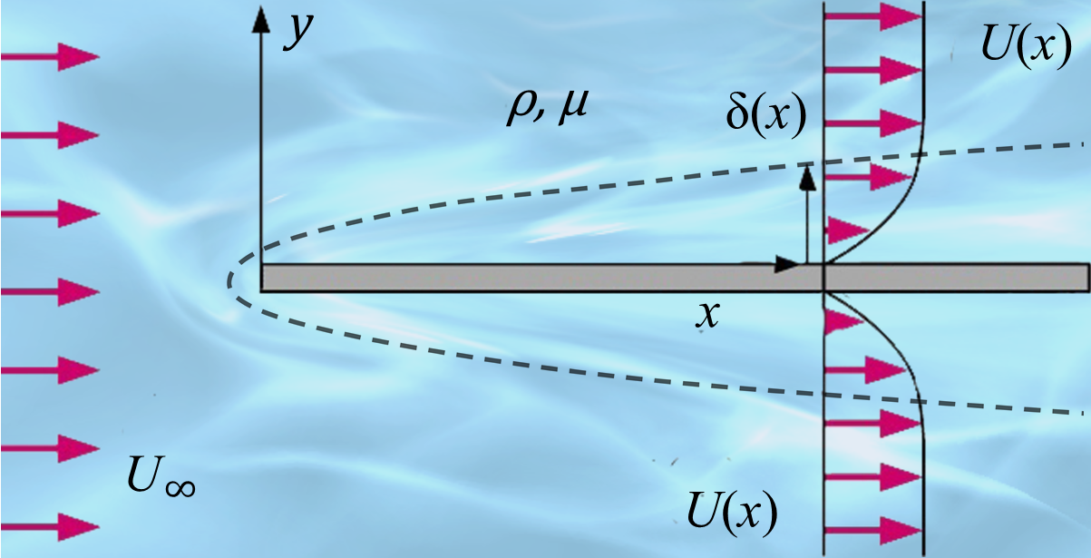
In 1908, Prandtl’s student Blasius[39] studied the problem of steady flat-plate boundary layers. A thin flat plate is immersed at zero incidence in a uniform stream with speed and is assumed not to be affected by the presence of the plate as shown in Figure 1, except in the boundary layer. The fluid is supposed unlimited in extent, and the origin of coordinates is taken at the leading edge, with x measured downstream along the plate and y perpendicular to it. Blasius[39] performed a similarity transformation on Prandtl’s equations and and successfully obtained a numerical solution for the problem. In 2024, Sun[43] studied unsteady laminar boundary layers and applied a similarity transformation to the equations and , successfully obtaining an exact solution for the unsteady flat-plate laminar boundary layer. This solution is primarily expressed in terms of Kummer functions, and other flow problems were also investigated.
Based on the Prandtl’s magnitude analysis and approximations as shown in Table 1, we can obtain the boundary layer equations as follows:
The underlined segment represents the manifestation of the second-order theory proposed in this paper, which is where it differs from Prandtl’s boundary layer equations. The exact solution of partial differential equation systems in Equations 14 and 15 can be easily solved by using Maple, the solutions of velocity components and are mainly expressed in terms of Lambert function[45]: LambertW=, which satisfies: . Although we can obtain the solution, it is regrettable that the integral involving the Lambert function cannot be calculated explicitly at the moment, making this solution less applicable. Let us try other methods below.
Introducing a stream function and express the velocity components as follows: , the mass conservation Equation is satisfied, and the momentum conservation Equation 14 becomes
and corresponding boundary conditions.
Applying Sun’s similarity transformations [43]: . Denoting and , and noting the and , and by the chain rule for derivatives, we can obtain some useful relations as follows: . Thus the velocity components become
Substituting Equation 17 and Equation into Equation 16, we have a single partial differential equation as follows
where the coefficients are , , and and their relation .
If the coefficient , and were constants, then we have: , where the exponent . It is clear, for arbitrary , that the Equation 19 explicitly contains the coordinate x, which conn’t be solved easily for arbitrary exponent m.
In the case of wedge flow with velocity field: , so that , then and , and leads to a constant boundary thickness . If we set , we have , and the Equation 19 becomes
and boundary conditions: , and , where is a constant for given a problem. Equation 20 has get rid of coordinate x, can be solved numerically.
For its corresponding steady problem, the function f is only a function of , the Equation 20 can be simplified into:
and boundary conditions: and . Equation 21 not only facilitates solving the equation but also allows us to express the obtained results as a single profile in terms of the similar variable .
Although we do not yet have specific data for , we can still assume for the laminar boundary layer and for the turbulent boundary layer. Using the program provided above, it is easy to calculate the corresponding for both laminar and turbulent flow. The specific results are shown in Figure 2. From the profile of , it can be seen that the velocity profile in turbulent flow is blunter than that in laminar flow; from the profile of , it can be observed that the friction in turbulent flow is much greater than that in laminar flow.
To demonstrate the difference in frictional resistance between turbulent and laminar flow, let’s calculate the shear stress . Considering the order of magnitude approximation estimates of the Prandtl boundary layer theory in Table 1, the shear stress can be approximated as: . Therefore, the local wall shear stress is given by :
This expression reveals that the resistance of the flow with is much greater than that of the flow with . Table 2 lists the different corresponding to different ; the larger the , the greater the .
Up to this point, there is still one issue that has not been resolved, which is to verify the entropy inequality. If we apply Equation 12 to the wedge flow, noting the relationships , the entropy inequality can be expressed as follows:
which holds if .
4. Steady Incompressible Flow in an Inclined Pipe and Determination of the Second Viscosity
After establishing new equations for the incompressible fluids, one remaining question is how to determine the second-order viscosity coefficient . Below, let’s demonstrate through an example that, when the dynamic viscosity coefficient of the fluid is known, the second-order viscosity coefficient can be obtained using a simple experiment.
Consider steady incompressible flow in an infinitely long round pipe with a radius inclined at an angle (Figure 3). The fluid flows down the pipe due to gravity, meaning no applied pressure gradient is present in the fluid.
We use the semi-inverse method, which involves first determining the general form of the flow velocity based on the problem’s conditions, then substituting this into various expressions to see under what boundary conditions the initially assumed flow velocity holds. Due to the pipe’s axial symmetry, we can assume the flow is also axisymmetric, and thus the velocity field can be expressed as a function of radius r only, , , and . The no-slip condition at the wall is , and there is pressure balance at the two ends of the pipe: and .
Using the conversion relationships between Cartesian and polar coordinates, , , , and substituting and , into the strain-rate tensor , we obtain . Using the differential relations , , this constitutive relation can be expressed in matrix form as follows:
For steady flow, and , , the continuity condition is automatically satisfied. The momentum equations are as follows:
Using the first and second expressions of Equation 25 and noting the chain rule of calculus, we get , since the right-hand side does not depend on z, the left-hand side must be a constant c (which is actually the pressure gradient along the z-direction), thus , where is an integration function. Substituting this into Equation 25 gives the third expression, leading to the equation , and considering the boundary conditions , , the solution can be written as
Bringing back into , we get , where is an integration function. Thus, the pressure is . Substituting this into , we obtain , and after integrating with Equation 26, we get , where d is an integration function. Therefore, the pressure can be expressed as
The Cauchy stress can then be further expressed as
Now, apply the boundary conditions at and to determine the undetermined constants c and d. On the cross-section at , the shear stresses are and , and the normal stress is . Similarly, on the cross-section at , the shear stresses are and , and the normal stress is . Applying these conditions to p and yields the boundary conditions: , , , , , . If , then it must be the case that , which corresponds to the situation with no pressure gradient. Therefore, the boundary stress conditions are as follows: , and , as well as , and . This means that, in order to obtain the velocity form , and assumed in advance by the semi-inverse method, the above pressure boundary conditions must be provided, with the resultant force and resultant bending moment being zero, such as the force over its area of application . If we set the pressure at to be equal to , i.e., , and considering there is no pressure gradient , we can determine , thus obtaining the following expression for pressure:
Since this expression includes the dynamic viscosity coefficient and the second-order viscosity coefficient , and given that is known, this expression can guide experiments to determine the second-order viscosity coefficient . For simplicity, if we place the circular pipe vertically (as in Figure 3), at this point , the pressure expression becomes simpler: . If we can measure the pressure at the axis of the circular pipe , we can obtain the following expression to predict the second-order viscosity coefficient :
With the above relation, we can determine the second-order viscosity by the fluid flowing down the pipe due to gravity alone. Especially from the structure of this expression in Equation 30, it can be seen that for a fluid with known , its corresponding second-order viscosity coefficient is directly proportional to the pressure difference between the pipe wall and its center on a unit area.
5. Discussions and Conclusions
In the light of the theoretical developments and practical applications presented herein, the quadratic term emerges as a pivotal element in the depiction of turbulent flow dynamics. It is arguable that the Navier-Stokes equations, devoid of the term, are fundamentally tailored to laminar flow phenomena and are insufficient for capturing the intricacies of turbulent motion. The pronounced velocity gradients inherent in turbulence necessitate the retention of the term; its omission would preclude an accurate representation of turbulent behavior in the derived equations.
While the focus of this work is on the turbulence regime, the equations Equation 5 and Equation 6 that have been formulated are, in fact, universally applicable to the motion of viscous fluids. The derivation of these equations is underpinned by logical consistency at each stage, eschewing any arbitrary approximations. These equations hold potential for a wide range of incompressible viscous fluid flows, including aerodynamic gas dynamics and the acoustic emissions from turbulent processes. The same conceptual framework employed for Equation 2 can be extended to establish motion equations for compressible viscous fluids as shown in the Appendix.
Data Availability Statement
The data supporting the findings of this study are available from the corresponding author upon reasonable request.
Acknowledgments
Following the online publication of my paper [43] on August 20, 2024, I reached out to Professor Shing-Tung Yau, a distinguished Fields Medalist, via WeChat, seeking his insights and feedback. Professor Yau promptly responded and extended an invitation for me to present a lecture. On September 11, 2024, I delivered a talk based on my paper [43] at the Tsinghua University Yau Mathematical Science Center (YMSC). The very next morning, on September 12, 2024, Professor Yau messaged me on WeChat, proposing that I organize a seminar series in mechanics at the YMSC. In response, I launched two seminar series: "Dimensional Analysis and Scaling Laws" and "Tensor Analysis and Applications." After the conclusion of the "Dimensional Analysis and Scaling Laws" series on November 8, 2024, Professor Yau gathered with the participants for feedback and a group photograph. During this session, he referred to the celebrated mathematician C.C. Lin and mentioned Lin’s assertion of having solved certain turbulence problems, seeking my perspective on the matter. I acknowledged the complexity of turbulence and the unresolved issues within the field. Professor Yau’s inquiry sparked deep reflection on my part. I reflected on my challenging journey in turbulence research and concluded that adhering to the prevailing methodologies would not suffice to crack the turbulence puzzle. As the adage goes, "The issue is not the inability to act, but the failure to imagine." To tackle turbulence, innovative thinking is imperative, and the conventional Navier-Stokes equations require modification. Consequently, I re-examined the equations of fluid motion and identified that the determination of the fluid’s constitutive equation is the sole aspect involving human judgment. Utilizing my tensor analysis expertise, I quickly perceived the inadequacy of the linear constitutive equation for Newtonian fluids and its need for revision at a rational level. This realization paved the way for the derivation of the fluid motion equation presented in this article. To clarify the origins of this innovative approach, I have documented it here as a memorandum for this research, and I also wish to express my heartfelt gratitude to Professor Yau for his inquisitiveness, which catalyzed my reevaluation of the turbulence problem [44].
Conflicts of Interest
The authors declare that there are no competing financial interests.
Appendix 1 Introduction
The approach to modifying the fluid’s constitutive relations here is universal and can be extended to any other fluid mechanics problems, such as compressible fluids, magnetohydrodynamics, mass and heat transfer in fluids, aerodynamics and gas dynamics, etc. Below, only the equations for two scenarios are listed.
Appendix 2 Motion Equations for Compressible Viscous Fluids
Continuity equation:
Momentum equations:
Energy equation:
Constitutive equation:
where is stress-temperature modulus, and strain rate tensor: .
Appendix 3 Motion Equations for Compressible Mixture Viscous Fluids (Diffusion)
Continuity equation:
where c is concentration of mixture.
Momentum equations:
Energy equation:
where is heat flux, is chemical potential of the mixture, Constitutive equation:
where is stress-temperature modulus, and strain rate tensor: .
References
- G. Falkovich and K. Sreenivasan, Lessons from hydrodynamic turbulence. Physics Today 43, 2006.
- P. A. Davidson, Y. Kaneda, K. Moffatt, Katepalli R. Sreenivasan, A Voyage Through Turbulence, Cambridge University Press, Cambridge (2011).
- O. Reynolds, On the dynamical theory of incompressible viscous fluids and the determination of the criterion. Phil.l Trans. Royal Soc. London. 186, 123-164 (1895). [CrossRef]
- L. F. Richardson, Weather Prediction by Numerical Process (Cambridge University Press, Cambridge, England, 1922). [CrossRef]
- H. Tennekes and J.L. Lumley, A First Course of Turbulence. (The MIT Press, Cambridge, 1972).
- H. Schlichting, Boundary Layer Theory, McGraw-Hills, 1960 translated by J. Kestin.
- L.D. Landau and E. M. Lifshitz, Fluid Mechanics, (Butterworth-Heinemann, 1987).
- U. Frisch, Turbulence: The Legacy of AN Kolmogorov (Cambridge University Press, Cambridge, England, 1995).
- P. Bradshaw and W. A. Woods, An Introduction to Turbulence and its Measurement (Pergamon, New York, 1971).
- T. Cebeci, Analysis of Turbulent Boundary Layers (Academic Press, New York, 1974).
- A.S. Monin and A.M. Yaglom, Statistical Fluid Mechanics: Mechanics of Turbulence (MIT Press, Cambridge, MA, 1975).
- A.A. Townsend, The Structure of Turbulent Flow (Cambridge Univ. Press, New York, 1976).
- O.A. Oleinik and V.N. Samokhin, Mathematical Models in Boundary Layer Theory (CRC Press, London, 1999).
- P. S. Bernard and J. M. Wallace, Turbulent Flow Analysis, Measurement, and Prediction (John Wiley & Sons, New Jersey, 2002).
- F. M. White, Viscous Fluid Flow (McGraw-Hill, New York, 2006).
- B. Birnir, The Kolmogorov-Obukhov Theory of Turbulence (Springer, New York, 2013).
- D. C. Wilcox, Turbulence modeling for CFD (DCW Industries, Inc. California, 1993).
- P.A. Davidson, Turbulence (Oxford University Press, Oxford, 2004).
- W. K. George, Lecture in Turbulence for the 21st Century. Free online book. http://turbulence-online.com/.
- S.A. Orszag and G.S. Patterson, Numerical simulation of three-dimensional homogeneous isotropic turbulence. Phys. Rev. Lett. 28:76-79(1972).
- R.S. Rogallo, Numerical experiments in homogeneous turbulence. NASA TM-81315 (1981).
- R.S. Rogallo and P. Moin, Numerical simulation of turbulent flows. Annu. Rev. Fluid Mech. 16:99-137(1984).
- P. R. Spalart, Direct simulation of a turbulent boundary layer up to Rθ=1410, J. Fluid Mech. 187:61-98(1988).
- P. Moin and K. Mahesh, Direct numerical simulation: A tool in turbulence research. Annu. Rev. Fluid Mech. 30:539-78(1998).
- S. B. Pope, Turbulent Flows (Cambridge University Press, 2000).
- P. Y. Chou, On velocity correlations and the solutions of the equations of turbulent fluctuation. Q Appl Math 1945; 111(1):38-54.
- C. Navier, Mémoire sur les Lois du Mouvement des Fluides. Mém.del’Acad. des Sciences. 1822;vi.389.
- G.G. Stokes, On the theories of the internal friction of fluids in motion and of the equilibrium and motion of elastic solids. Trans. Cambridge Philos. Soc. 8,287-319(1845).
- O. Ladyzhenskaya, The Mathematical Theory of Viscous Incompressible Flows (2nd edition) (Gordon and Breach, New York, 1969).
- J.D. Anderson Jr, Ludwig Prandtl’s boundary layer, Physics Today, 58(12)42-48(2005).
- C.L. Fefferman, Existence and smoothness of the Navier-Stokes equation, The millennium prize problems, Clay Math. Institute, pp.57-67(2006).
- The First Principles Method Explained by Elon Musk, Dec 4, 2013 Interview by Kevin Rose, https://www.youtube.com/watch?v=NV3sBlRgzTI.
- R. S. Rivlin and J. L. Ericksen, Stress-Deformation Relations for Isotropic Materials. J. Rat. Mech. Anal. 4, 323-425(1955).
- R. S. Rivlin, Further remarks on the stress-deformation relations for isotropic materials. J. Rat. Mech. Anal. 4,5:681-702 (1955).
- C. Truesdell and W. Noll,The Non-Linear Field Theories of Mechanics. Handbuch der Physik, Editors: S.Flugge, Vol3, Springer-Verlag, Berlin(1969).
- C. Truesdell, A First Course in Rational Continuum Mechanics (Academic Press, New York, 1977).
- A. Cayley, A Memoir on the Theory of Matrices. Philos. Trans. 148.(1858).
- L. Prandtl, On fluid motions with very small friction (in German). Third International Mathematical Congress, Heidelberg (1904).
- H. Blasius, Grenzschichten in Fljssigkeiten mit kleiner Reibung. Z. Math. Phys. 56:1-37(1908).
- L. Prandtl, Bemerkungen über die entstehung der turbulenz, Z. Angew. Math. Mech. 1:431-436(1921).
- Th. von Kármán, Über leminere und turbulence Reibung (On Laminer and Turbulent Friction), Z. Angew. Math. Mech. 1:223(1921).
- L. Prandtl, Bericht über Untersuchungen zur ausgebildeten Turbulenz, Z. Angew. Math. Mech. 5,(2):136-139(1925).
- Bo Hua Sun, Similarity solutions of a class of unsteady laminar boundary layer, Phys. Fluids, 36, 083616 (2024). [CrossRef]
- B. H. Sun, Thirty years of turbulence study in China. Appl. Math. Mech, 2019;40(2):193-214. [CrossRef]
- R.M. Corless, G.H. Gonnet, D.E.G. Hare, D.J. Jeffrey, and D.E. Knuth, On the Lambert W Function. Advances in Computational Mathematics, Vol. 5, (1996): 329-359.
Figure 1.
A thin flat plate is immersed at zero incidence in an uniform stream flows with velocity and body force density .
Figure 1.
A thin flat plate is immersed at zero incidence in an uniform stream flows with velocity and body force density .
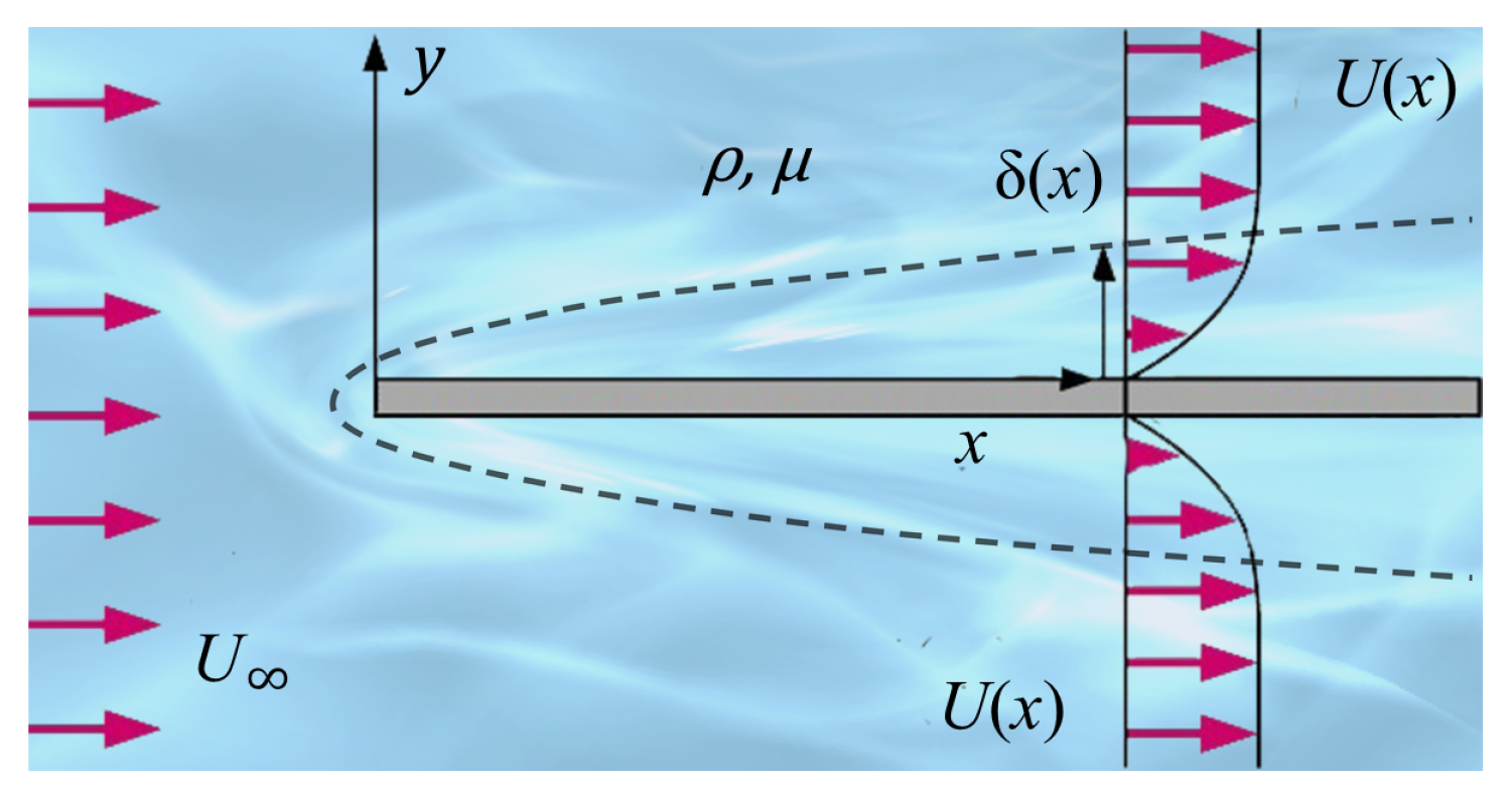
Figure 2.
Function and its derivatives and for parameter and
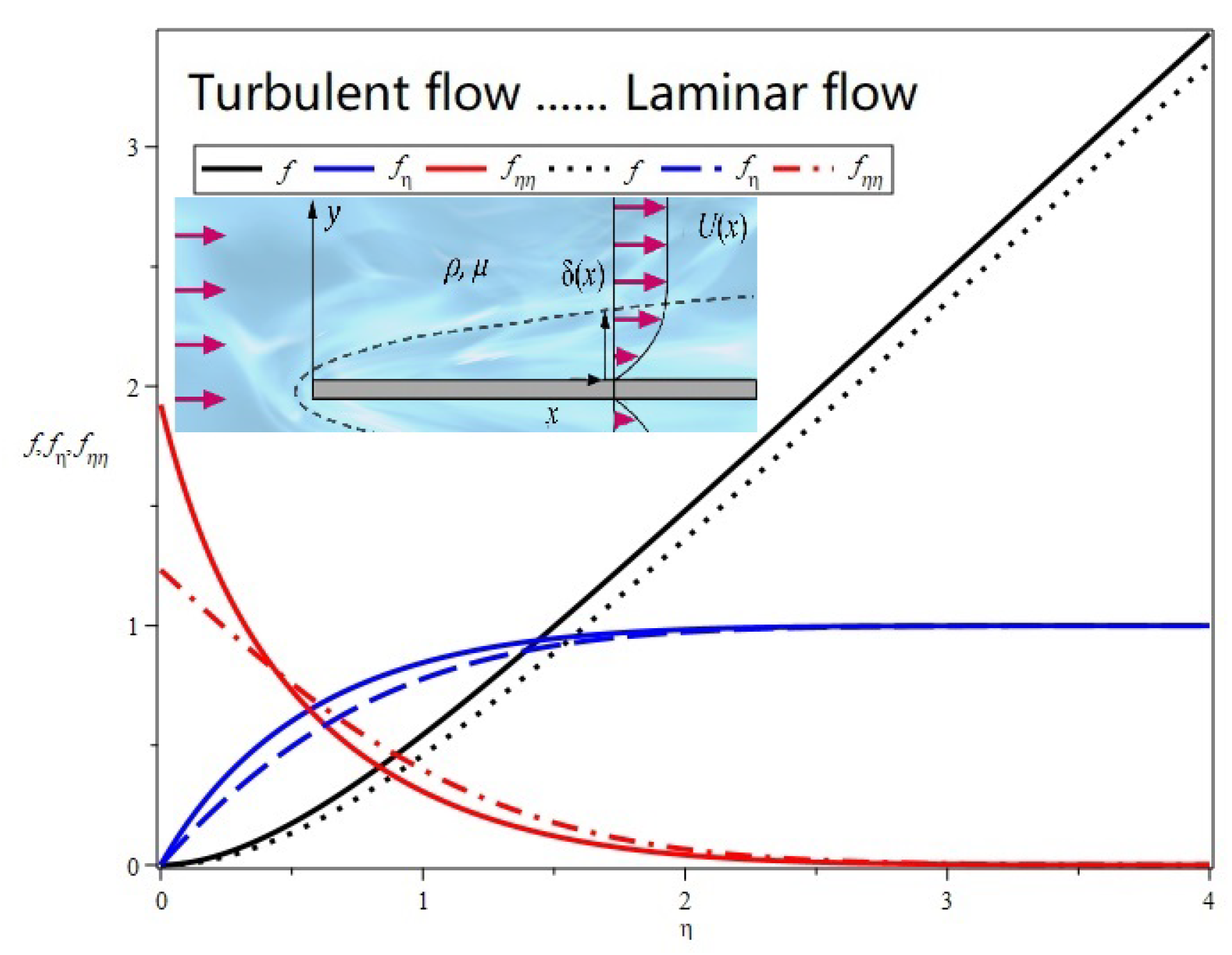
Figure 3.
Steady incompressible flow in an infinitely long round pipe of diameter D or radius : The left figure shows the pipe inclined at an angle , while the right figure is perpendicular to the ground with .
Figure 3.
Steady incompressible flow in an infinitely long round pipe of diameter D or radius : The left figure shows the pipe inclined at an angle , while the right figure is perpendicular to the ground with .
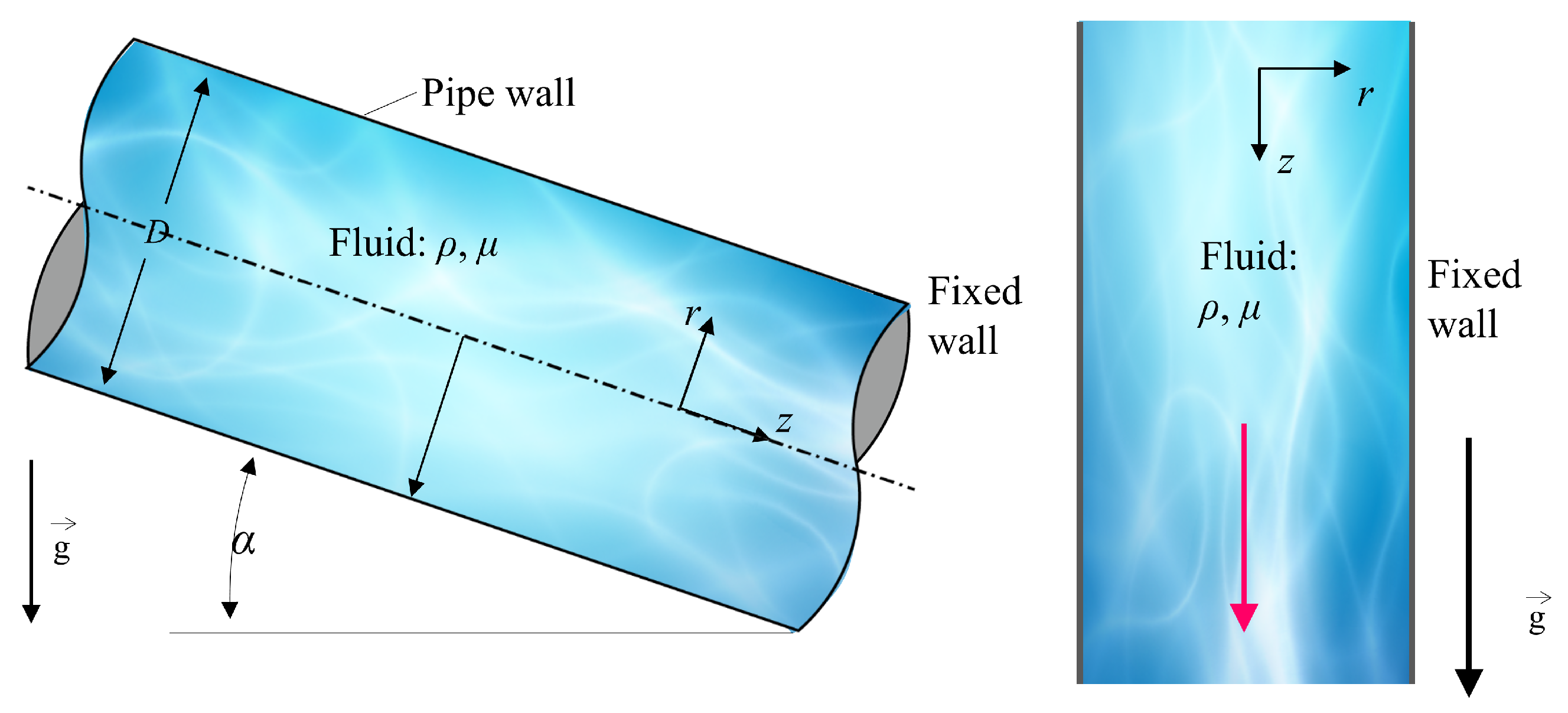

Table 1.
Prandtl magnitude order in boundary layer
| Variable | Magnitude order | |
|---|---|---|
| ≪ | ||
| ∼ | ||
| ∼ | ||
| ∼ | ||
| ∼ |
Table 2.
vs.
| 0 | 0.1 | 0.2 | 0.3 | 0.4 | 0.5 | 0.6 | 0.7 | 0.8 | 0.9 | 0.95 | 0.97 | |
|---|---|---|---|---|---|---|---|---|---|---|---|---|
| 1.401 | 1.466 | 1.535 | 1.611 | 1.692 | 1.799 | 1.873 | 1.923 | 1.944 |
Note: Laminar flow: , Turbulent flow: .
Disclaimer/Publisher’s Note: The statements, opinions and data contained in all publications are solely those of the individual author(s) and contributor(s) and not of MDPI and/or the editor(s). MDPI and/or the editor(s) disclaim responsibility for any injury to people or property resulting from any ideas, methods, instructions or products referred to in the content. |
© 2025 by the authors. Licensee MDPI, Basel, Switzerland. This article is an open access article distributed under the terms and conditions of the Creative Commons Attribution (CC BY) license (http://creativecommons.org/licenses/by/4.0/).
Copyright: This open access article is published under a Creative Commons CC BY 4.0 license, which permit the free download, distribution, and reuse, provided that the author and preprint are cited in any reuse.


