1. Introduction
The Discrete Fourier Transform (DFT) is a cornerstone of modern signal processing, enabling the transition between time-domain and frequency-domain representations of discrete signals. While the DFT is computationally intensive for large data sets, the development of Fast Fourier Transform (FFT) algorithms has revolutionized this field by significantly reducing computational complexity. Among the various FFT algorithms [
1], Radix-2, Radix-4, and Bluestein [
2] stand out for their unique advantages and applicability to different scenarios [
3].
This paper investigates the computational complexity of these three prominent FFT algorithms, which have been implemented and analyzed using MATLAB [
4]. Radix-2, known for its simplicity and efficiency for power-of-two data lengths, remains a widely adopted algorithm in many practical applications [
3]. On the other hand, Radix-4 enhances this efficiency by processing four data points at a time, reducing the number of stages and multiplicative operations. However, both algorithms are constrained by their dependence on specific sequence lengths.
The Bluestein algorithm, often referred to as the chirp-z transform method, addresses this limitation by enabling FFT computations for arbitrary sequence lengths, including prime numbers. By reformulating the DFT as a convolution problem, the Bluestein algorithm leverages FFTs to compute convolutions efficiently. While this approach introduces additional computational overhead, it eliminates the need for zero-padding, which can distort frequency-domain results in certain applications [
5].
To minimize computational complexity and assess the practical performance of these algorithms, MATLAB implementations were developed with optimization strategies to reduce the number of multiplications during runtime. These implementations facilitated a comparative analysis of the three algorithms, focusing on their multiplication and addition requirements across various data lengths.
This study aims to provide a comprehensive understanding of the trade-offs involved in selecting an FFT algorithm for specific applications. By evaluating the strengths and limitations of Radix-2, Radix-4, and Bluestein algorithms [
2], this research offers valuable insights into their suitability for diverse signal processing tasks. Additionally, the findings contribute to the ongoing development and optimization of FFT algorithms, ensuring their continued relevance in addressing the computational demands of modern signal processing applications.
2. Complexity of Radix-2 DIT/DIF Algorithm
A MATLAB program has been written and is in
Appendix 1, to compute the FFT of a set of discrete data:
where
and
n is an integer. A modification of the supplied Radix-2 program was made in order to reduce the number of multiplications involved and is highlighted in the attached Radix-2 program [
3,
6].
The final loop in the program made use of the property
, which allowed the number of multiplications in the final loop to be halved. The program uses a recursive procedure which calls up the FFT of the odd and even set of data points [
7].
In the special case when
, there are no multiplications to evaluate and only 2 additions. In the general case when
, the recursive procedure calls up the Fourier transform of two sets of data, each of length
. The final loop in the procedure contains
multiplications and
N additions. Using
,
, let
represent the number of computed multiplications and
represent the number of computed additions. It can be deduced that
and
satisfy the difference equations:
The solutions to these difference equations can be obtained by taking a
z-transform of the equation. It can be shown that the formulas for
and
[
7,
8] are given by:
The values for
and
have been tabulated as shown in the
Table 1 below:
This data is consistent with Cooley and Tukey algorithm [
1] formula
for large values of
N. The above results were programmed with MATLAB and are listed in
Appendix 1
3. Complexity of Radix-4 DIT/DIF Algorithm
A MATLAB program has been written and is in
Appendix 2, to compute the FFT of a set of discrete data:
where
and
n is an integer.
The program uses a recursive call of a function that computes the FFT of the odd and even data points. The original program was modified to reduce the loop length by a factor of 4 by making use of the property
. Hence, the number of multiplications in the loop was halved [
3].
In the special case when , there are no multiplications to evaluate and only 8 additions. In the general case when , let represent the number of computed multiplications in the program.
The program has 4 function calls of the FFT of data which is half the original length and therefore contains
multiplications. The for loop in the algorithm contains one multiplication which is repeated
times (i.e.,
times) [
5,
9]. Hence, the number of multiplications in the program can be computed from the sequence:
The solution to this difference equation can be shown to be given by [
10,
11]:
The number of additions in the program can be computed from the sequence:
The solution to this difference equation can be shown to be given by:
This sequence is tabulated for various values of
n and
N as shown in
Table 2 below:
Compared to Radix-2, the Radix-4 algorithm, for large
N, has reduced the number of multiplications by
, but the number of additions has remained unchanged [
1,
3].
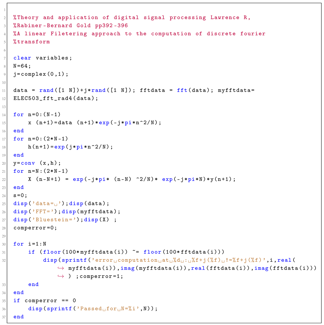
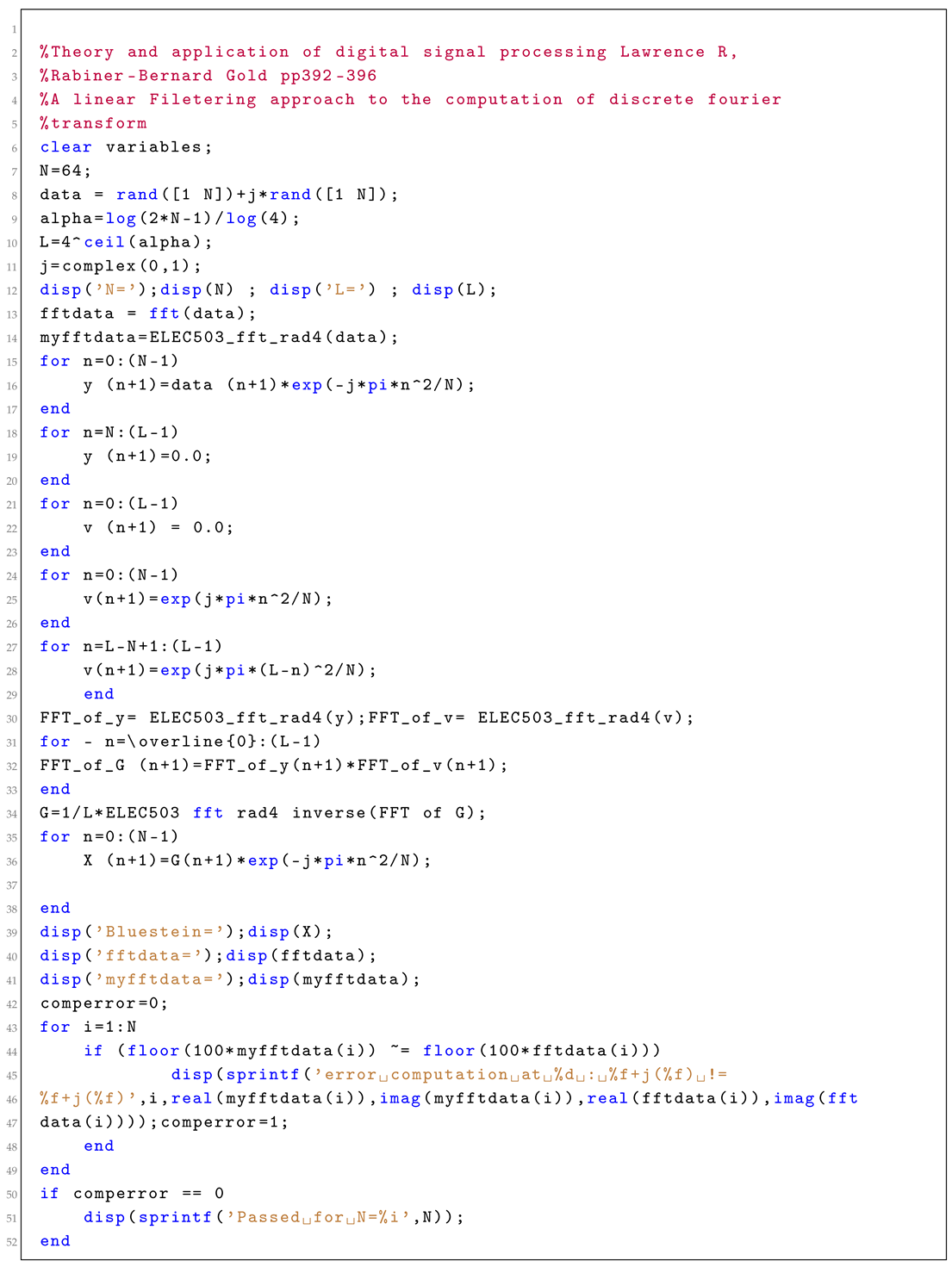
4. Complexity of Bluestein
The Bluestein algorithm [
2] is a digital filtering approach to determine the DFT of a set of data and is valid for any value of
N [
7,
8].
Consider an input sequence , , which is input to a digital filter with an impulse response
The output of the filter in the range
can be shown to be given by:
By substituting
into (9), the output of the filter can be expressed in the form:
This equation implies that
is the weighted output of the
N point DFT of the sequence
. This result suggests that the DFT of a sequence can be obtained by first pre-multiplying the input sequence by the factor of
and inputting this sequence to a digital filter [
10,
11,
12]. The output sequence can be obtained multiplying the filter output by a factor of
. This is called Bluestein’s algorithm [
2]. It should be noted that the filter output can be determined from the filter input by using a convolution of the impulse filter response and the input data [
13]. A MATLAB program has been written to determine the DFT of a random set of data which uses the built-in MATLAB convolution function [
7]. However, the complexity of the built-in MATLAB convolution function is not known. Therefore, a MATLAB program was written to evaluate the convolution using the result that the convolution of a function can be determined from the inverse transform of the transform products of the impulse response and the input data [
6].
The convolution calculation in our MATLAB program requires three calculations of the FFT transform of a signal, which is of length
[
5,
9]. However, we need not include the FFT transform of the impulse response in our complexity calculation, since this can be precalculated and is independent of the data [
6].
As seen in the modified Bluestein MATLAB program, the number of multiplications can be summarized as follows:
Bluestein Multiplications:
Since the FFT calculations in the Bluestein Algorithm used the Radix-4 algorithm [
14,
15], then the total number of multiplications computed,
, is given by the formula:
For large
N, this formula tends to
. This is an increase of
over the Radix-2 calculation [
16].
In the case of the addition complexity of the Bluestein algorithm in our program, this count is equal to the count of 2 FFT’s of length
, using the Radix-4 algorithm [
5].
For large
N, this value is four times that of the Radix-2 calculation.
It should be noted that the Bluestein algorithm is less efficient than the Radix-2 and Radix-4 algorithms [
17], but has the advantage that the value of
N does not need to be a power of 2 [
1,
9]. The above results were programmed with MATLAB and are listed in
Appendix 2.
6. Discussion and Conclusion
The computational complexity analysis of the Radix-2, Radix-4, and Bluestein algorithms, as presented in this study, provides key insight into the trade-offs [
7] inherent in selecting an appropriate algorithm for Discrete Fourier Transform (DFT) computations [
14]. Each algorithm has its advantages and limitations, which depend on the specific application requirements and sequence length
N [
5].
The Radix-2 algorithm, fundamental in FFT computations, achieves an efficient computational complexity of
for sequence lengths that are powers of two. Its simplicity and iterative nature make it suitable for general-purpose applications where the input size
N aligns with its constraints. However, when
N deviates from a power of two, zero-padding becomes necessary, which can introduce computational overhead [
16,
18].
The Radix-4 algorithm extends the efficiency of Radix-2 by grouping data into quartets rather than pairs. This approach reduces the number of multiplicative operations required, achieving a complexity of
, translating to significant computational savings for large
N. However, the trade-off lies in the additional programming complexity and the restriction that
N must be a power of four [
17]. For applications where
N meets this criterion, the Radix-4 algorithm provides a compelling choice with superior performance.
The Bluestein algorithm [
2] emerges as a versatile solution for DFT computations with arbitrarily arbitrary
N, including prime lengths or lengths that are not suitable for radix-based FFTs [
17]. By reformulating the DFT as a convolution, Bluestein uses the FFT to compute this convolution efficiently [
6]. However, the flexibility of the algorithm comes at the cost of increased computational complexity, particularly for large
N. Using three FFTs of length
, its complexity is approximately
, which is higher than the Radix-2 and Radix-4 algorithms for highly composite
N. However, the algorithm’s ability to handle non-standard
N without zero padding makes it indispensable in scenarios where input length restrictions cannot be relaxed [
3].
A comparative analysis reveals that while the Radix-2 and Radix-4 algorithms excel in computational efficiency for their specific
N constraints, they lack the flexibility of the Bluestein approach [
17]. In contrast, Bluestein [
2] provides a robust alternative for arbitrary
N but at the expense of increased computational overhead and implementation complexity.
In practice, the choice of algorithm depends on the nature of the application. For general-purpose computations where
N aligns with powers of two or four, Radix-2 and Radix-4 offer optimal performance [
7]. For applications in digital signal processing and related fields, where
N is dictated by the data acquisition process or hardware limitations, the flexibility of the Bluestein algorithm becomes essential despite its higher complexity.
Another consideration is the hardware implementation of these algorithms. Radix-based FFTs benefit from streamlined hardware designs because of their structured nature [
17]. In contrast, reliance on the Bluestein algorithm on convolution computations introduces additional design complexity, which can impact real-time applications.
In conclusion, this study highlights the importance of understanding the computational and implementation trade-offs associated with each FFT algorithm. The Radix-2 and Radix-4 algorithms remain highly efficient for sequences with lengths that match their structural constraints, while the Bluestein algorithm provides unparalleled flexibility for arbitrary lengths [
10]. Future work may explore hybrid approaches that combine the strengths of these algorithms or optimize hardware implementations for specific application domains, ensuring that the computational requirements of modern signal processing tasks are met effectively.
6.1. Future Work
Future research could focus on several promising directions to enhance the utility and efficiency of FFT algorithms. One potential avenue is the optimization of these algorithms for specific hardware architectures, such as Graphics Processing Units (GPUs) and Field-Programmable Gate Arrays (FPGAs). Using parallel processing capabilities and hardware-specific designs could significantly reduce computational overhead and improve execution speeds.
Another area of exploration is the development of hybrid FFT algorithms that combine the strengths of the Radix-2, Radix-4, and Bluestein approaches [
17]. Such hybrids could adapt dynamically to input characteristics, providing a balance between computational efficiency and flexibility.
Furthermore, the application of machine learning techniques to predict the most efficient FFT method for given data lengths and constraints could prove valuable. Adaptive systems that select algorithms based on real-time input characteristics and available computational resources could revolutionize the usage of FFT in dynamic environments.
Finally, extending the application of these algorithms to emerging domains, such as quantum computing and big data analytics, presents exciting opportunities. Quantum FFTs could leverage quantum parallelism, while big data applications may benefit from distributed and cloud-based FFT implementations that handle massive datasets effectively.
These directions underscore the enduring relevance and potential of FFT research, ensuring its continued impact on signal processing and related fields.