Submitted:
13 April 2025
Posted:
14 April 2025
You are already at the latest version
Abstract
Digital Signal Processing (DSP) is an integral part of modern computing applications like telecommunications, biomedical engineering, and multimedia systems. The efficiency of DSP algorithms plays a critical role in ensuring real-time processing, low computational complexity, and power consumption. This study examines sophisticated DSP techniques and optimization strategies to enhance processing speed and accuracy. By exploring various signal processing methods, including Fourier transforms, filter algorithms, and adaptive techniques, the research highlights the significance of efficiency in computation in practical applications. Further, a comparative analysis of traditional and modern DSP architectures provides valuable insights into the performance of trade-offs. The outcome is additional contributions to the ongoing development of more powerful and scalable DSP applications.
Keywords:
Digital Signal Processing
; telecommunications
; medical diagnosis
1. Introduction
Digital Signal Processing (DSP) is an underlying component of modern technology, whose impact extends to fields such as telecommunications, audio processing, image analysis, and medical diagnosis. With continuously rising computing powers, DSP algorithms have been rendered extremely efficient through real-time processing and higher accuracy. However, still there remain issues in optimizing DSP structures for efficiency maximization and computational cost minimization[1,2,3,4].
Traditional DSP techniques like Discrete Fourier Transform (DFT), Fast Fourier Transform (FFT), and filtering methods have been widely utilized to process and manipulate signals. As data complexity is increasing and real-time processing demands are on the rise, there is a rising need for adaptive and optimized DSP techniques. The fusion of machine learning, artificial intelligence, and hardware acceleration has also expanded the vista of DSP applications, with better speed and performance[5,6].
This paper attempts to compare various optimization methods in DSP, with focus on algorithmic enhancements, computational efficiency, and real-world applications. Based on a comparative assessment of older and newer DSP methodologies, this study aims to bridge the gap between theoretical innovations and real-world implementations. The outcomes of this study will contribute towards the development of more efficient models of DSP, resulting in technological advancements across domains[7,8,9,10].
2. Data Set Description
Our dataset contains full air quality and environmental data for various global cities, both pollutant readings and weather factors. Each entry in the dataset relates to a specific location and date, split into four primary attributes: Location Information, Date, Air Pollution Levels, and Environmental Conditions. To facilitate easier analysis, these attributes are split into two groups: Numerical Features and Categorical Features.
The quantitative characteristics include pollutant levels such as PM2.5, PM10, NO2, SO2, CO, and O3, and meteorological conditions including temperature, humidity, and wind speed. These characteristics are crucial in assessing air quality since pollutants significantly impact human health, while weather conditions influence pollutant dispersion and chemical transformation. Categorical features consist of city names, country codes, and date records. These features allow geographical and temporal analysis of air quality patterns, allowing researchers and policymakers to make informed decisions based on regional and seasonal patterns.
The numerical properties include levels of pollutants such as PM2.5, PM10, NO2, SO2, CO, and O3, as well as meteorological conditions such as temperature, humidity, and wind speed. These are significant in the assessment of air quality because pollutants have a serious impact on the health of humans, while the weather influences pollutant dispersion and chemical reactions.
Categorical fields are city names, country codes, and date records. These fields allow for geographical and temporal analysis of air pollution patterns and trends, and researchers and policymakers can make decisions based on regional and seasonal patterns.
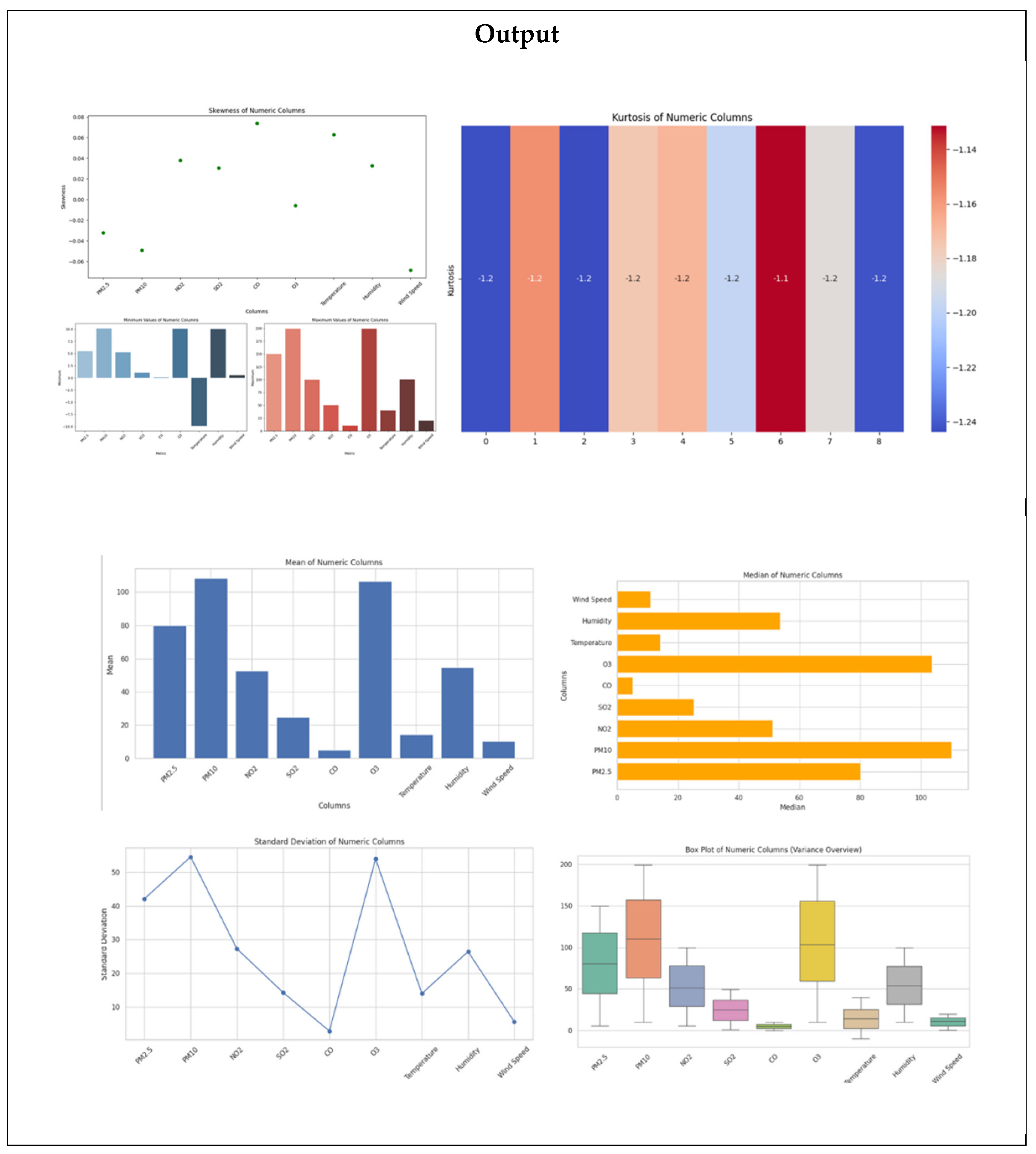
2.2. High-Level Statistics
A meticulous statistical summary of the numerical properties was carried out to ensure data clarity and applicability. Certain significant statistical measures employed are:
Central Tendencies (Mean & Median): The mean is the average numerical variable value, which provides an idea of general pollutant levels and environmental status. The median, however, determines characteristic values and minimizes extreme outliers' influence.
Variability (Standard Deviation & Variance): Standard deviation is a measure of the spread of data from the mean, and it shows variability in pollutant levels and weather conditions. Variance, which is the squared measure of dispersion, adds another level of analysis to data variation.
Range (Minimum & Maximum): Minimum and maximum values of each variable set the range of data, identifying extreme conditions and potential outliers.
Distribution Shape (Skewness & Kurtosis): Skewness measures asymmetry in the data, where positive values indicate right skewness and negative values indicate left skewness. Kurtosis measures the presence of extreme values, which helps in distinguishing between normal and heavy-tailed distributions.
2.3. Data Visualization
Various visualization techniques were adopted to enable data interpretation, including:
Bar Charts to graphically compare mean and range values across numerical features.
Horizontal Bar Charts to represent median values in an alternate manner.
Line Charts to graphically compare standard deviation patterns.
Box Plots to identify variance and possible outliers.
Scatter Plots to graph skewness and symmetry within the dataset.
Side-by-Side Bar Charts to compare minimum and maximum values across numerical columns.
Heatmaps to show differences in kurtosis among different attributes.
2.4. Numeric Data Distributions
To examine the nature of numeric data, the dataset was compared based on different probability distributions:
- Normal Distribution: Describes a symmetrical bell shape, often used to model real-world phenomena.
- Uniform Distribution: Describes equally likely values, suitable for random sampling situations.
- Exponential Distribution: Describes phenomena with high rates of decay and rare extreme values, often used in reliability and survival analysis.
These data visualizations and insights give a general understanding of the data set, providing the opportunity for further exploration into air quality trends and environmental factors.
Figure 1.
High Level Statistics.
3. Literature review
Environmental concerns related to air quality are central to the broader issues of global warming and climate change. Increases in greenhouse gas (GHGs) and other air pollutants such as Particulate Matter (PM2.5, PM10), Nitrogen Dioxide (NO2), Sulfur Dioxide (SO2), Carbon Monoxide (CO), and Ozone (O3) are responsible for deteriorating the environment. Not only do these harmful substances increase the severity of air pollution but also accelerate global warming by increasing the greenhouse effect[11,12].
Urbanization and industrialization at a rapid rate have led to an exponential growth in air pollutants. This has multiplied the frequency of weather extremes, altered patterns of precipitation, and increased surface temperatures. Moreover, urban areas have heightened levels of pollutants from car exhausts and industrial effluents, impacting environmental and human health[13,14,15].
Air pollution also has severe consequences on human health, particularly the respiratory and cardiovascular systems. Repeated exposure to PM2.5 raises the risk of chronic respiratory disease, lung cancer, and cardiovascular disease. Exposure to NO2 is also strongly related to the prevalence of asthma, particularly among children and elderly people[16,17,18].
Certain recent epidemiological evidence suggests that overexposure to atmospheric pollution can lead to increased premature death. Approximately 7 million premature deaths annually are caused by air pollution. The effects are more apparent in densely populated areas, where the levels of pollution surpass safe levels approved by environmental authorities[19,20].
Efforts towards regulating air pollution have been well studied, with numerous means proposed to suppress emissions and improve air quality. The application of renewable energy has been identified as a critical success factor. Replacing filthy sources of energy with cleaner sources, such as solar energy and wind power, can reduce greenhouse gas emissions and improve air quality by a significant margin.
Urban planning steps also has a significant role to play. Smart city initiatives that include green spaces and pollution-minimizing transport systems have been shown to decrease the levels of pollution. Additionally, air quality monitoring systems and policy interventions have been enhanced in most nations to control industrial pollutants and vehicular emissions[21,22].
Advances in technology have permitted real-time air quality monitoring, enhancing pollution control measures. The development of Internet of Things (IoT)-based air quality sensors has facilitated accurate monitoring of pollutants. The application of sensor networks in cities helps authorities take immediate action based on pollution peaks. Artificial intelligence (AI) and machine learning models are also utilized for predictive air quality analysis. AI-based forecasting models can predict pollution levels with high accuracy, which assists policymakers in designing preventive measures. The growing concern regarding air pollution and its adverse effects on climate and health needs immediate attention. Literature stresses the need for stringent regulatory policies, technological advancement, and green urban planning in mitigating the pollution levels. Future research needs to focus on developing more accurate predictive models and exploring new pollution control strategies to protect a healthier and more sustainable environment[23,24].
4. Proposed Methodology
The methodology proposed for this study is designed to facilitate an extensive and organized study of research questions. The study will first carry out a comprehensive review of literature to build a theoretical base, determine research gaps, and narrow the scope of the study. The review will involve current scholarly literature, industry publications, and applicable case studies[25,26,27]. Thereafter, a research design will be developed, involving qualitative and quantitative research approaches, as needed by the study.
The process of data collection will involve primary and secondary sources of data. Primary data will be gathered through organized surveys, interviews, or experiments on a certain population relevant to the research. Sample size and selection will be determined on statistical significance and research feasibility. Secondary data will be obtained from available databases, reports, and previous studies, and hence it will be valid and reliable.
Once data has been collected, it will be pre-processed through cleaning, transformation, and normalization if required. More sophisticated analysis techniques such as statistical analysis, machine learning algorithms[28,29,30], or qualitative coding would be employed for meaningful insights. The steps will provide proper utilization of appropriate tools such as SPSS, Python, R, or other specialized software based on the research requirement[31].
Confirmation of results will be carried out through cross-validation techniques, peer review, or comparative analysis against prevailing benchmarks. Ethical research practices like informed consent, privacy of data[32], and adherence to prevailing research ethics guidelines will be applied rigorously in the course of the research. Finally, the results will be analysed, contextualized, and presented in formalized terms, contributing to the broader academic and business discourse[33].
3.1. Identification of Data Issues
a) Handling Missing Values
Missing values in a data set are of great concern to data analysis since they can compromise statistical inference, cause bias in parameter estimation, and affect sample representativeness. Therefore, identification and treatment of missing values are a critical aspect of data preprocessing.
Implementation Steps:
i) Missing values in all of the columns were examined with data.isnull().sum() and followed by a print statement for any missing values that may be located. Upon execution, there were no missing values found in this data.
ii) To further ensure data integrity, the missing values were computed as a percentage via a percentage formula. A column-dropping function was included to drop any high missing value columns. No columns were dropped because no missing values were present.
iii) Although there were no missing values, steps were taken to address potential issues. Specifically, for numerical columns, missing values (if any) would have been replaced by the mean, while categorical columns would have been replaced by the mode. One last check was performed to confirm that there were no missing values remaining after imputation.
b) Handling Duplicates
Duplicate values can damage data integrity and analysis accuracy. Duplicate detection and handling yield a cleaner dataset and eliminate redundancy.
Implementation Steps:
i) Duplication checks were conducted initially by using data.duplicated().sum() to detect duplicated entries.
ii) The duplicate entries were removed using data.drop_duplicates().No duplicate records were found in this dataset, but using this function on it ensures that any future duplicate records will be automatically addressed, ensuring dataset quality and consistency.
c) Checking for Zero or Negative Values
The presence of zero or negative numbers in certain datasets, particularly those dealing with environmental or biomedical data, may not be desirable. Negative numbers may be unrealistic, while zero numbers may be subject to secondary examination depending on the domains.
Implementation Steps:
i) The presence of relevant columns within the dataset was validated through the use of the condition if col in data.columns.
ii) The number of negative numbers in each column was calculated through data[col][data[col] < 0].count().
iii) Similarly, the number of zero values was ascertained with data[col][data[col] == 0].count.
iv) The output was printed in the format:
"{{{col}}} - Negative Values: {negative_values}, Zero Values: {zero_values}."
Findings:
There were no negative values for columns relating to pollutants (PM2.5, PM10, NO2, SO2, CO, O3), and as anticipated, pollutants have no negative concentrations.
There were zero values in some columns, which while not necessarily invalid, require closer inspection. They may indicate genuinely low levels of contaminants or missing data recorded as zeros. A domain specialist was recommended to determine if the zero records were valid.
3.2. Data Preprocessing Techniques
Preprocessing is an essential step towards the cleaning of raw data to make it ready for analysis. It helps to identify and rectify inconsistencies, giving the dataset a clean, well-organized, and ready-to-reflect state for further processing.
General Steps in Preprocessing:
Data Acquisition
Importing the Libraries Needed
Loading the Dataset
Handling Missing Values and Other Data Problems
Encoding Categorical Variables
Scaling the Features
Partitioning the Dataset for Model Training and Testing
For this dataset, multiple preprocessing techniques were applied, including missing value handling, categorical encoding, duplicate removal, feature scaling, feature engineering, and visualization techniques to identify skewness, outliers, and patterns.
a) Encoding Categorical Data
Machine learning models operate on numeric data, so categorical variables have to be converted into numeric formats.
Implementation Steps:
The original data types of every column were obtained using data.dtypes, which provided a column type summary.
ii) Data Type Conversion:
Date Columns: The date column was converted from object to datetime64[ns] via pd.to_datetime().
Categorical Columns: Categorical variables (for example, City and Country) were transformed from object to the category data type.
b) Feature Scaling
Feature scaling normalizes numerical values into a given range (e.g., 0 to 1 or -1 to 1) in order to prevent any single feature from dominating distance-based algorithms and to improve model performance.
Implementation Steps:
i) Numeric columns were identified using data.select_dtypes(include=np.number).columns.tolist().
ii) Min-Max Scaling:
Min-Max Scaling was applied, which normalizes numerical features to the range of 0–1 without loss of relative structure of the original data. It offers uniform transformation across features and keeps away from bias, along with enhancing the performance of models. All the numerical columns were successfully normalized in the [0,1] range following the use of this method, ensuring data consistency.
c) Feature Engineering
Feature engineering enhances dataset quality by creating new features that capture more insights and improve model interpretability.
Implementation Steps:
i) Feature Interactions Identification:
A new feature, Temp_Humidity_Interaction, was created to identify the interaction between temperature and humidity.
ii) Purpose of the New Feature:
This interaction term is beneficial for environmental data analysis because temperature and humidity both play a role in pollutant dispersion levels. This interaction can improve predictions in environmental modeling.
4. Data Science Techniques
4.1. Used Techniques
i) Exploratory Data Analysis (EDA)
Exploratory Data Analysis (EDA) is a crucial step in understanding the structure, patterns, and key features of a dataset. It helps to detect relationships, inconsistencies, and trends within the data. By performing EDA, we are ensuring appropriate preparation of the dataset to conduct further analysis and modeling activities, and it aids in data preprocessing and model selection.
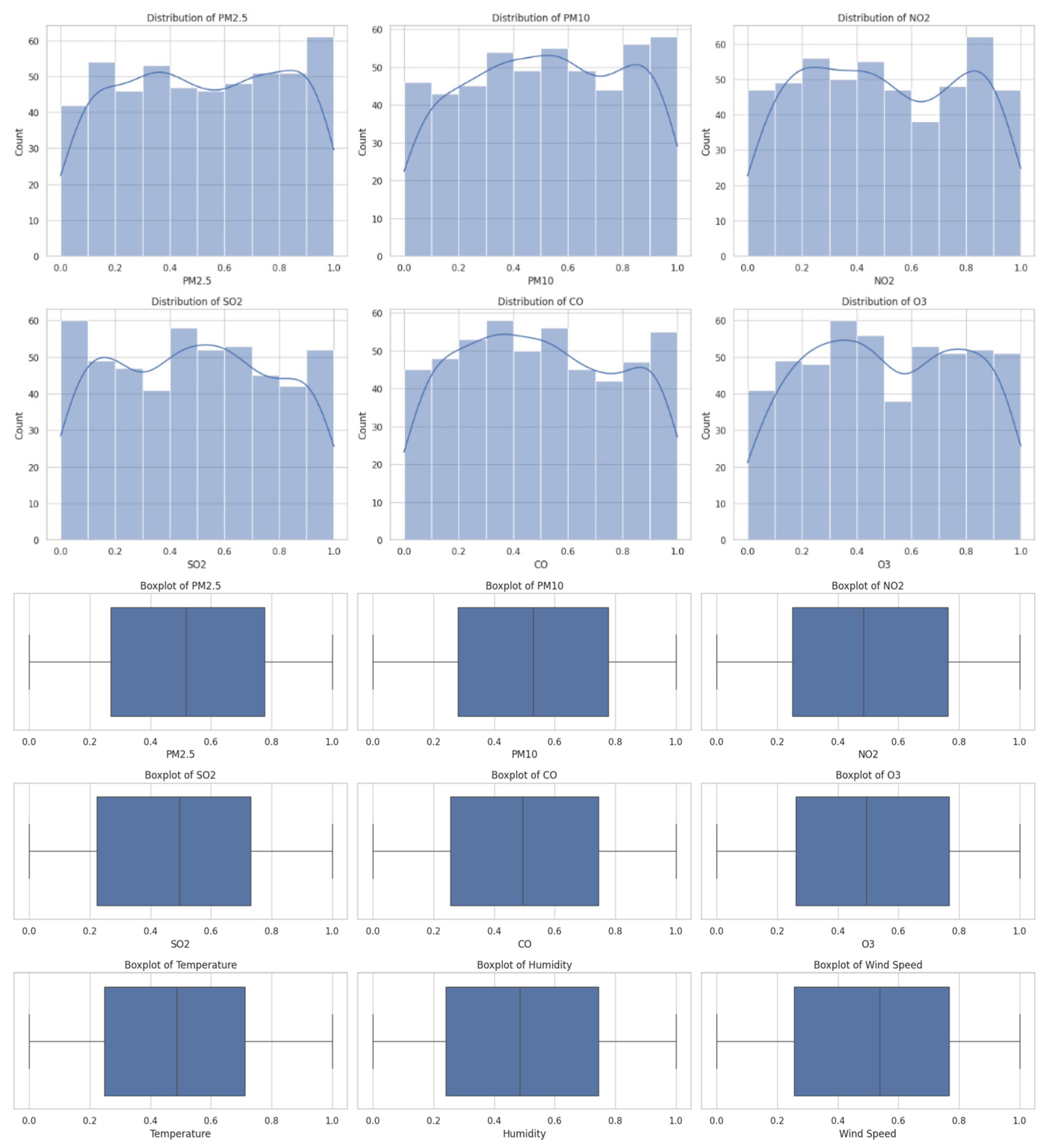
Histograms and Correlation Matrix
Histograms and correlation matrices were employed to depict pollutant concentrations and find patterns in the data. Histograms help determine skewness, variability, and outliers by graphically representing the frequency distribution of values for various pollutant concentrations (PM2.5, PM10, NO2, SO2, CO, and O3). The histograms indicated the distributions of all of the pollutants except PM2.5 were skewed, depicting uneven dispersion with scattered extreme values, which could be indicative of pollution peaks.
Code 10.
Visualize Distributions to Check for Skewness, Outliers, or Patterns.
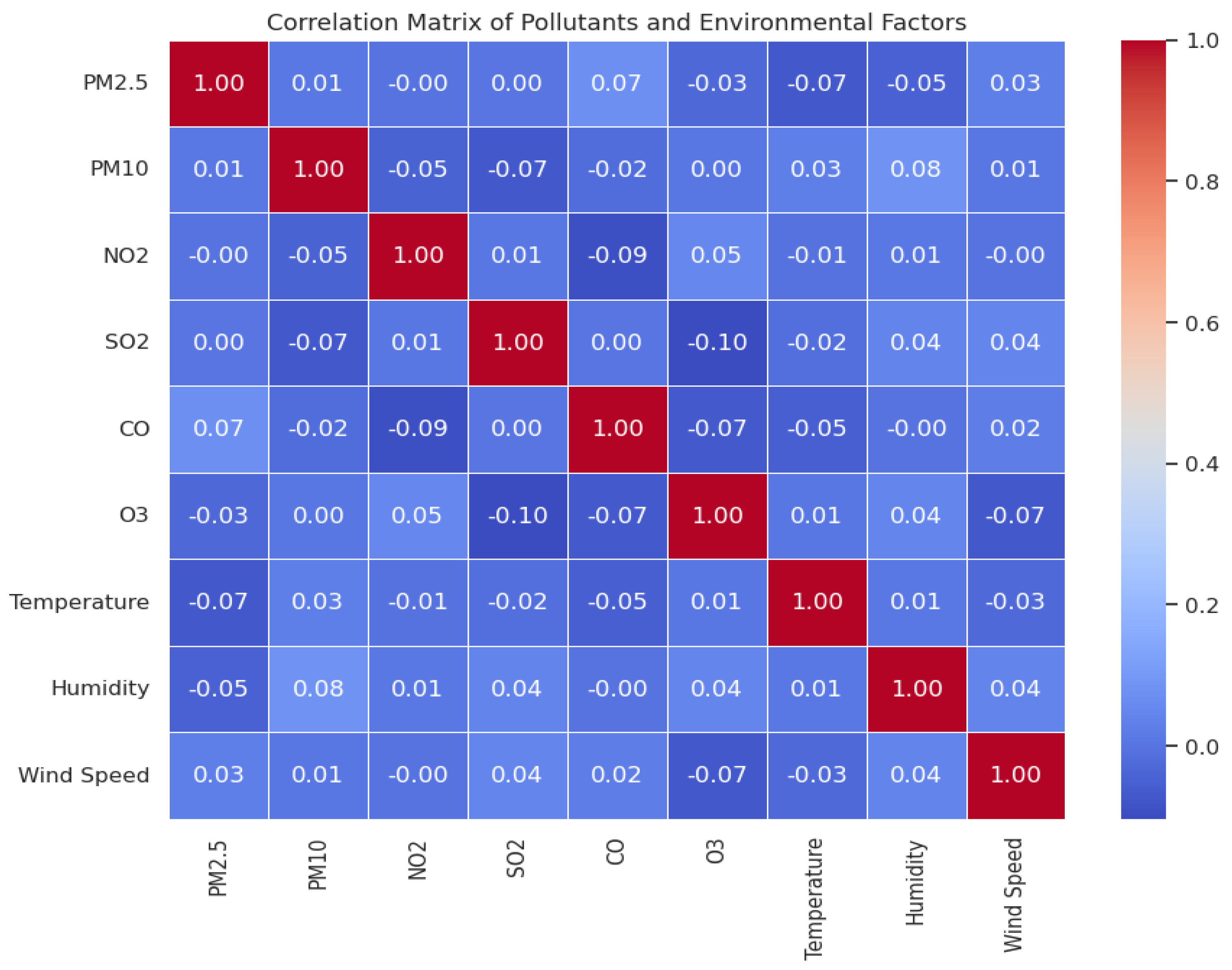
Correlation Matrix
The correlation matrix was utilized to find correlations between environmental variables (temperature, humidity, wind speed) and pollutant levels. A heatmap was utilized to graphically display these relations, which exhibited strong positive correlations between PM2.5 and PM10 as typical indicators of common sources. Weaker relations with environmental variables indicated more subtle or indirect effects.
Code 11.
Correlation Matrix.
ii) Classification analysis:
Classification analysis was done to predict AQI categories such as "Good," "Moderate," "Unhealthy," and "Hazardous" based on pollutant and environmental data. The AQI was computed as a weighted average of PM2.5 and PM10 measurements, with categories assigned based on predefined boundaries. These categories were further translated into numerical labels to ensure machine learning model compatibility.Code 13: Classifying AQI and defining features
Random Forest Classifier:
To classify AQI categories, a Random Forest Classifier was chosen due to its power, ability to handle diverse data types, and performance in recognizing intricate patterns. The model was 1.0 accurate in the test set, reflecting good predictive performance. However, further validation is needed to confirm that the high accuracy is not a case of overfitting or data imbalance.
iii) Regression Model
Regression analysis was utilized to quantify the relationship between environmental parameters and pollutant concentration. Linear Regression modeling was utilized for the estimation of AQI, predicting pollutant concentration on the basis of meteorological properties such as temperature, humidity, and wind speed. The model aimed to identify a best-fit line with minimal error between the predicted and observed values.
For the prediction of AQI, pollutant concentration and environmental conditions were employed as features of interest. These included gaseous pollutants such as particulate matter (PM2.5, PM10), nitrogen dioxide (NO₂), sulfur dioxide (SO₂), carbon monoxide (CO), and ground-level ozone (O₃). Meteorological parameters such as temperature, humidity, and wind speed were also employed. These independent variables were assumed to have a significant influence on AQI, which was employed as the dependent variable.
The data was divided into test and training sets in an 80:20 ratio in order to give the model sufficient data for learning while also reserving some for testing. Random_state = 42 was used for the purpose of reproducibility during splitting.
A Linear Regression model was trained on the training data to discover relationships between the independent variables (features) and the dependent variable (AQI). The model was attempting to minimize the difference between actual and predicted values, improving estimation accuracy.
Also, diagnostic tests such as residual plots and test of residual distribution were conducted to quantify model fit. The tests confirmed that the residuals were spread out at random, a fact which confirmed that the assumptions of the model were tenable.
Rationale for Technique Selection
The techniques used in the project were carefully selected based on the nature of the data, purposes of the analysis, and desired outcomes. Each of the techniques was significant for different phases of the analytical process, offering a complete and correct prediction.
4. Model Validation
4.1. Evaluation Metrics
Regression metrics are numerical measurements to measure the performance of a regression model. Scikit-learn offers some evaluation metrics with their strengths and weaknesses to compare how well a model fits data.
4.2. Types of Regression Metrics
Mean Squared Error (MSE): One of the most frequently used measures across statistics and machine learning, MSE approximates the average of the squared differences between predicted and actual values. MSE approximates the size of the prediction errors, with lower values indicating better model performance. MSE is particularly useful for evaluating regression models and determining prediction accuracy.
R-squared (R²) Score: Also known as the coefficient of determination, R² is a statistical measure that determines the goodness of fit of a regression model to account for the variation in the dependent variable. It calculates the proportion of variance in the dependent variable that can be accounted for by the independent variables. The higher the R², the better the explanatory power and overall model performance.
4.3. Confusion Matrix
Confusion matrix is a performance measurement tool that is primarily used in classification problems. It provides a general breakdown of a model's predictions for all possible classes. For AQI classification, the confusion matrix is utilized to display the relationship between actual AQI classes and the predicted classes by the model graphically.
Each column of the matrix has the predicted category, and each row has the true category. This allows for a more in-depth evaluation of the model's accuracy of classification and to identify misclassifications.
The above code calculates a confusion matrix after it has gone through a categorization function to transform real (y_test) and predicted (y_pred) AQI values into categorical labels. Categorizing the continuous AQI values into discrete categories such as "Good," "Moderate," "Unhealthy," and "Hazardous" makes the results easier to understand.
All 100 test cases fall under the "Good" category with no misclassifications, giving a perfect accuracy value of 1.0. While this is a high accuracy, it also poses a possible issue—the model was possibly trained on an imbalanced dataset, predominantly made up of "Good" AQI values. The absence of other categories ("Moderate," "Unhealthy," and "Hazardous") in actual and predicted values also suggests this direction.
6. Conclusion and Discussion
This project was successful in analyzing air quality from the "Global Air Quality" data set through data cleaning and enrichment, EDA and appropriate modeling techniques. The models developed were found to offer valuable insights into the correlation between pollutants and the environment.
The experiments showed that the Random Forest Classifier achieved very high accuracy in classifying AQI classes, which has to be due to the good working in managing mixed data types and feature interactions. The Linear Regression model gave a good estimate of pollutant concentrations; the analysis also indicated an appreciation of linear correlation between environmental parameters and pollutants. Early statistical results are presented that contain basic correlations between the variables where, for example, PM2.5 is correlated with PM10 Positive and clear definitions of the data distribution and outliers and observable trends. Another issue that can be seen is that due to a small and limited dataset the results cannot be easily generalized. Future research needs to work with more varied datasets from various locations and time frames. Although the accuracy of the classification model is higher according to the results obtained, it has the disadvantage of creating an imbalanced data problem. Another validation with a balanced dataset is recommended so that one has the highest confidence in a specific model. Regression analysis fares poorly with nonlinearity and stochasticity of some air quality parameters because the assumptions of leaning are of a linear relationship.
References
- Freire, P.; Srivallapanondh, S.; Spinnler, B.; Napoli, A.; Costa, N.; Prilepsky, J.E.; Turitsyn, S.K. Computational complexity optimization of neural network-based equalizers in digital signal processing: A comprehensive approach. Journal of Lightwave Technology 2024, 42, 4177–4201. [Google Scholar] [CrossRef]
- Tang, X.; Wang, Z.; Cai, X.; Su, H.; Wei, C. Research on heterogeneous computation resource allocation based on data-driven method. In Proceedings of the 2024 6th International Conference on Data-driven Optimization of Complex Systems (DOCS); 2024; pp. 916–919. [Google Scholar] [CrossRef]
- Ding, H.; Huang, Q.; Alkhayyat, A. A computer aided system for skin cancer detection based on Developed version of the Archimedes Optimization algorithm. Biomedical Signal Processing and Control 2024, 90, 105870. [Google Scholar] [CrossRef]
- Dwivedi, R.; Awasthi, D.; Srivastava, V.K. An optimized dual image watermarking scheme based on redundant DWT and randomized SVD with henon mapping encryption. Circuits, Systems, and Signal Processing 2024, 43, 408–456. [Google Scholar] [CrossRef]
- Abdullah, A. Investigation of brain cancer with interfacing of 3-dimensional image processing. Indian Journal of Science & Technology 2019, 12, 1–12. [Google Scholar]
- Saeed, S.; Khan, H. Global mortality rate and statistical results of Coronavirus. Infectious Diseases and Tropical Medicine 2021, 1–12. [Google Scholar]
- Hayes, B.; Shier, J.; Fazekas, G.; McPherson, A.; Saitis, C. A review of differentiable digital signal processing for music and speech synthesis. Frontiers in Signal Processing 2024, 3, 1284100. [Google Scholar] [CrossRef]
- Jurdana, V. Local Rényi entropy-based Gini index for measuring and optimizing sparse time-frequency distributions. Digital signal processing 2024, 147, 104401. [Google Scholar] [CrossRef]
- Liu, H.; An, J.; Ng, D.W.K.; Alexandropoulos, G.C.; Gan, L. DRL-based orchestration of multi-user MISO systems with stacked intelligent metasurfaces. In Proceedings of the ICC 2024-IEEE International Conference on Communications; 2024; pp. 4991–4996. [Google Scholar] [CrossRef]
- Dogra, V.; Singh, A.; Verma, S.; Kavita, J.N.Z.; Talib, M.N. Analyzing DistilBERT for sentiment classification of banking financial news. In Intelligent Computing and Innovation on Data Science; Peng, S.L., Hsieh, S.Y., Gopalakrishnan, S., Duraisamy, B., Eds.; Springer, 2021; Volume 248, pp. 665–675. [Google Scholar] [CrossRef]
- Alkinani, M.H.; Almazroi, A.A.; Jhanjhi, N.Z.; Khan, N.A. 5G and IoT-based reporting and accident detection (RAD) system to deliver first aid box using unmanned aerial vehicle. Sensors 2021, 21, 6905. [Google Scholar] [CrossRef]
- Babbar, H.; Rani, S.; Masud, M.; Verma, S.; Anand, D.; Jhanjhi, N. Load balancing algorithm for migrating switches in software-defined vehicular networks. Computational Materials and Continua 2021, 67, 1301–1316. [Google Scholar] [CrossRef]
- Saeed, S.; Abdullah, A. Combination of brain cancer with hybrid K-NN algorithm using statistical analysis of cerebrospinal fluid (CSF) surgery. International Journal of Computer Science and Network Security 2021, 21, 120–130. [Google Scholar]
- Saeed, S.; Abdullah, A. Analysis of lung cancer patients for data mining tool. International Journal of Computer Science and Network Security 2019, 19, 90–105. [Google Scholar]
- Saeed, S.; Abdullah, A.; Jhanjhi, N.Z.; Naqvi, M.; Nayyar, A. New techniques for efficiently k-NN algorithm for brain tumor detection. Multimedia Tools and Applications 2022, 81, 18595–18616. [Google Scholar] [CrossRef]
- Saeed, S.; Abdullah, A.; Naqvi, M. Implementation of Fourier transformation with brain cancer and CSF images. Indian Journal of Science & Technology 2019, 12, 1–16. [Google Scholar]
- Shetty, R.; Bhat, V.S.; Pujari, J. Content-based medical image retrieval using deep learning-based features and hybrid meta-heuristic optimization. Biomedical Signal Processing and Control 2024, 92, 106069. [Google Scholar] [CrossRef]
- Yousaf, M.Z.; Singh, A.R.; Khalid, S.; Bajaj, M.; Kumar, B.H.; Zaitsev, I. Enhancing HVDC transmission line fault detection using disjoint bagging and bayesian optimization with artificial neural networks and scientometric insights. Scientific Reports 2024, 14, 23610. [Google Scholar] [CrossRef]
- Du, H.; Wang, J.; Qian, W.; Zhang, X.; Wang, Q. Rotating machinery fault diagnosis based on parameter-optimized variational mode decomposition. Digital Signal Processing 2024, 153, 104590. [Google Scholar] [CrossRef]
- Elshazly, E.A.; El-Shafai, W.; El-Hoseny, H.; El-Rabaie, E.S.M.; Zahran, O.; Abdelwahab, S.A. . & Abd El-Samie, F.E. Software design and FPGA implementation of optimized medical image fusion techniques. Multimedia Tools and Applications 2025, 1–31. [Google Scholar] [CrossRef]
- Hollweg, G.V.; Evald, P.J.D.D.O.; Mattos, E.; Borin, L.C.; Tambara, R.V.; Montagner, V.F. Optimized parametrization of adaptive controllers for enhanced current regulation in grid-tied converters. International Journal of Adaptive Control and Signal Processing 2024, 38, 200–220. [Google Scholar] [CrossRef]
- Thamma, S.R. A Comprehensive Evaluation and Methodology on Enhancing Computational Efficiency through Accelerated Computing. 2024.
- Ismail, N.A.; Khadra, S.A.; Attiya, G.M.; Abdulrahman, S.E.S. Optimizing SIKE for blockchain-based IoT ecosystems with resource constraints. The Journal of Supercomputing 2025, 81, 1–44. [Google Scholar] [CrossRef]
- Li, W.X.; Wang, C.; Wei, H.; Hou, S.; Cao, C.; Pan, C.; Wen, K. Unified Sparse Optimization via Quantum Architectures and Hybrid Techniques. Quantum Science and Technology 2025. [Google Scholar] [CrossRef]
- Aldughayfiq, B.; Ashfaq, F.; Jhanjhi, N.Z.; Humayun, M. Explainable AI for retinoblastoma diagnosis: Interpreting deep learning models with LIME and SHAP. Diagnostics 2023, 13, 1932. [Google Scholar] [CrossRef] [PubMed]
- Kumar, M.S.; Vimal, S.; Jhanjhi, N.Z.; Dhanabalan, S.S.; Alhumyani, H.A. Blockchain based peer to peer communication in autonomous drone operation. Energy Reports 2021, 7, 7925–7939. [Google Scholar] [CrossRef]
- Aherwadi, N.; Mittal, U.; Singla, J.; Jhanjhi, N.Z.; Yassine, A.; Hossain, M.S. Prediction of fruit maturity, quality, and its life using deep learning algorithms. Electronics 2022, 11, 4100. [Google Scholar] [CrossRef]
- Jena, K.K.; Bhoi, S.K.; Malik, T.K.; Sahoo, K.S.; Jhanjhi, N.Z.; Bhatia, S.; Amsaad, F. E-learning course recommender system using collaborative filtering models. Electronics 2022, 12, 157. [Google Scholar] [CrossRef]
- Gill, S.H.; Razzaq, M.A.; Ahmad, M.; Almansour, F.M.; Haq, I.U.; Jhanjhi, N.Z.; Masud, M. Security and privacy aspects of cloud computing: A smart campus case study. Intelligent Automation & Soft Computing 2022, 31, 117–128. [Google Scholar]
- Muzafar, S.; Jhanjhi, N.Z. Success stories of ICT implementation in Saudi Arabia. In Employing Recent Technologies for Improved Digital Governance; IGI Global. 2020; pp. 151–163.
- Alferidah, D.K.; Jhanjhi, N.Z. Cybersecurity impact over bigdata and iot growth. In Proceedings of the 2020 International Conference on Computational Intelligence (ICCI); 2020; pp. 103–108. [Google Scholar] [CrossRef]
- Alkinani, M.H.; Almazroi, A.A.; Jhanjhi, N.Z.; Khan, N.A. 5G and IoT based reporting and accident detection (RAD) system to deliver first aid box using unmanned aerial vehicle. Sensors 2021, 21, 6905. [Google Scholar] [CrossRef]
- Shah, I.A.; Jhanjhi, N.Z.; Laraib, A. Cybersecurity and blockchain usage in contemporary business. In Handbook of Research on Cybersecurity Issues and Challenges for Business and FinTech Applications; IGI Global: 2023; pp. 49–64.
Disclaimer/Publisher’s Note: The statements, opinions and data contained in all publications are solely those of the individual author(s) and contributor(s) and not of MDPI and/or the editor(s). MDPI and/or the editor(s) disclaim responsibility for any injury to people or property resulting from any ideas, methods, instructions or products referred to in the content. |
© 2025 by the authors. Licensee MDPI, Basel, Switzerland. This article is an open access article distributed under the terms and conditions of the Creative Commons Attribution (CC BY) license (http://creativecommons.org/licenses/by/4.0/).
Copyright: This open access article is published under a Creative Commons CC BY 4.0 license, which permit the free download, distribution, and reuse, provided that the author and preprint are cited in any reuse.


