
Submitted:
20 January 2025
Posted:
21 January 2025
You are already at the latest version
Abstract
A multi-TeV Muon Collider produces a significant amount of Higgs bosons allowing precise measurements of its couplings to Standard Model fundamental particles. Moreover, Higgs boson pairs are produced with a relevant cross-section, allowing the determination of the second term of the Higgs potential by measuring the double Higgs production cross section and therefore the trilinear self-coupling term. This contribution aims to give an overview of the Higgs measurements accuracies expected for the initial stage of the Muon Collider at s=3TeV with an integrated luminosity of 1ab−1 and for the target center-of-mass energy at 10TeV with 10ab−1 integrated luminosity. The results are obtained using the full detector simulations which include both physical and machine backgrounds.
Keywords:
muon
; collider
; higgs
; HEP
1. Introduction
The discovery of the Higgs boson at the Large Hadron Collider (LHC) confirmed the mechanism of electroweak symmetry breaking and mass generation in the Standard Model (SM). While the measured properties of the Higgs boson are consistent with SM predictions, significant open questions remain. These include the exact nature of the Higgs potential, the strength of its self-couplings, and the potential presence of new physics beyond the SM. The couplings of the Higgs boson with SM particles have been measured at the LHC, but achieving sub-percent precision is essential to explore potential deviations from the SM [1]. Furthermore, the trilinear () and quadrilinear () Higgs self-couplings, which are critical for probing the Higgs potential, cannot be observed in current experiments due to the low cross section of multi-Higgs processes [2]. At a multi-TeV Muon Collider, a significant number of Higgs bosons, summarized in Table 1, could be produced through fusion in the process enabling detailed studies of their couplings. Moreover processes such as and could be observed to measure and [3].
Thus, the Muon Collider provides a unique opportunity to meet the physics requirements for next generation particle accelerators. It combines the clean environment of a lepton machine with the capability of reaching very high collision energies as a hadron machine, thanks to the low synchrotron radiation losses of muon beams. However, the unstable nature of the muon introduces several technical challenges that must be addressed for both the machine and detectors to establish the feasibility of such a collider.
2. Beam-Induced Background (BIB)
One of the primary challenges associated with the Muon Collider arises from the intrinsic instability of muons. They decay in the beam pipe, and the resulting decay products interact with the collider components, generating a flux of photons, neutrons, and charged particles that reach the detector, known as Beam-Induced Background (BIB) [4]. Effective mitigation strategies are essential to reduce BIB and ensure the desired detector performance and measurement accuracy. These include both hardware and software approaches. In particular in the Machine-Detector Interface (MDI) design includes two tungsten, cone-shaped shielding (nozzles) located along the beamline inside the detector area to minimize the number and the energy of the incoming particles. Moreover, the reconstruction algorithm will be tuned to handle the combinatorial noise coming from the BIB, exploiting advanced 5D sensors, which are capable of measuring energy, position, and timing with very high resolution. In particular, the time of arrival in the detector is a crucial information since a large fraction of BIB is asynchronous to the bunch crossing, as shown in Figure 1. A prototype detector design, along with specialized reconstruction algorithms, has already been developed for a Muon Collider at [5,6]. The detector and MDI optimization for the case is in progress [7].
3. Higgs Cross Section
This section presents the sensitivity estimates for measuring the cross-sections of Higgs boson decays into various channels at a center-of-mass energy of at a Muon Collider. The analysis was conducted following these steps:
-
Monte Carlo Event Generation: The Higgs decay modes considered in this study include:
- -
- ,
- -
- ,
- -
- ,
- -
- ,
- -
- .
Signal events were generated at leading order using the Monte Carlo event generators MadGraph5_aMC@NLO [8] (referred to hereafter as MadGraph) and WHIZARD2[9]. Particle showering and hadronization were handled with PYTHIA version 8.200. For each decay mode, the corresponding background processes were also simulated. The complete list of generated samples is provided in Appendix A. - Detector Simulation: A detailed detector simulation was carried out using GEANT4[10]. The detector incorporates advanced silicon-based tracking systems, electromagnetic and hadronic calorimeters, and operates within a 3.57 T magnetic field. Beam-Induced Background (BIB) was overlaid at the hit level, and digitization was applied to simulate sensor responses with realistic timing and spatial resolutions. The detector model is shown in Figure 2.
-
Determination of the Sensitivity: The sensitivity on the cross-section for each Higgs decay mode was derived from the sensitivity on the number of events using the relation:where is the luminosity, is the efficiency, and is the cross-section. The sensitivity on was determined by propagating the sensitivity on the number of events, assuming negligible uncertainties on the luminosity and efficiency.For , the cross-section was determined by fitting the di-jet invariant mass distributions of signal and background using double-Gaussian functions to model the signal and background. A likelihood function was constructed with these models, and an unbinned maximum-likelihood fit was performed on pseudo-data. The signal and background yields were allowed to float to extract the yield and its uncertainty. The uncertainty on the cross-section was estimated by averaging over several pseudo-experiments. The result is shown in Table 2.For the other signals considered in this study, the statistical sensitivity on the cross-section was determined using a counting experiment. Assuming negligible uncertainties on the efficiency and integrated luminosity, the relative error on is given by:where S and B are the expected numbers of signal and background events, respectively. To maximize the signal-to-background ratio, machine learning algorithms such as Boosted Decision Trees (BDTs)[14] and Multi-Layer Perceptrons (MLPs)[15] were trained on physical observables specific to each signal process and used as discriminators. The results are presented in Table 2. The table also includes results obtained with fast simulation performed with Delphes cards[16] without incorporating BIB[17]. The two estimates are in very good agreement, indicating that BIB effects on physics performance are manageable.
4. Double Higgs Cross Section
Double Higgs events will be produced at a Muon Collider through processes reported in Figure 3.
Following the procedure outlined in Section 3, the expected precision on the measurement of the double Higgs boson production cross section has been estimated. For this analysis, only the decay channel has been considered for both Higgs bosons, given the limited contribution from other decay modes [18,19]. However, further studies will include additional channels such as and .
The reconstruction of events begins by forming all possible two-jet combinations, requiring at least one jet in each pair to be tagged as a b-jet. Higgs boson candidates are identified by selecting the jet pairs whose invariant masses, and , minimize the figure of merit:
where is the known Higgs boson mass.
The primary background in this analysis arises from processes that produce four heavy-quark jets (), predominantly through the decay of intermediate electroweak gauge bosons. Another significant background stems from , where single Higgs production mimics the signal but lacks the trilinear Higgs coupling.
To suppress these backgrounds, advanced tagging algorithms are used, and light-quark jets or fake jets are assumed to be negligible due to effective vetoing techniques based on jet substructure and machine learning methods. To enhance the separation of the signal from the background, a MLP is trained using the following observables:
- The invariant masses of the two jet pairs;
- The magnitude of the vector sum of the four jet momenta;
- The total energy of the four jets;
- The angle between the two jet pairs relative to the leading candidate;
- The maximum separation angle between jets in the event;
- The angles between the highest- jet in the pair and the leading and sub-leading candidates with respect to the z-axis;
- The transverse momenta of the four jets.
The output of the MLP is shown in Figure 4, demonstrating clear separation between the signal and the dominant background.
Using the MLP output, pseudo-datasets were generated based on the expected event yields. The signal yield was extracted by fitting the MLP distribution. Averaging over pseudo-experiments yielded an uncertainty of .
Since the cross section is directly proportional to the signal yield as described in Eq. 1, and uncertainties in efficiency and luminosity are considered negligible, the sensitivity to the cross section is given by:
5. Trilinear Higgs Coupling
The double Higgs cross section is sensitive to the parameter of the Higgs potential when the production occurs via off-shell Higgs (). The Feynman diagram of the processes is reported on the left in Figure 3.
In order to estimate the sensitivity on the measurement of the following procedure has been adopted:
- Different set of double Higgs events has been generated with WHIZARD varying from 0.2 to 1.8 with 0.2 steps.
- The same MLP used in Section 4 has been exploited to separated the SM signal, corresponding to , from physical background.
- A second MLP has been trained to separate the double Higgs processes via from the other two. The observables considered to perform the discrimination were: the angle between the two Higgs boson momenta in the laboratory frame, the angle between the highest- jet momenta of each pair with respect to the z axis, and the helicity angle of the two Higgs boson candidates.
- The scores of the two MLPs for the considered samples have been arranged in 2-dimensional histograms. To obtain the expected data distribution, 2-dimensional templates of the signal and background components are built for each hypothesis.
- Pseudo-datasets are generated with the total 2D template for the hypothesis. For each pseudo-experiment, the likelihood difference is calculated as a function of by comparing the pseudo-data distribution to the templates.
- The log-likelihood profile has been fitted with a polynomial function of fourth degree. The uncertainty on at 68% Confidence Level (C.L.) is estimated as the interval around where the fitted polynomial has a value below 0.5.
The result obtained with the current algorithms, does not provide an adequate representation of the true potential of Muon Collider for this measurement. However, realistic assumption has been made on the jet tagging efficiency and energy resolution to estimate the uncertainty on the trilinear Higgs self-coupling . Considering a b-tagging efficiency, a -mistag rate and a jet momentum resolution the likelihood scan reported in Figure 5 has been obtained, resulting in sensitivity on of
6. Conclusions
The results presented in this study demonstrate the potential of the Muon Collider operating at a center-of-mass energy of to probe the Higgs sector of the Standard Model with high precision. The agreement between the results obtained using full detector simulations, which account for realistic Beam-Induced Backgrounds, and those derived from fast simulations at supports the validity of the fast simulation methodology.
This consistency allows us to assume that the results from fast simulations for the Muon Collider, shown in Figure 6, provide a realistic representation of its potential. In particular, the case has been considered as a proof of concept for multi-TeV stages. At , objects are more boosted towards the forward region, however, the transverse momentum distribution of objects such as the Higgs boson remains rather similar between and , as shown in Figure 7. This similarity further supports the reliability of fast simulation results for the 10 TeV Muon Collider. The machine emerges as one of the most promising facilities for advancing Higgs boson studies and achieving precision measurements of its properties.
Ongoing efforts are focused on optimizing the detector design and the MDI for the machine. These optimizations will ensure enhanced performance, and detailed results are anticipated to be published by 2025.
Appendix A
Table A1 summarizes all Monte Carlo samples used in this paper. It lists the simulated processes, the generators employed, and the generator-level cuts. The generation requirements are applied to , the transverse momentum with respect to the z axis (where i is the particle type), to the invariant mass of two particles , to the pseudorapidity or to the distance between two particles in the - space, , where is the angle with respect to the x axis in the x-y plane.

Table A1.
Summary of the generated samples indicating the Monte Carlo generator used and the kinematical requirements applied to the final-state particles. M represents the invariant mass of the objects shown in parentheses. The symbol q stands for u, d, s, c, or b quarks, while ℓ stands for electron, muon or tau. Symbol stands for electron, muon or tau neutrino. If is present, all possible combination of quark flavours, even different flavours, are considered by WHIZARD/Madgraph. If the Higgs boson is not indicated in the process, Yukawa couplings are switched off.
| Process | Generator | Kinematical requirements |
|---|---|---|
| WHIZARD | - | |
| WHIZARD | - | |
| WHIZARD | - | |
| WHIZARD | GeV | |
| WHIZARD | GeV | |
| WHIZARD | - | |
| MadGraph | - | |
| WHIZARD | - | |
| WHIZARD | GeV | |
| MadGraph | GeV | |
| MadGraph | GeV, | |
| MadGraph | > 1 GeV, < 3 | |
| > 5 GeV, < 3 | ||
| > 0.2, | ||
| WHIZARD | GeV | |
| WHIZARD | GeV | |
| MadGraph | > 1 GeV, < 3 | |
| > 5 GeV, < 3 | ||
| > 0.2, | ||
| MadGraph | > 10 GeV | |
| > 5 GeV, < 3 | ||
| > 0.2, | ||
| WHIZARD | GeV | |
| WHIZARD | GeV | |
| WHIZARD | GeV | |
| WHIZARD | GeV | |
| WHIZARD | GeV | |
| WHIZARD | GeV | |
| WHIZARD | GeV | |
| WHIZARD | 10 GeV < < 150 GeV | |
| < 2.5, < 2.5 | ||
| > 5 GeV, > 5 GeV | ||
| > 0.3 | ||
| MadGraph | GeV, | |
| MadGraph | GeV, | |
| MadGraph | GeV | |
| Madgraph | GeV, | |
| Madgraph | GeV, | |
| Madgraph | GeV, | |
| Madgraph | GeV, |
References
- de Blas, J.; Cepeda, M.; D’Hondt, J.; Ellis, R.; Grojean, C.; Heinemann, B.; Maltoni, F.; Nisati, A.; Petit, E.; Rattazzi, R.; et al. Higgs Boson studies at future particle colliders. Journal of High Energy Physics 2020, 2020. [Google Scholar] [CrossRef]
- ATLAS.; Collaborations, C. Report on the Physics at the HL-LHC and Perspectives for the HE-LHC, 2019, [arXiv:hep-ex/1902.10229].
- Chiesa, M.; Maltoni, F.; Mantani, L.; Mele, B.; Piccinini, F.; Zhao, X. Measuring the quartic Higgs self-coupling at a multi-TeV muon collider. Journal of High Energy Physics 2020, 2020. [Google Scholar] [CrossRef]
- Lucchesi, D.; Bartosik, N.; Calzolari, D.; Castelli, L.; Lechner, A. Machine-Detector interface for multi-TeV Muon Collider. PoS 2024, EPS-HEP2023, 630. [CrossRef]
- Bartosik, N.; Bertolin, A.; Buonincontri, L.; Casarsa, M.; Collamati, F.; Ferrari, A.; Ferrari, A.; Gianelle, A.; Lucchesi, D.; Mokhov, N.; et al. Detector and Physics Performance at a Muon Collider. Journal of Instrumentation 2020, 15, P05001–P05001. [Google Scholar] [CrossRef]
- Bartosik, N.; Krizka, K.; Griso, S.P.; Aimè, C.; Apyan, A.; Mahmoud, M.A.; Bertolin, A.; Braghieri, A.; Buonincontri, L.; Calzaferri, S.; et al. Simulated Detector Performance at the Muon Collider, 2022, [arXiv:hep-ex/2203.07964]. arXiv:hep-ex/2203.07964].
- Casarsa, M. Detector performance for low- and high-momentum particles in s = 10 TeV muon collisions, 2024. [CrossRef]
- Alwall, J.; et al. The automated computation of tree-level and next-to-leading order differential cross sections, and their matching to parton shower simulations. JHEP 2014, 07, 079–1405.0301. [Google Scholar] [CrossRef]
- Bredt, P.M.; Kilian, W.; Reuter, J.; Stienemeier, P. NLO electroweak corrections to multi-boson processes at a muon collider. JHEP 2022, arXiv:2208.09438]12, 138. [Google Scholar] [CrossRef]
- Agostinelli, S.; et al. Geant4—a simulation toolkit. Nucl. Instrum. Methods A 2003, 506, 250–303. [Google Scholar] [CrossRef]
- Gaede, F. Marlin and LCCD—Software tools for the ILC. Nucl. Instrum. Methods A 2006, 559, 177–180. [Google Scholar] [CrossRef]
- Thomson, M. Particle flow calorimetry and the PandoraPFA algorithm. Nucl. Instrum. Methods A 2009, arXiv:0907.3577]611, 25–40. [Google Scholar] [CrossRef]
- Andreetto, P.; Bartosik, N.; Buonincontri, L.; Calzolari, D.; Candelise, V.; Casarsa, M.; Castelli, L.; Chiesa, M.; Colaleo, A.; Molin, G.D.; et al. Higgs Physics at a s=3 TeV Muon Collider with detailed detector simulation, 2024, [arXiv:hep-ex/2405.19314]. arXiv:hep-ex/2405.19314].
- Roe, B.P.; et al. Boosted decision trees as an alternative to artificial neural networks for particle identification. Nucl. Instrum. Methods A 2005, 543, 577–584. [Google Scholar] [CrossRef]
- Hoecker, A.; et al. TMVA - Toolkit for Multivariate Data Analysis, 2009, [physics/0703039]. [CrossRef]
- de Favereau, J.; et al. DELPHES 3: a modular framework for fast simulation of a generic collider experiment. JHEP 2014, 02, 057–1307.6346. [Google Scholar] [CrossRef]
- Forslund, M.; Meade, P. Precision Higgs Width and Couplings with a High Energy Muon Collider, 2024, [arXiv:hep-ph/2308.02633].
- Buonincontri, L. Study of mitigation strategies of beam-induced background and Higgs boson couplings measurements at a muon collider., 2020.
- Buonincontri, L. Search for heavy flavour Higgs boson decays at hadron and future Muon Collider, 2023.
- Accettura, C.; et al. Towards a Muon Collider. Eur. Phys. J. C 2023, 83, arXiv–2303.08533. [Google Scholar] [CrossRef]
Figure 1.
Arrival times of the main BIB components at the detector relative to the bunch crossing. For (solid) and .
Figure 1.
Arrival times of the main BIB components at the detector relative to the bunch crossing. For (solid) and .
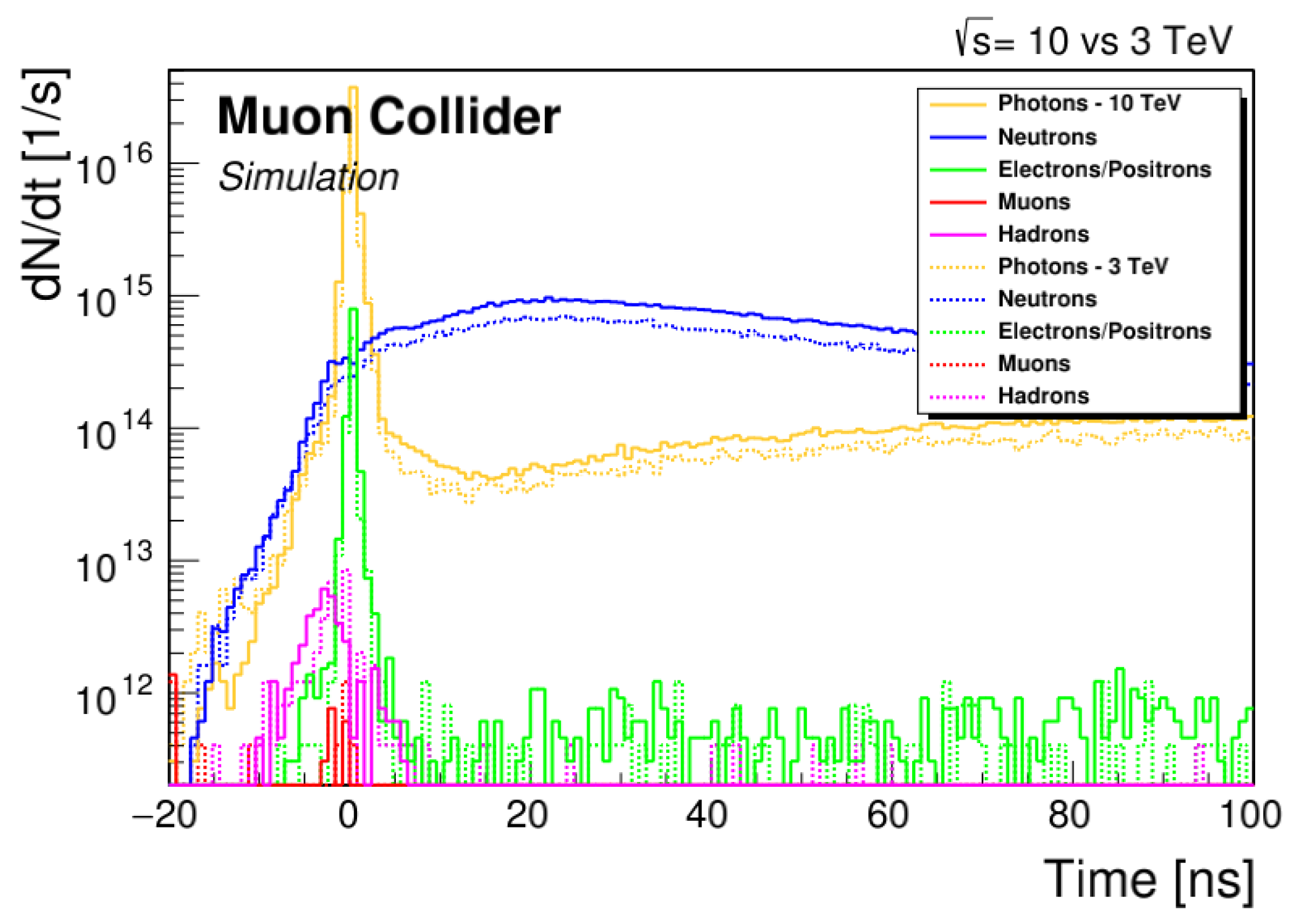
Figure 2.
The detector model used in the detailed simulation, viewed in the y-z plane. From the innermost to the outermost regions, it includes a tracking system (green), an electromagnetic calorimeter (yellow), a hadronic calorimeter (magenta), a superconducting solenoid (light blue), barrel (light green), and endcap (blue) muon detectors. The nozzles are shown in cyan.
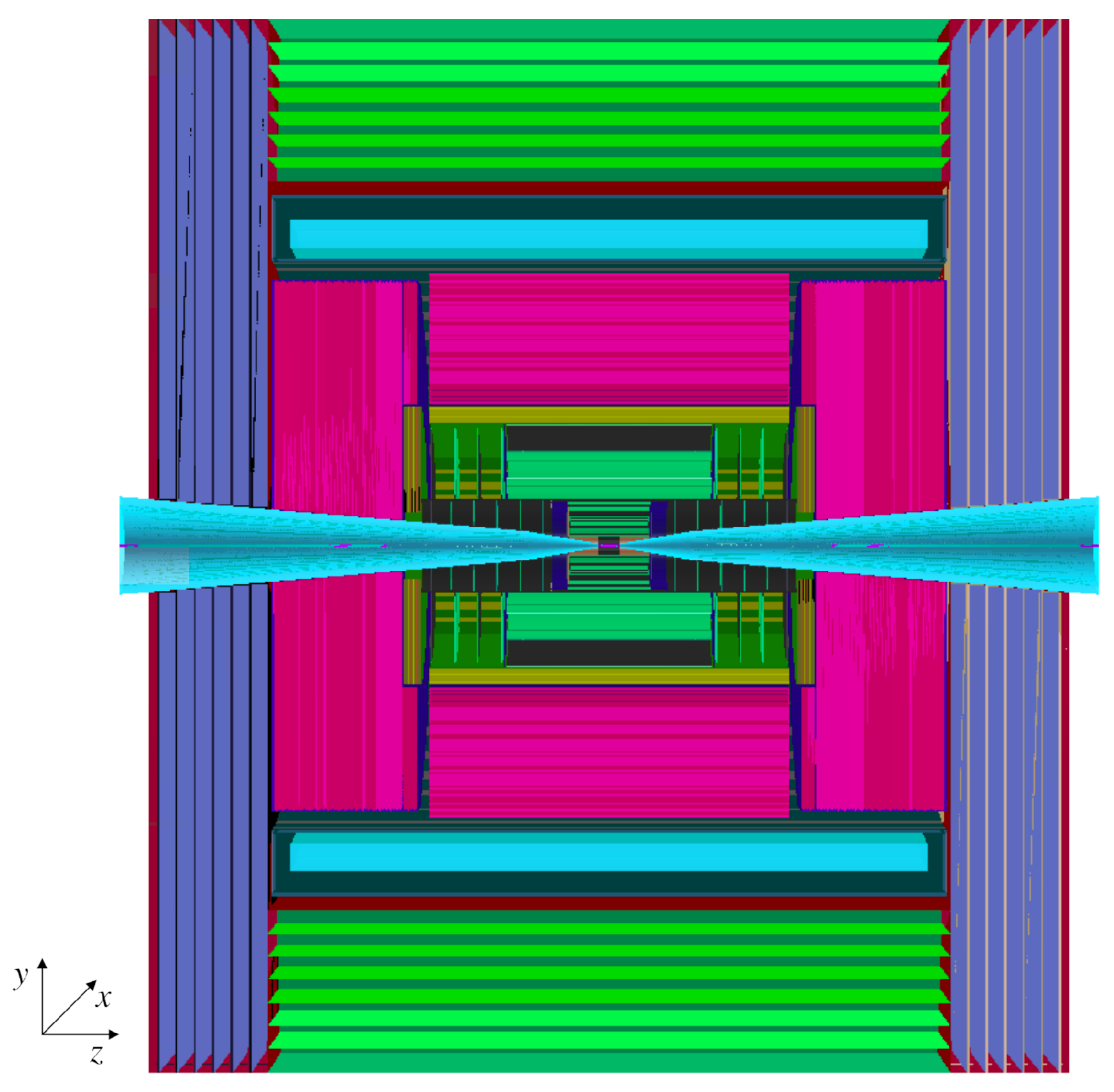
Figure 3.
Feynman tree-level diagrams representing the major contributions to the double-Higgs production at a Muon Collider. The first diagram on the left represents the process directly related to the Higgs self-coupling .
Figure 3.
Feynman tree-level diagrams representing the major contributions to the double-Higgs production at a Muon Collider. The first diagram on the left represents the process directly related to the Higgs self-coupling .
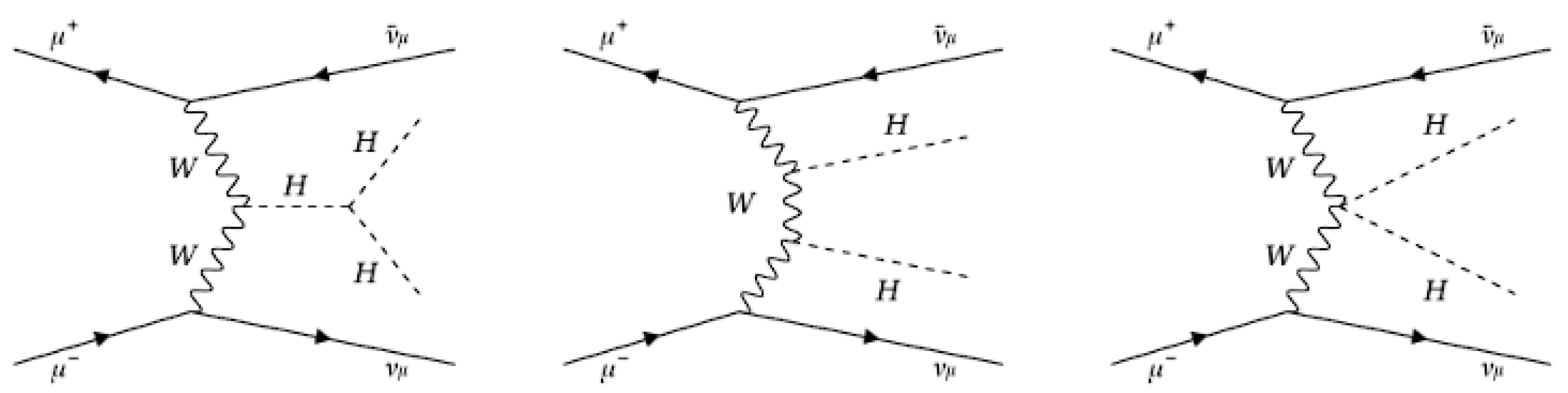
Figure 4.
Distributions of the MLP output for the signal and main background contributions, normalized to unit area.
Figure 4.
Distributions of the MLP output for the signal and main background contributions, normalized to unit area.
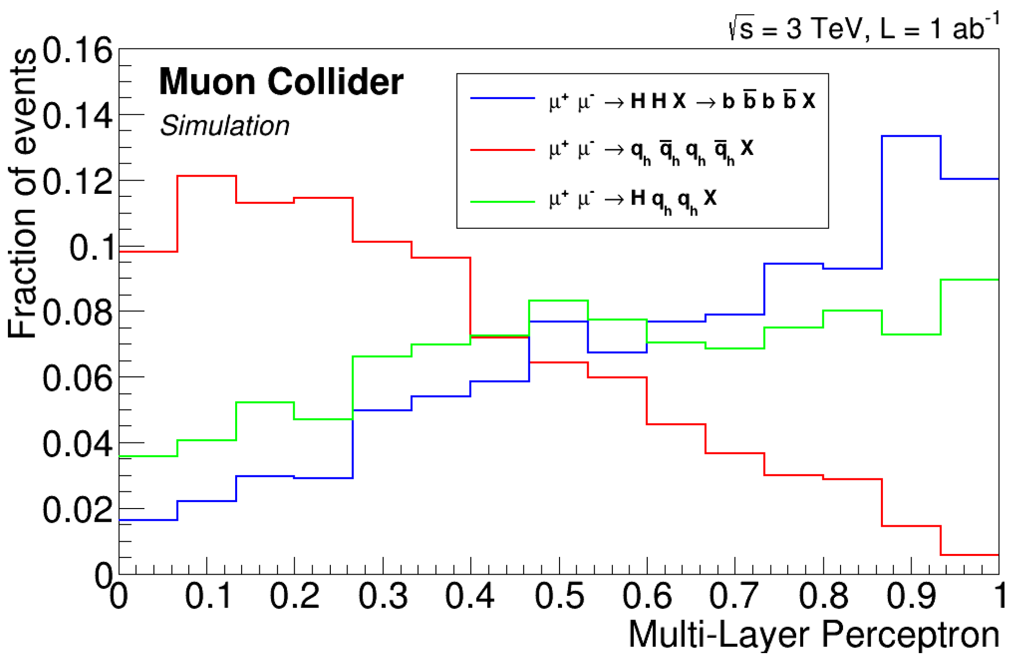
Figure 5.
Likelihood difference () as a function of hypothesis for samples reconstructed without the BIB.
Figure 5.
Likelihood difference () as a function of hypothesis for samples reconstructed without the BIB.
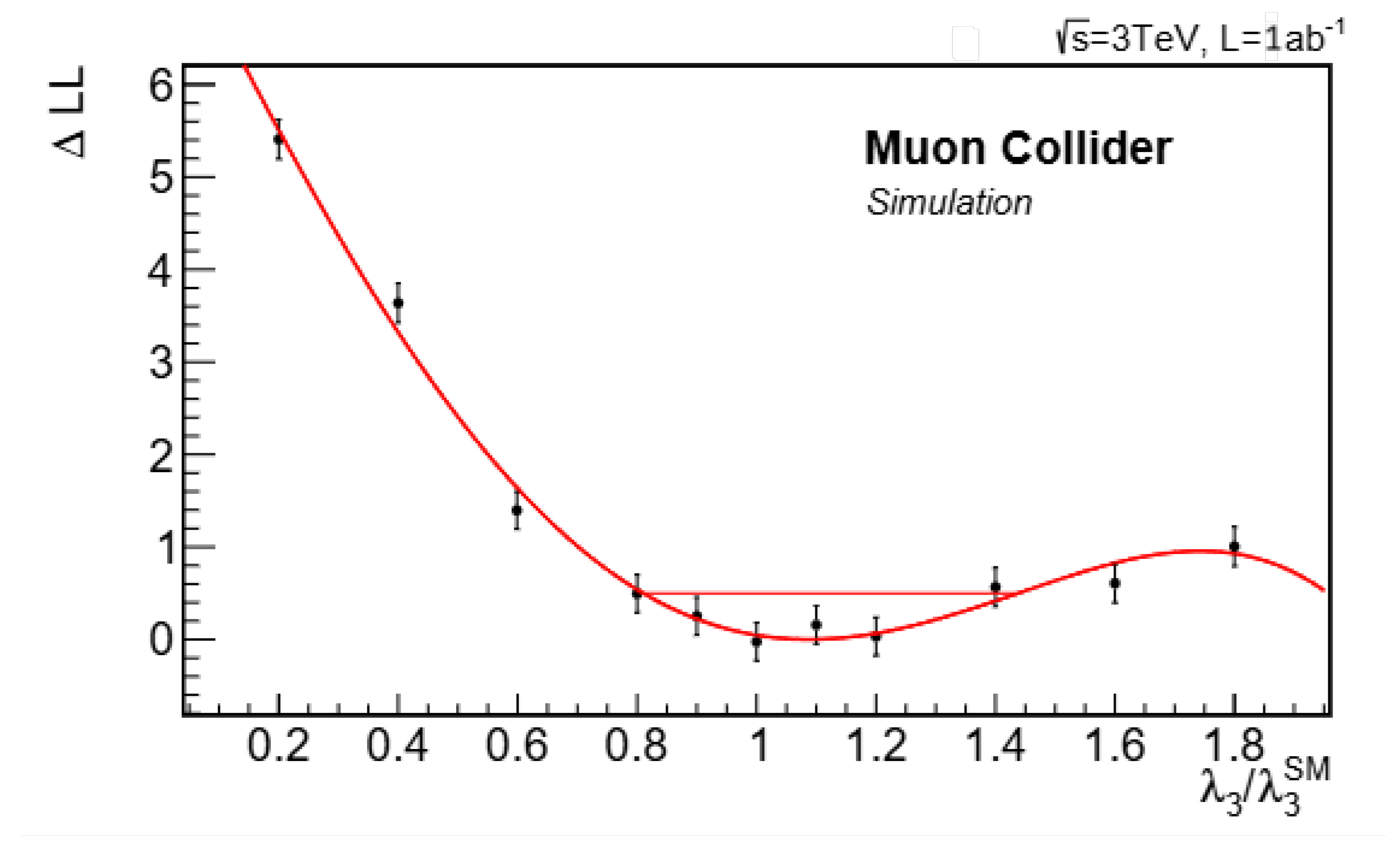
Figure 6.
Comparison of Higgs couplings precision for a and Muon Collider, in combination with expected results coming from HL-LHC.
Figure 6.
Comparison of Higgs couplings precision for a and Muon Collider, in combination with expected results coming from HL-LHC.
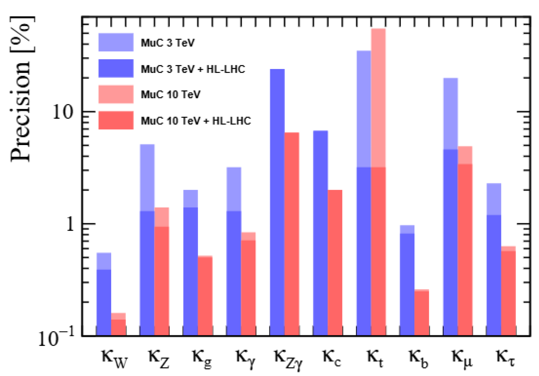
Figure 7.
Higgs boson transverse momentum distribution at (red) and (blue) case.
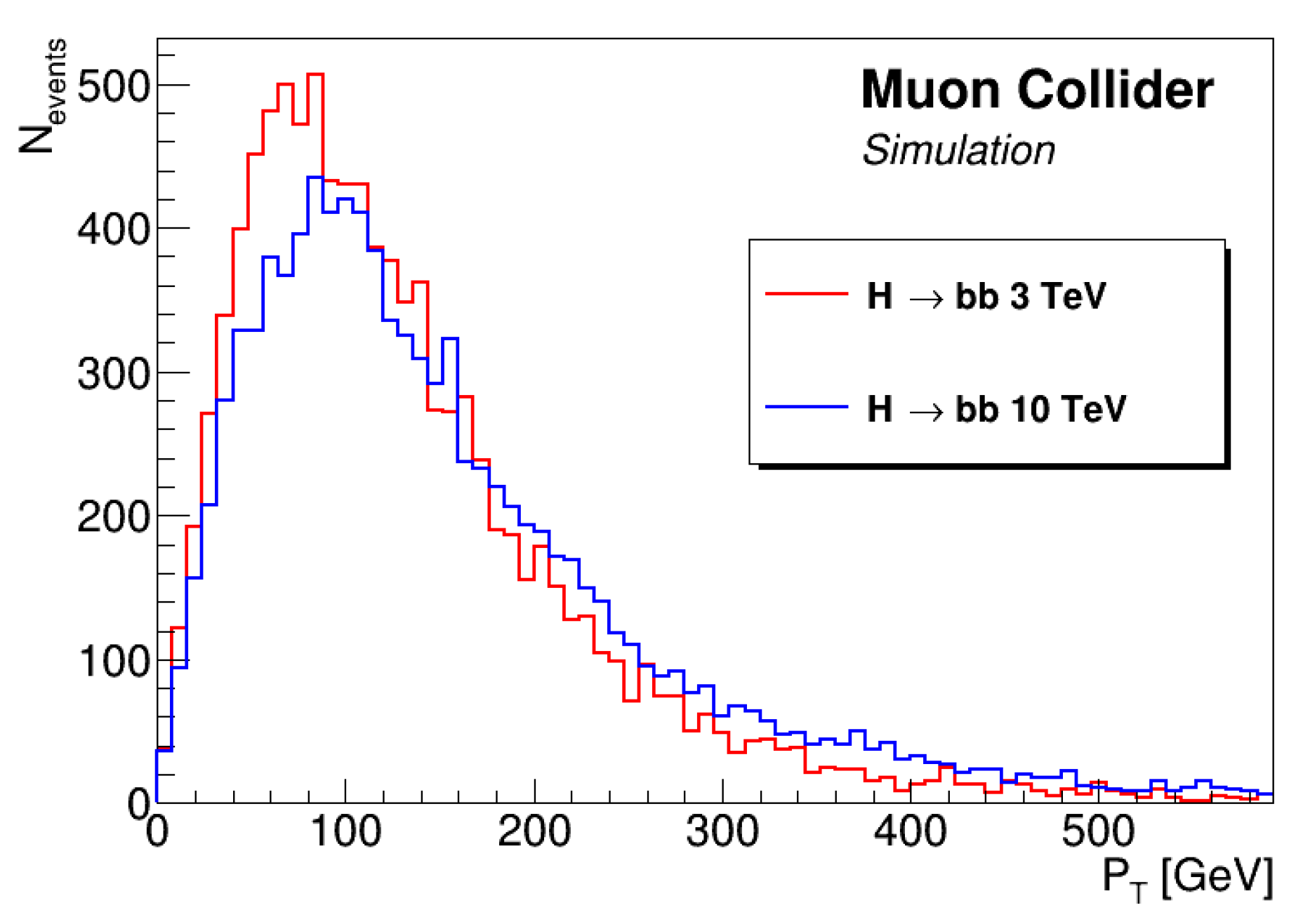
Table 1.
Expected number of Higgs events at different Muon Collider stages.
| C.o.M energy [TeV] | Luminosity [] | Higgs Events |
|---|---|---|
| 3 | 1 | |
| 10 | 10 | |
| 14 | 20 | |
| 30 | 90 |
Table 2.
Expected sensitivities on the cross-sections of Higgs boson decays at Muon Collider obtained with full detector simulation compared to results obtained with fast simulation without including Beam-Induced Background (BIB).
Table 2.
Expected sensitivities on the cross-sections of Higgs boson decays at Muon Collider obtained with full detector simulation compared to results obtained with fast simulation without including Beam-Induced Background (BIB).
| Channel | Full Sim. | Fast Sim. |
|---|---|---|
| 17 | 11 | |
| 39 | 40 | |
Disclaimer/Publisher’s Note: The statements, opinions and data contained in all publications are solely those of the individual author(s) and contributor(s) and not of MDPI and/or the editor(s). MDPI and/or the editor(s) disclaim responsibility for any injury to people or property resulting from any ideas, methods, instructions or products referred to in the content. |
© 2025 by the authors. Licensee MDPI, Basel, Switzerland. This article is an open access article distributed under the terms and conditions of the Creative Commons Attribution (CC BY) license (http://creativecommons.org/licenses/by/4.0/).
Copyright: This open access article is published under a Creative Commons CC BY 4.0 license, which permit the free download, distribution, and reuse, provided that the author and preprint are cited in any reuse.


