
Submitted:
20 January 2025
Posted:
21 January 2025
You are already at the latest version
Abstract
The Coherent Hemodynamic Spectroscopy (CHS) model provides a quantitative framework for modeling cerebral hemodynamics and metabolism, particularly in response to small physiological perturbations. However, in its original approximate formulation it was limited to conditions where parameter changes were constrained to 10–20%, making it unsuitable for modeling extreme physiological disruptions such as cardiac arrest. In this study, we present a detailed discussion of the algorithm using the complete CHS model, which extends the original framework by solving partial differential equations without approximations to handle large non-periodic perturbations. This model was applied to data from a previously published cardiac arrest and cardiopulmonary resuscitation (CPR) study in pigs, where cerebral blood flow changed by 100%. While our prior work demonstrated the utility of this approach for analyzing cerebral microvascular and metabolic parameters, it did not include the algorithmic details necessary for reproducibility and broader application. Here we address this gap by describing the algorithm's workflow, including the use of non-linear multivariate optimization, and its ability to recover multiple physiological variables, such as the capillary and venule oxygen saturations, and parameters, such as the capillary oxygen diffusion rate, and arterial oxygen saturation. The latter can be valuable when the pulse oximetry measurements are unavailable due to unstable, weak or absent pulse. This study underscores the importance of non-linear modeling in advancing the application of CHS to extreme physiological conditions and highlights its potential for translational research and clinical innovation.
Keywords:
Coherent Hemodynamic Spectroscopy
; hemodynamic model
; near-infrared spectroscopy
; NIRS
; brain
; neuronal activity
; cardiac arrest
; resuscitation
; CPR
; hyperspectral near-infrared spectroscopy
; microvasculature
; laser doppler flowmetry
; diffuse correlation spectroscopy
; cerebral blood flow
; cerebral metabolic rate of oxygen
1. Introduction
Coherent Hemodynamic Spectroscopy (CHS) model, first introduced by Fantini et al. (2014), provides a framework for interpreting changes in cerebral hemodynamics and metabolism based on time-varying hemoglobin concentrations and oxygen saturation [1]. Initially developed for small perturbations in physiological parameters, the linear CHS model is limited to scenarios with 10–20% changes in cerebral blood flow (CBF) and other physiological parameters. These assumptions are appropriate for controlled conditions, such as neuroimaging studies involving mild physiological changes. However, larger perturbations, such as those observed during cardiac arrest (CA) and cardiopulmonary resuscitation (CPR), fall outside the linear model range of validity.
To address this limitation, Sassaroli et al. (2016) introduced a non-linear extension to the CHS model [2], capable of handling large perturbations by solving partial differential equations for capillary and venous oxygen saturation without approximation. This non-linear CHS model enables accurate characterization of physiological changes under extreme conditions, where deviations from baseline exceed 100%. Such advancements are particularly relevant in the study of cardiac arrest, a condition marked by complete cessation of cerebral blood flow and oxygen delivery, followed by rapid resuscitation efforts during CPR.
In our previous study [3], we applied the non-linear CHS model to analyze cerebral microvascular and metabolic responses during CA and CPR in pigs. This work demonstrated the model’s ability to reconstruct time traces of oxyhemoglobin [HbO₂] and deoxyhemoglobin [HHb] concentrations, providing valuable insights into the dynamics of cerebral oxygenation. However, while the study highlighted the utility of the non-linear CHS model, it did not delve into the algorithmic details of its implementation, leaving a critical gap for researchers aiming to replicate or extend this approach. This paper addresses this gap by presenting a detailed description of the nonlinear CHS algorithm, with a focus on its application to large perturbations during CA and CPR. Specifically, we describe the algorithm workflow, including the solution of the partial differential equations for the capillary and venule oxygen saturations, the use of non-linear multivariate optimization for inverse parameter fitting, and the recovery of hemodynamic and metabolic parameters. By highlighting the computational aspects of the non-linear CHS model, this study bridges the gap between the theoretical modeling and practical application, laying the groundwork for future research and clinical innovation.
2. Methodology
2.1. Overview of the Non-linear CHS Model
The non-linear Coherent Hemodynamic Spectroscopy (CHS) model [2] is a computational framework designed to quantify the temporal evolution of hemoglobin concentrations and oxygen saturation in tissue. It extends the original linear CHS model [1] by solving partial differential equations (PDEs) that account for large perturbations in physiological parameters, such as those observed during cardiac arrest (CA) and cardiopulmonary resuscitation (CPR) [1].
Non-linear CHS model consists of four main equations [2]: two for calculating changes in tissue microvascular oxy- and deoxy-hemoglobin concentrations in tissue due to changes in capillary blood flow velocity (Eqs. (1) and (2)), and two for calculating changes in oxy- and deoxy-hemoglobin concentrations in tissue due to changes in blood volume (Eqs. (3) and (4):
where ctHB represents hemoglobin concentration in the blood, and denote the volume fractions of capillary and arterial blood in the tissue, respectively, stands for the Fåhraeus factor, and are the “baseline” oxygen saturations in the capillary and venules, (t) and (t) signify the changes in arterial and venous blood volumes normalized to their baseline values, (t) represents arterial saturation, 〈〉(t) indicates the average capillary saturation and 〈〉(t) represents the average venule saturation. The capillary and venule oxygen saturations can be calculated using the following equations:
were and represent blood velocities in capillaries and venules respectively and is the rate of oxygen diffusion.
Our algorithm uses analytical solutions of Eqs. (5, 6) for and (see Appendix A).
Non-linear CHS model depends on 13 physiological parameters, listed in Table 1.
2.2. Algorithm Structure
2.2.1. Inputs
Time-dependent arterial oxygen saturation, [HbO₂] and [HHb] measured by hyperspectral near-infrared spectroscopy (hNIRS), time-dependent cerebral capillary blood flow velocity index (CBFi) measured by laser doppler flowmetry (LDF).
2.2.2. Outputs
Temporal traces of [HbO₂] and [HHb], fitted parameters, and oxygen saturation dynamics for capillaries and venules: 〈〉(t) and 〈〉(t).
2.2.3. Main Code (Inverse Model)
The main code uses the blood flow velocity index measured by laser doppler flowmetry (LDF) and [HbO₂] and [HHb] measured by hyperspectral near-infrared spectroscopy (hNIRS) to solve the inverse problem of finding 12 physiological parameters (see Table 1) by fitting the changes in [HbO₂] and [HHb] to the experimental data. This is achieved by minimizing a cost function using the MATLAB multivariate optimization algorithm fmincon.
2.2.3. Forward Model
Calculates temporal traces of [HbO₂] and [HHb] based on the current parameter values.
2.2.4. Oxygen Saturation Wave Propagation
These are two functions solving the unidirectional wave propagation partial differential equations [2] governing oxygen saturations in capillaries and venules, used in the Forward Model to calculate temporal traces of [HbO₂] and [HHb]. This component uses the analytical solutions of the damped and undamped unidirectional wave equations with corresponding boundary and initial conditions described in Appendix A.
2.3. Algorithm Flowchart Description
The algorithm workflow is shown in Figure 1, highlighting the steps for parameter fitting and forward modeling.
The input data: CBFi velocity index measured by LDF, and [HbO₂] and [HHb] measured by hNIRS.
Initialization: Parameter ranges are defined based on prior literature (CHS parameters).
Forward Calculation: The forward function computes [HbO₂] and [HHb] time traces using the current parameter estimates.
Optimization: The fmincon algorithm minimizes the reduced chi-squared (between model predictions and experimental data.
Outputs: Fitted parameters, reconstructed [HbO₂] and [HHb] time traces, and derived oxygen saturation dynamics for capillaries and venules. Figure 1. Depicts the Flowchart of the non-linear CHS model workflow.
2.4. CBF and the CMRO2 calculation
The absolute values of cerebral blood flow (CBF) and the cerebral metabolic rate of oxygen (CMRO2) were calculated using the non-linear version of the Coherent Hemodynamic Spectroscopy (CHS) model [2]. This approach integrates experimental data obtained from hNIRS and LDF, allowing for accurate assessment during significant physiological perturbations, such as cardiac arrest and CPR [3].
CBF was derived from the model’s fitted capillary blood flow factor (cBFf ) and the cerebral blood flow index (CBFi) measured by LDF. The velocity of capillary blood flow ((t)) was calculated as:
Using the capillary cross-sectional area (3.85×10⁻⁷ cm2), the brain tissue density (1.05 g/ml) and the total volume of capillaries in the brain tissue (3.5%), the absolute CBF per 100 g of brain tissue was computed as [4,5,6,7,8]:
so that at =1 mm/s, =ml of blood per 100 g of tissue per minute. This value falls within accepted ranges reported in similar studies [9,10,11], supporting its validity.
CMRO2 was calculate using the equation called “Fick’s principle” [12,13]:
where (t) and 〈〉(t) represent the arterial and venous oxygen saturations, respectively and k is a factor describing the amount of O2 bound to hemoglobin when completely saturated (1.39 ml of O2 per g Hb). CMRO2 is expressed in unit of ml O2 ∕100 g∕ min.
2.5. The Cost Function
The reduced chi-squared and coefficient of determination for [HbO₂] and [HHb] fits.
2.6. Experimental Setup, Cardiac Arrest and CPR
Female pigs (6–9 weeks old, 33–39kg) were fasted overnight before being sedated with an intramuscular injection of ketamine (20 mg/kg; “Ketalean,” Bimeda-MTC Animal Health, Cambridge, ON, Canada). After sedation, the pigs were intubated and maintained under anesthesia with continuous isoflurane (1–3% mixed with oxygen). Ventilation was supported using an Ohmeda ventilator (Ohio Medical Products, Madison, WI, USA) with settings adjusted to stabilize physiological parameters such as pH (7.35–7.45), PCO2 (35–45 mm Hg), and PO2 (>100 mm Hg). To prevent hypovolemia, normal saline (NS) was administered intravenously through a cannulated ear vein at a rate of 2–4 mL/kg/h. Electrocardiogram (ECG) leads were attached, and defibrillation patches (Zoll Medical, Inc., Chelmsford, MA, USA) were applied to monitor the cardiac activity. Aortic and right atrial pressures were continuously monitored via femoral artery catheters (Mikro-Tip Transducer; Millar Instruments, Houston, TX, USA), providing real-time data to detect the onset of cardiac arrest (VF) [14]. The intra-experimental and post-death blood samples were taken for the blood gas analyses. Figure 1 shows the experimental setup, including the positioning of the automatic compression device on the left and the hNIRS system on the right.
Before inducing VF, the administration of anesthetic gases was halted for 15 minutes, and the animals were sedated with propofol and fentanyl to minimize any anti-arrhythmic effects from the anesthetic gases. VF was then induced by burst pacing at a frequency of at least 300 Hz with a 10 mV pulse, using a pacing catheter (AM-2200, AD Instruments, Castle Hill, Australia) inserted into the right ventricle. CPR was initiated after 2 minutes of VF, consisting of chest compressions at a rate of 100 per minute using an automatic piston device (LUCAS; Physio-Control Inc./Jolife AB, Lund, Sweden). Mechanical ventilation was maintained at a rate of 10 breaths per minute with pure oxygen using the Ohmeda ventilator. An intravenous bolus of 0.015 mg/kg of epinephrine in NS (0.1 mg/mL concentration) was administered after 2 minutes of CPR, followed by a 10 mL NS flush, with additional doses given every 4 minutes for a total of three doses. Additionally, a continuous infusion of NS equivalent to the volume of epinephrine was started after 2 minutes of CPR and continued for a total duration of 12 minutes.
All experimental protocols adhered to the guidelines for reporting in vivo experiments [15]. Ethical approval was obtained from the Animal Care Committee of St. Michael’s Hospital (Toronto, ON, Canada), and all procedures were conducted in accordance with the Guide for the Care and Use of Laboratory Animals as outlined by the U.S. National Institutes of Health (NIH Publication number 85–23, revised 1996).
3. Results
The normal baseline ranges for the model parameters known from literature [1], values used for simulating changes in Section 3.1, and values obtained by applying the inverse algorithm to the animal data in Section 3.2 are summarized in Table 2.
3.1. Numeric Simulation of the Effects of Baseline Fluctuations, Blood Flow Modulation and Cardiac Arrest on the Brain
Figure 2 shows changes in the simulated and computed (using the forward CHS model) variables during various epochs shown by the vertical lines. Figure 2(a) shows the computed responses in the tissue microvascular concentrations of oxy- and deoxyhemoglobin ([HHb] and [HbO2]) to the simulated changes in the tissue total hemoglobin concentration [tHb] = [HHb] + [HbO2]) and CBF shown in Figure 2(b), which are the input variables of the CHS model. The simulated CBF changes represent periodic modulation (which can be caused by various experimental paradigms such as periodic changes in the amount of the inhaled oxygen or occlusion of carotid arteries), CBF cessation due to cardiac arrest, and CBF restoration due to CPR and ROSC.
〉(t) and 〈〉(t); (e) Computed CMRO2 responses. Vertical lines show the time limits of the simulated epochs of the CBF periodic modulation, cardiac arrest, CPR and ROSC.
The simulated [tHb] changes shown in Figure 2(b)represent typical baseline variations in the microvascular CBV due to the vasodilation and vasoconstriction. In Figure 2(a) one can clearly see the [HHb] and [HbO2] responses to all simulated changes in the model input variables ([tHb] and CBF) as they could be measured by NIRS. In particular, any increases in CBF cause increases in [HbO2] and decreases in [HHb]. Conversely, any decreases in CBF cause decreases in [HbO2] and increases in [HHb]. Increases and decreases in [tHb] mainly correspond to the increases and decreases in [HbO2] as the vasodilation magnitude in arterioles (carrying highly oxygenated blood) greatly exceeds vasodilation in venules and capillaries.
〉(t) and venule oxygen saturations 〈〉(t); (d) measured and computed StO2; (e) computed changes in CMRO2 and measured rCCO changes.
Other model variables shown in Figure 2 also show moderate responses to the periodic CBF modulation and most significant changes during the cardiac arrest, CPR, and ROSC. In particular, during CA the tissue oxygen saturation StO2 = [HbO2]/([HbO2] + [HHb]) drops by about 20% (see Figure 2(c)). Although this drop is very significant, it is notable that during CA the capillary oxygen saturation 〈〉(t) (blue curve in Figure 2(d)) drops to 0%. Unlike 〈〉(t) the venule oxygen saturation 〈〉(t) computed using CHS model (red curve in Figure 2(d)) drops only slightly during CA and more significantly during CPR, when the deoxygenated blood arrives to the venules from the capillaries due to the restoration of CBF. Since CMRO2 is proportional to CBF according to the Fick’s principle (Eq. (9)), in Figure 2(e) CMRO2 also drops to zero during CA. From Figure 2(d) one can also see that Eq. (10) gives higher values of the venule saturation 〈〉(t) (green-dotted curve in Figure 2(d)) compared with the values resulting from the CHS model (red curve). This overestimation of the venule saturation results in the underestimation of CMRO2 (green-dotted curve in Figure 2(e)) when using the Fick’s principle Eq. (9).
3.2. Applying the Model -Based Algorithm to Analyze the Effects of Cardiac Arrest in Animal Experiment
3.2.1. Recovering the Fixed Values of Model Parameters
Figure 3 shows changes in the physiological variables measured and computed using our algorithm during a cardiac arrest experiment on a pig, which resulted in the death of the animal during the CPR epoch (no return to the spontaneous circulation). The fitting was done for the entire 18-min time interval shown on Figure 3. The recovered values of the model parameters are presented in Table 2. The run time on a PC with AMD Ryzen 5 3600X 6-core processor was 8.1 minutes.
The application of the pacing AC voltage caused instability in CBF during the “pacing” epoch and a complete stop of CBF during the CA epoch. In Figure 3 and Figure 4 the heart pacing, cardiac arrest and CPR epochs are shown by the vertical lines. Figure 3(a) shows the measured and fitted traces of oxy- and deoxy- hemoglobin. This causes instability and switch in [HbO2] and [HHb] concentrations (Figure 3 (a)). One can see a good correlation between the fitted and measured hemoglobin traces (R2 = 0.96).
(t); (c) recovered changes in oxygen diffusion rate .
In Figure 3 (b) one can see that while CBF goes to zero in the end of the CA epoch (i.e., the blood flow stops), the total hemoglobin increases. This is a typical behavior of [tHb] due to the vasodilation [16].
Figure 3(c) shows the computed changes in the capillary (〈〉(t)) and venule (〈〉(t)) oxygen saturations. The curves in this subplot exhibit features similar to the corresponding simulated curves in Figure 2 (d): during CA the capillary oxygen saturation 〈〉(t) (blue curve in Figure 3(c)) drops to 0%. Unlike 〈〉(t) the venule oxygen saturation 〈〉(t) computed using CHS model (red curve in Figure 3(c)) drops only slightly during CA and more significantly during CPR, when the deoxygenated blood arrives to the venules from the capillaries due to the restoration of CBF. The green-dotted curve in Figure 3(c) shows that Eq. (10) gives higher values of the venule saturation 〈〉(t) compared with the values resulting from the CHS model (red curve).
While the capillary saturation 〈〉(t) decreases to zero during CA, (blue curve in Figure 3(c)) the minimum values of the measured tissue oxygen saturation StO2 (blue curve in Figure 3(d)) does not drop below 40%. The fact that the values of StO2 computed using the CHS model (red curve in Figure 3(d)) remain close to the measured StO2 values proves that correctly CHS predicts the main features of StO2 during the pacing, CA and CPR epochs. Figure 2(e) shows that CMRO2 drops to zero during CA. Overestimation of the venule saturation results in the underestimation of CMRO2 (green-dotted curve in Figure 2(e)). In Figure 2(e) one can also see a good correlation between the time courses of the computed CMRO2 and redox cytochrome C oxidase (rCCO), which is the intracellular molecular marker of the oxygen metabolism [17].
3.2.2. Recovering the Variable Values of the Model Parameters
Figure 4(a) shows the measured and fitted traces of [HbO2] and [HHb] concentrations obtained by applying the inverse algorithm to the same data as in Figure 3 but using the sweeping 30-second windows. This sweeping method showed much higher processing speed than the whole-time fitting: the run time for the entire 18-min time of the measurement was 3.2 minutes on a PC with AMD Ryzen 5 3600X 6-core processor.
In Figure 4(a) the correlation between the measured and fitted hemoglobin traces (R2 = 0.96) was even better than in Figure 3(a) (R2 = 0.96), in particular during the CA and CPR epochs. Figure 4(b) shows changes in arterial oxygen saturation (t) measured for each 30-s window. One can see that (t) quickly drops during CA from 95% to 60%. These changes correspond to the (t) values obtained from the blood samples. Figure 4(c) shows a significant increase in the capillary oxygen diffusion rate during and after CA, which also was measured for each 30-s window.
4. Discussion
We developed a novel algorithm for the analysis of the effects of the baseline fluctuations, large-scale blood flow modulation and cardiac arrest in the brain. Our algorithm uses the non-linear CHS hemodynamic model previously developed in [1], to which we added the analytical solutions to the partial differential equations for the capillary and venule blood oxygen saturations, and the MATLAB-based algorithm for the inverse problem solution to find the physiological parameters of the model. While the previous implementations of CHS model used solutions limited to small [18] or periodic [2,19] perturbations at fixed values of the parameters, using the full analytical solutions with time-dependent arterial oxygen saturation and capillary oxygen diffusion rate allows for the applications of our algorithm to the full-range scenarios, such as cardiac arrest, when CBF changes by 100% from the baseline value to zero. Using analytical solutions provides an advantage over the numeric solution in terms of the algorithm speed and accuracy, which is important for real-time applications.
Our numeric simulation results show that our algorithm provides reasonable predictions for the responses of the hemodynamic variables to CBF and CBV changes. Our results on the application of our algorithm to the real data measured during the animal cardiac arrest experiment show similarity with the results of the numeric simulation and the feasibility of our method to measure hemodynamic parameters. Using our model, we found that both in simulated and real experiments the capillary oxygen saturation can drop to zero % during cardiac arrest, while the tissue oxygen saturation measured by NIRS drops roughly by 50%. This finding provides additional important physiological information on the levels of brain tissue hypoxia during CA.
Another notable finding is the quantitative discrepancy between the venule blood oxygen saturation values and time courses predicated by CHS and Eq. (10). This equation has been often used by researchers [9] because it allows for estimating CMRO2 without measuring or calculating 〈〉(t) using CHS model. However, as we have shown in this study, the overestimation of 〈〉(t) using Eq. (10) leads to the underestimation of CMRO2 using the Fick’s principle Eq. (9).
The values of the physiological parameters obtained using our algorithm (Table 2) mostly fall into their ranges known from other studies [1,2,3]. In particular, our absolute microvascular CBF baseline values around 40 ml∕100 g∕min (Figure 3(b)), which were estimated though the model parameter cBFf (capillary blood flow velocity factor, mm/s) were in agreement with the absolute CBF values measured by the calibrated diffuse correlation spectroscopy (DCS) in piglets [9]. The same range of CBF values is considered to be typical in healthy humans [20].
Our algorithm can recover not only the fixed values of the physiological parameters, but also their changes, which is achieved using the sweeping inverse problem solution over 30-secong intervals. While arterial oxygen saturation at normal or baseline conditions can be measured by pulse oximetry, it cannot work reliably when the pulse is unstable, absent, or weak, which happens during ventricular fibrillations, CA, and CPR [21]. Our method allows for estimating (t) without relying on the heartbeat. The changes in the arterial oxygen saturation shown in Figure 4(b) correspond to the (t) values obtained from the blood samples. Since the capillary oxygen diffusion rate depends on the plasma, tissue, and hemoglobin oxygen concentrations according to the equation [1,2]
the increase in during and after CA shown in Figure 4 (c) can be due to the critical decrease in the capillary [HbO2].
While our experimental data were obtained using invasive hNIRS and LDF measurements directly from the brain surface, our algorithm can also be used with non-invasive NIRS measurements of [HbO2] and [HHb], and diffuse correlation spectroscopy [9] (DCS) measurements of CBF. Using these measurement modalities together with our algorithm can lead to the development of a non-invasive real-time technique for quantitative assessment of cerebral microvascular and metabolic parameters.
5. Conclusions and future work
CHS model with our analytical solutions to the partial differential equations for the capillary and venule blood oxygen saturations provides valuable quantitative insights into the effects of baseline fluctuations, large-scale CBF modulation, and cardiac arrest on the brain. We plan to further develop the real-time version of our algorithm. We are also working to check if using the non-invasive NIRS and DCS measurements of CBF in our algorithm can provide quantitative results similar or better than those obtained using our invasive hNIRS and LDF measurements. This project can lead to the development of a non-invasive technique for quantitative assessment of cerebral microvascular and metabolic parameters, and to gaining valuable insights which may expand our comprehension of the impact of CA, CPR, and medications on the brain and to improve the effectiveness of CPR.
Author Contributions
Methodology: V.T., S.L, R.M.; Software: L.L, N.S.; Investigation: N.S. and V.T.; Data curation, R.M., and N.S.; Writing—original draft: V.T., N.S.; Writing—review & editing, NS. and V.T.; Supervision, R.M., S.L. and V.T.; All authors have read and agreed to the published version of the manuscript.
Funding
This research received no external funding.
Data Availability Statement
The results of this study are available from the corresponding author on reasonable request.
Conflicts of Interest
The authors declare no conflict of interest.
Appendix A
To calculate the oxygen saturation of blood in capillaries , we used the damped unidirectional wave equation [2] which describes the evolution of (x,t) along the capillary over both space (x) and time (t):
where is the time-dependent blood velocity in capillaries and is the time-dependent oxygen diffusion rate.
The boundary condition is:
where is the time-dependent arterial oxygen saturation.
The initial condition is
which is the steady-state solution of Eq. (A1). We used Laplace transform to find the solution of Eq. (A1) with the conditions (A2,3), which is
where , , ,, if if given by Eq. A(4) satisfies Eqs. (A1-A3). Using Eq. A (4) one can find the average capillary saturation:
where .
The oxygen saturation in venules obeys the undamped unidirectional wave equation [2]:
where is the venule blood velocity. The difference between Eqs. (A1) and (A5) is that there is no oxygen diffusion in venules.
The boundary condition for the Eq. (A6) is
The initial condition is
which is the steady-state solution of Eq. (A6).
Using Laplace transform one can find the solution of Eq. (A6) satisfying the conditions (A7,8):
where given by Eq. A(9) satisfies Eqs. (A6-A8). Using Eq. (A9), the average venule saturation is
Appendix B

Table A1.
List of mathematical notations used in the document, along with their descriptions and units (where applicable).
Table A1.
List of mathematical notations used in the document, along with their descriptions and units (where applicable).
| Symbol | Definition | Unit |
|---|---|---|
| ctHB | Hemoglobin concentration in blood | mM |
| Rate constant of oxygen diffusion | ||
| Average Capillary length | mm | |
| Average Venule length | mm | |
| Flow velocity in capillaries | ||
| Flow velocity in venules | ||
| Arterial volume fraction | - | |
| Capillary volume fraction | - | |
| Venous volume fraction | - | |
| Fåhraeus factor | - | |
| (t) | Relative arterial blood volume | - |
| (t) | Relative capillary blood volume | - |
| (t) | Relative venous blood volume | - |
| (t) | Arterial blood oxygen saturation | % |
| (x,t) | Time-dependent capillary blood oxygen saturation along the capillary length | |
| (x,t) | Time-dependent capillary blood oxygen saturation along the venule length | |
| (t) | Volume Average capillary blood oxygen saturation | % |
| 〈〉(t) | Volume Average venule blood oxygen saturation | % |
| Baseline volume average capillary oxygen saturation | % | |
| Baseline volume average oxygen saturations in venules | % | |
| [HbO₂], O | Tissue concentration of oxy-hemoglobin | μM |
| [HHb], D | Tissue concentration of deoxy-hemoglobin | μM |
| [tHb], T | Tissue concentration of total hemoglobin | μM |
| CBFi | Cerebral blood flow index | - |
| cBFf | Capillary Blood flow factor | |
| vBFf | Venule Blood velocity flow factor | |
| k | O2 amount bound to saturated hemoglobin factor | |
| Cerebral blood flow | ||
| CMRO2 | Cerebral metabolic rate of oxygen | |
| StO2 | Tissue oxygen saturation | % |
| R2 | Coefficient of determination | - |
| t | Time | s |
| x | Position along the capillary or venule | mm |
References
- Fantini, S. Dynamic model for the tissue concentration and oxygen saturation of hemoglobin in relation to blood volume, flow velocity, and oxygen consumption: Implications for functional neuroimaging and co-herent hemodynamics spectroscopy (CHS). Neuroimage 2014, 85, 202–221. [Google Scholar] [CrossRef] [PubMed]
- Sassaroli, A.; Kainerstorfer, J.M.; Fantini, S. Nonlinear extension of a hemodynamic linear model for coherent hemodynamics spectroscopy. J Theor Biol 2016, 389, 132–145. [Google Scholar] [CrossRef] [PubMed]
- Khalifehsoltani, N.; Rennie, O.; Mohindra, R., et al. Tracking Cerebral Microvascular and Metabolic Parameters during Cardiac Arrest and Cardiopulmonary Resuscitation. Applied Sciences (Switzerland); 13. Epub ahead of print 1 November 2023. [CrossRef]
- Erdener, Ş.E.; Dalkara, T. Small vessels are a big problem in neurodegeneration and neuroprotection. Front Neurol; 10. Epub ahead of print 2019. [CrossRef]
- Wong AD, Ye M, Levy AF, et al. The blood-brain barrier: An engineering perspective. Frontiers in Neuroengi-neering. Epub ahead of print 30 August 2013. [CrossRef]
- Barber, T.W.; Brockway, J.A.; Higgins, L.S. The Density of Tissue and About the Head. Acta Neurol Scand. 1970, 46, 85–92. [Google Scholar] [CrossRef] [PubMed]
- Cottrell, J.E.; Young, W.L. Cottrell and Young’s neuroanesthesia. Mosby/Elsevier, 2010.
- Karbowski, J. Scaling of brain metabolism and blood flow in relation to capillary and neural scaling. PLoS One; 6. Epub ahead of print 2011. [CrossRef]
- Milej D, Rajaram A, Suwalski M, et al. Assessing the relationship between the cerebral metabolic rate of oxy-gen and the oxidation state of cytochrome-c-oxidase. Neurophotonics; 9. Epub ahead of print 20 July 2022. [CrossRef]
- Madsen, F.F. Regional cerebral blood flow after a localized cerebral contusion in pigs. Acta Neurochir (Wien). 1990,105(3-4):150-7. [CrossRef] [PubMed]
- Strauch JT, Haldenwang PL, Müllem K, et al. Temperature Dependence of Cerebral Blood Flow for Isolated Regions of the Brain During Selective Cerebral Perfusion in Pigs. Annals of Thoracic Surgery 2009, 88, 1506–1513.
- Hashem, M.; Zhang, Q.; Wu, Y., et al. Using a multimodal near-infrared spectroscopy and MRI to quantify gray matter metabolic rate for oxygen: A hypothermia validation study. Neuroimage; 206. Epub ahead of print 1 February 2020. [CrossRef]
- Verdecchia, K.; Diop, M.; Lee, T.-Y. , et al. Quantifying the cerebral metabolic rate of oxygen by combining diffuse correlation spectroscopy and time-resolved near-infrared spectroscopy. J Biomed Opt 2013, 18, 027007. [Google Scholar]
- Nosrati, R.; Lin, S.; Mohindra, R. , et al. Study of the Effects of Epinephrine on Cerebral Oxygenation and Metab-olism During Cardiac Arrest and Resuscitation by Hyperspectral Near-Infrared Spectroscopy. Crit Care Med 2019, 47, e349–e357. [Google Scholar]
- McAnally, J.R. The use of animals in research … the views of a young researcher. J. Okla. Dent. Assoc. 1993, 83, 34–35. [Google Scholar] [PubMed]
- Duffin, J.; Mikulis, D.J.; Fisher, J.A. Control of Cerebral Blood Flow by Blood Gases. Front Physiol; 12. Epub ahead of print 18 February 2021. [CrossRef]
- Wilson, D.F.; Vinogradov, S.A.; Wilson, D.F. First published Octo-ber 16. J Appl Physiol 2014, 117, 1431–1439. [Google Scholar] [CrossRef] [PubMed]
- Pham, T.; Tgavalekos, K.; Sassaroli, A. , et al. Quantitative measurements of cerebral blood flow with near-infrared spectroscopy. Biomed Opt Express 2019, 10, 2117. [Google Scholar]
- Tgavalekos, K.T.; Sassaroli, A.; Cai, X., et al. Coherent hemodynamics spectroscopy: initial applications in the neurocritical care unit. In: Optical Tomography and Spectroscopy of Tissue XII. SPIE, 2017, p. 100591F.
- Journal of Cerebral Blood Flow and Metabolism Normal Average Value of Cerebral Blood Flow in Younger.
- Pllve, H.; Vuori, A. Minimum Pulse Pressure and Peripheral Temperature Needed for Pulse Oximetry During Cardiac Surgery With Cardiopulmonary Bypass. 1991.
Figure 1.
Flowchart of the non-linear CHS model workflow.
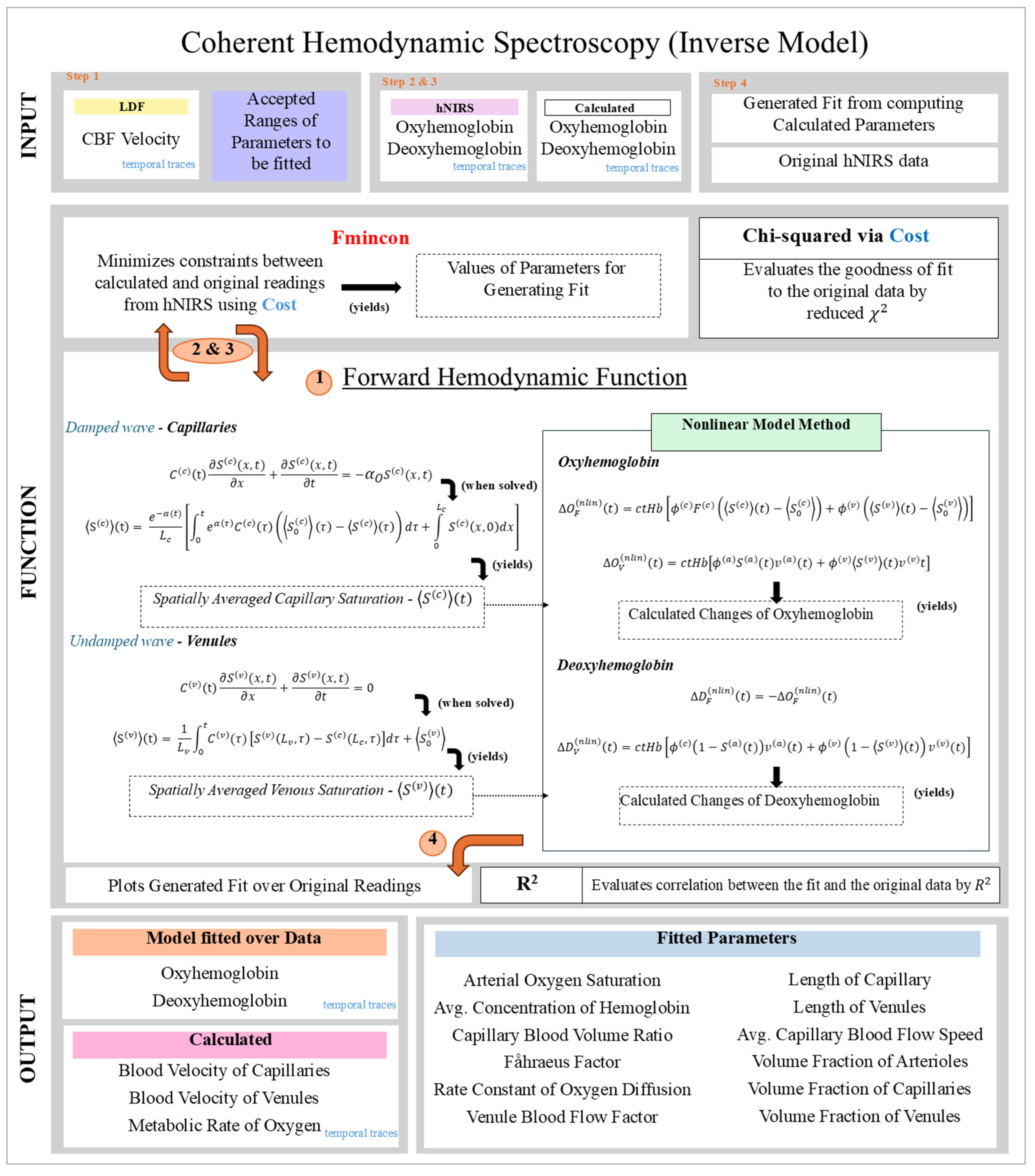
Figure 2.
Changes in the simulated and computed CHS model variables. (a): Computed [HbO2] and [HHb] responses to simulated [tHb] and CBF changes (b); (c): Computed changes in StO2 (tissue oxygen saturation); (d) Computed responses in 〈
Figure 2.
Changes in the simulated and computed CHS model variables. (a): Computed [HbO2] and [HHb] responses to simulated [tHb] and CBF changes (b); (c): Computed changes in StO2 (tissue oxygen saturation); (d) Computed responses in 〈
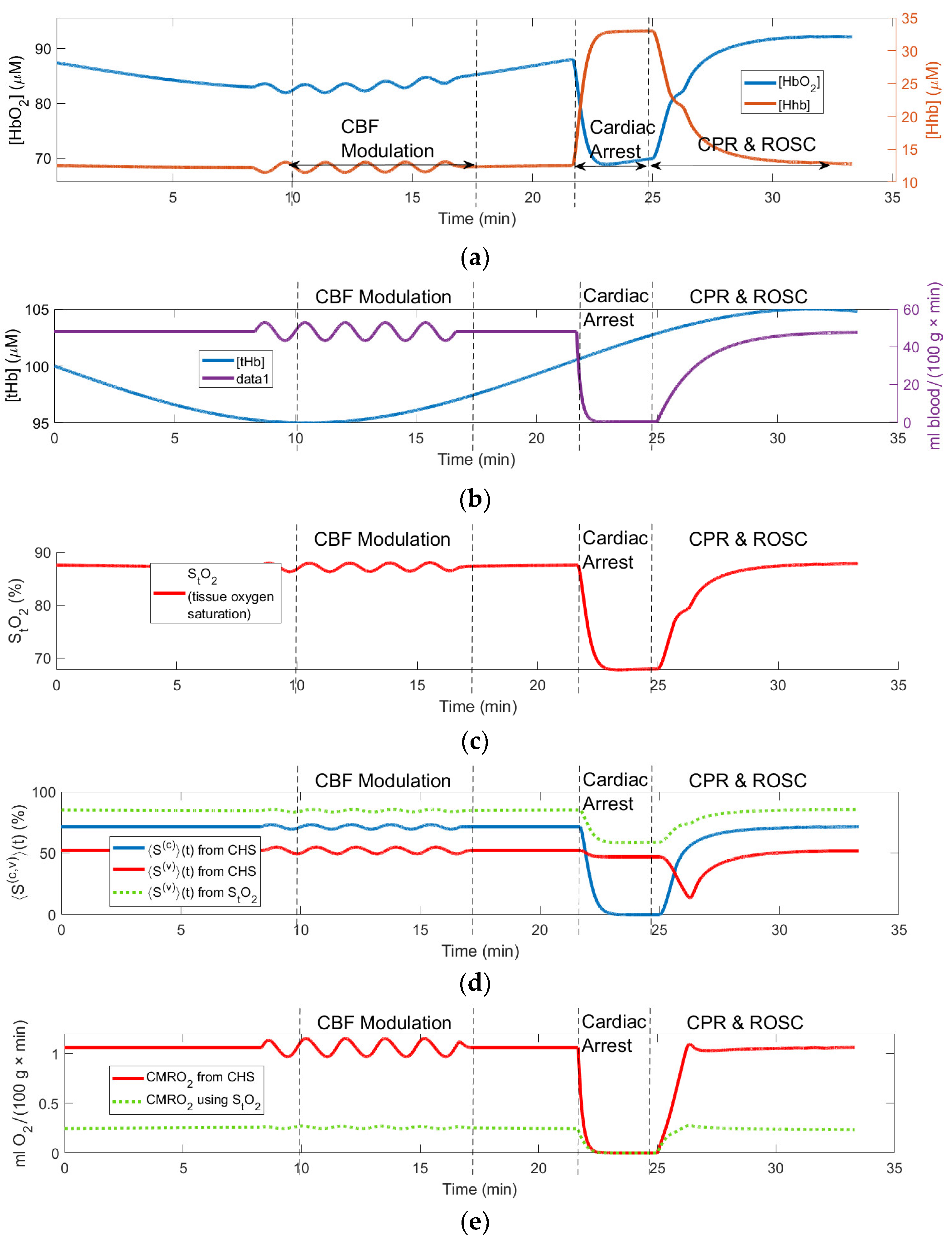
Figure 3.
Physiological variables measured and computed during a cardiac arrest experiment on a pig: (a) measured and fitted traces of [HbO2] and [HHb], R2 = 0.96; (b) measured [tHb] and computed CBF; (c) computed capillary 〈
Figure 3.
Physiological variables measured and computed during a cardiac arrest experiment on a pig: (a) measured and fitted traces of [HbO2] and [HHb], R2 = 0.96; (b) measured [tHb] and computed CBF; (c) computed capillary 〈
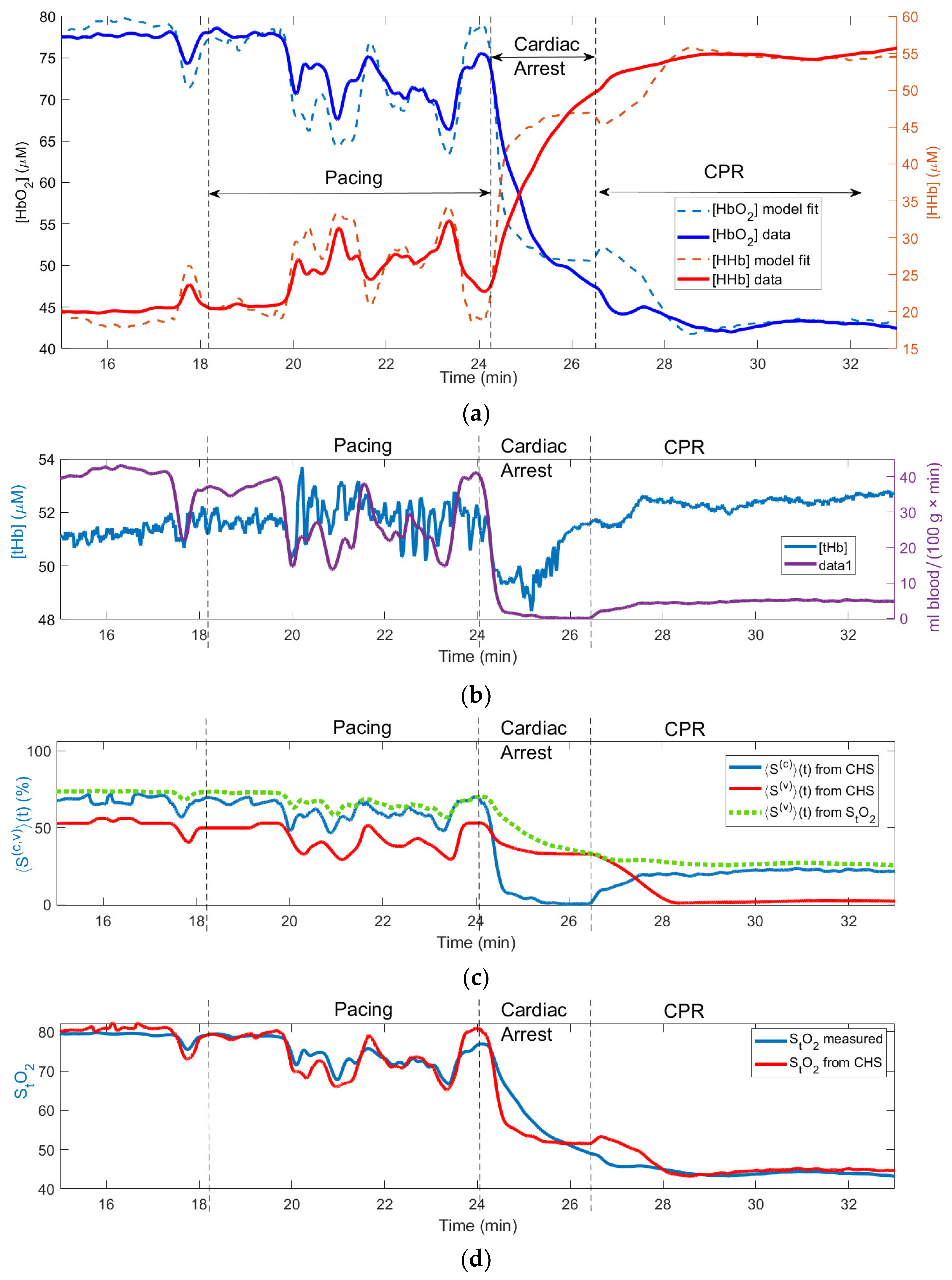
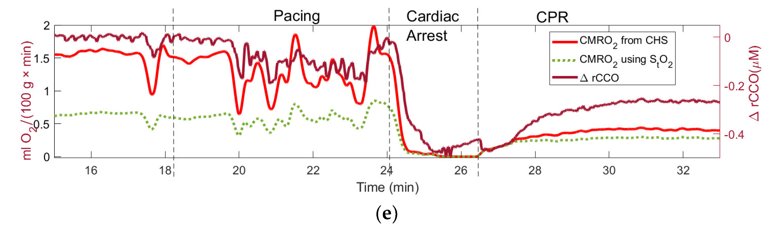
Figure 4.
Variables and parameters during a cardiac arrest experiment on a pig obtained using sweeping 30-second interval fitting: (a) measured and fitted traces of [HbO2] and [HHb], R2 = 0.99; (b) recovered changes in arterial oxygen saturation
Figure 4.
Variables and parameters during a cardiac arrest experiment on a pig obtained using sweeping 30-second interval fitting: (a) measured and fitted traces of [HbO2] and [HHb], R2 = 0.99; (b) recovered changes in arterial oxygen saturation
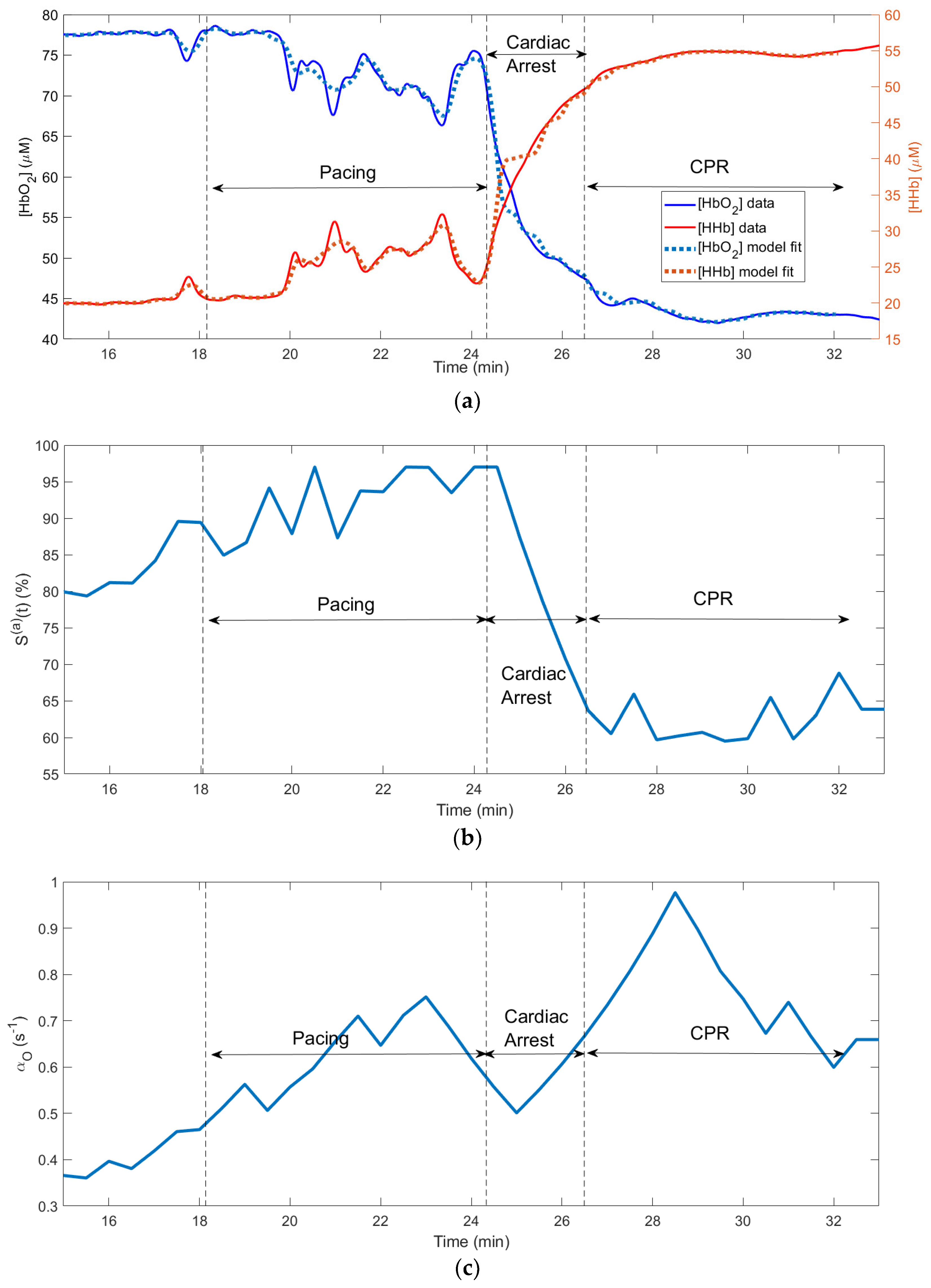
Table 1.
Fitted parameters used in the non-linear CHS model with their definitions, units and ranges of their values.
Table 1.
Fitted parameters used in the non-linear CHS model with their definitions, units and ranges of their values.
| Fitted parameter | Definition | Unit | Value Range |
|---|---|---|---|
| Arterial oxygen saturation | % | 80-99 | |
| ctHB | Hemoglobin concentration in blood | mM | 2-2.6 |
| Capillary baseline blood volume ratio | - | 0.2-0.8 | |
| Fåhraeus factor | - | 0.6-0.9 | |
| Rate of oxygen diffusion | s-1 | 0.6-1 | |
| Capillary length | mm | 0.4-0.8 | |
| Venule length | mm | 0.5-1.2 | |
| cBFf | Capillary Blood flow factor | mm/s | 0.6-1 |
| vBFf | Venule Blood flow factor | mm/s | 0.1-1 |
| Arterioles volume fraction | - | 0.001-0.05 | |
| Capillary volume fraction | - | 0.005-0.05 | |
| Venules volume fraction | - | 0.001-0.05 |
Table 2.
Values of the model parameters: normal baseline ranges from literature [1], values used for simulating changes shown in Figure 2, and values obtained by applying the inverse algorithm to the animal data (see Figure 3).
| Fitted parameter | Normal baseline ranges | Used for simulation (Figure 2) | Obtained by fitting (Figure 3) |
|---|---|---|---|
| (t) | 60-99 % | 95 % | 85 % |
| ctHB | 2.0 – 2.6 mM | 2.3 mM | 2.2 mM |
| 0.2 – 0.8 | 0.50 | 0.56 | |
| 0.6 – 0.9 | 0.80 | 0.41 | |
| 0.6 – 1.0 s-1 | 0.80 s-1 | 0.60 s-1 | |
| 0.1 – 0.7 | 0.60 | 0.15 | |
| 0.4 – 0.8 mm | 0.60 mm | 0.56 mm | |
| 0.5 – 1.2 mm | 1.00 mm | 1.17 mm | |
| cBFf | 0.6 – 1.0 mm/s | 0.00 – 1.00 mm/s | 0.99 mm/s |
| vBFf | 0.1-1.0 mm/s | 0.00 – 1.00 mm/s | 0.56 mm/s |
| 0.001 – 0.050 | 0.03 | 0.013 | |
| 0.005 – 0.050 | 0.0150 | 0.032 | |
| 0.001-0.050 | 0.005 | 0.019 |
Disclaimer/Publisher’s Note: The statements, opinions and data contained in all publications are solely those of the individual author(s) and contributor(s) and not of MDPI and/or the editor(s). MDPI and/or the editor(s) disclaim responsibility for any injury to people or property resulting from any ideas, methods, instructions or products referred to in the content. |
© 2025 by the authors. Licensee MDPI, Basel, Switzerland. This article is an open access article distributed under the terms and conditions of the Creative Commons Attribution (CC BY) license (http://creativecommons.org/licenses/by/4.0/).
Copyright: This open access article is published under a Creative Commons CC BY 4.0 license, which permit the free download, distribution, and reuse, provided that the author and preprint are cited in any reuse.


