Introduction to Geospatial Analysis for Business Analytics

1. INTRODUCTION TO GEOSPATIAL ANALYSIS

Geospatial analysis involves collecting, combining, visualizing and modeling various types of geospatial data. It is used to model and represent how people and phenomena interact within space, as well as to make predictions based on trends in the relationships between people and places. Specifically, we will focus on the visualization and modeling of spatial data, leaving aside the section of extraction and manipulation of geographic data, which would be a separate paper.

Some benefits of using geospatial data in analytics are the following. First, identifying spatial patterns and trends. Some relationships cannot be understood without knowing “where” (or “when”) they are occurring. Second, more opportunities for segmentation: when geographical location is added as a specific variable, you can segment and filter based on geography, which makes your entire analysis more detailed. Third, modeling the real world, because everything has an (X,Y) geographical position, so analysis without location is already missing a key component. Forth, accurate predictions lead to better decision-making. When you study a phenomenon over time in the context of particular locations, this helps you better predict not only what will happen, but also where it will happen.

Additionally, it should not be a surprise that geospatial data is increasingly being integrated into several different industries and corporate functions, because it provides a lot of extra information and context that most other types of data do not (SAFEGRAPH 2024a,b). Although geospatial analysis is widely used across various industries and professions, here are some of the most popular professions that use geospatial analysis in the area of economics and business administration:

A)

In the private sector: Market researchers and independent consultants, retailers, telecommunication and network companies, transport and logistic companies, investment banks and private equity firms, insurance companies, and property appraisers.

B)

In the public sector and government: Academic research, national banks (e.g. Bank of Spain), urban and regional planners, real estate developers, state security forces and criminologists.

Hence, geospatial data and methods are used in scientific or governmental administration contexts, but it has an increasing number of commercial uses as well. Next, we present 10 scenarios where you can make use of geospatial analysis:

• Mapping. A good example of geospatial data use is visualizing the area that the data describes, like transportation routes, building sites, administrative areas, etc. A precisely drawn map can be an immensely powerful tool. This is the case of travelers who may not know their way around a particular area and need to use Google Maps or Waze, among others.
• Site selection There are some things to consider when selecting or deselecting retail sites: Where locations are currently located? Are other nearby stores in competence (market competition), or possibly collaboration (market agglomeration)? How close is a shop to where the target customers live? How accessible are the company sites to those target customers? Where are the successful stores whose qualities should be mimic?
• Visit attribution. Another use case is telling the difference between someone entering your store or just simply passing by. You can compare accurate building area data with precise GPS from mobile devices to know how many people entered your store.
• Urban planning. If you are working in the government or the public sector, you can make sound planning decisions based on data about building location, people living areas, commuting flows, traffic data, etc. For instance, you can plan construction for roads or other transportation systems to reduce walk/drive times work and/or education facilities. Or, on the contrary you can plan to build hospitals or schools in areas with good access.
• Network planning. For example, foot traffic data can help providers, like Movistar, Orange, etc. They can implement a sufficient coverage with the least amount of hardware. They also can fix the price they charge for WIFI hotspots, with installations in higher-traffic areas being more expensive. For other businesses, like retailers, they can decide on the telecom plan and infrastructure they need.
• Investment research. Investment banks and private equity firms can model and predict consumer behavior and movement patterns using variables like location data for stores, and other points of interest, traffic data, and contextual data (like per capita income, population by age, etc.). This will allow them to get a better picture of how the businesses they are investing in are actually performing or the ones they are planning on investing in.
• Competitive intelligence. Competition affects in part a business performance. For instance: A map can reveal customers’ choice among different competitors depending on parking space and transportation routes. It is also possible to discover if a business stores are too close together in terms of walk/drive time, and if they are competing over the same customers (they are being phagocytized). Or it can also be noticed if nearby stores that are assumed to compete each other, actually are not, because the target customers may be coming from different locations.
• Risk assessment. The insurance industry is another sector that is making use of geospatial analysis. For instance, to assess building vulnerability to things like destructive weather, foods, fire, vehicle accident, etc., insurers need to know a number of their geospatial attributes like where a building is, how much space it takes up, how close it is to surrounding buildings, how many businesses are contained in the same building, what they do or sell, since some businesses present more hazards than others. Regarding occupancy, the more people living in or visiting a building daily, the greater the risk for an accident to happen.
• Trade area analysis: Sometimes it is not enough to just look at how accessible a location is and how close competitors are. It must be known, for example: if potential customers’ lifestyles make them want to buy what you are selling, if they would afford the products a business is selling, based on their average income range, if there are many competitors nearby and how well-established they are, if the competitors have a good reputation, to consider another area where compete with easiest rival businesses, etc. Asking these types of questions helps you more accurately adjust your site selection (among other things) to satisfy the people who will most likely be your clients.
• Consumer insights. A specific geospatial data sample may be able to give you even more granular insights into your customers’ shopping habits. For instance, looking at establishments that consumers visit before or after they come a specific shop. This could be the case of a health-conscious shop or restaurant noticing that a lot of customers are going to gyms or yoga studios before or after they go to their shop or restaurant. Hence, this knowledge could be used to identify nearby stores of this type on a map and approach them for cross-promotion opportunities.

In this paper, an introduction to some of the practical issues necessary to get into geospatial analysis applied to business analytics is given. After a first chapter dedicated to present the characteristics of spatial data, the following chapter shows some web portals with important resources for working with spatial data (basically, geocoding of addresses, digital maps in different formats and map viewers). Finally, important servers with maps and software useful for the analysis of spatial data applied to the company will be presented. The Conclusion section, References and Appendix close.

2. WHY IS SPATIAL DATA SPECIAL?

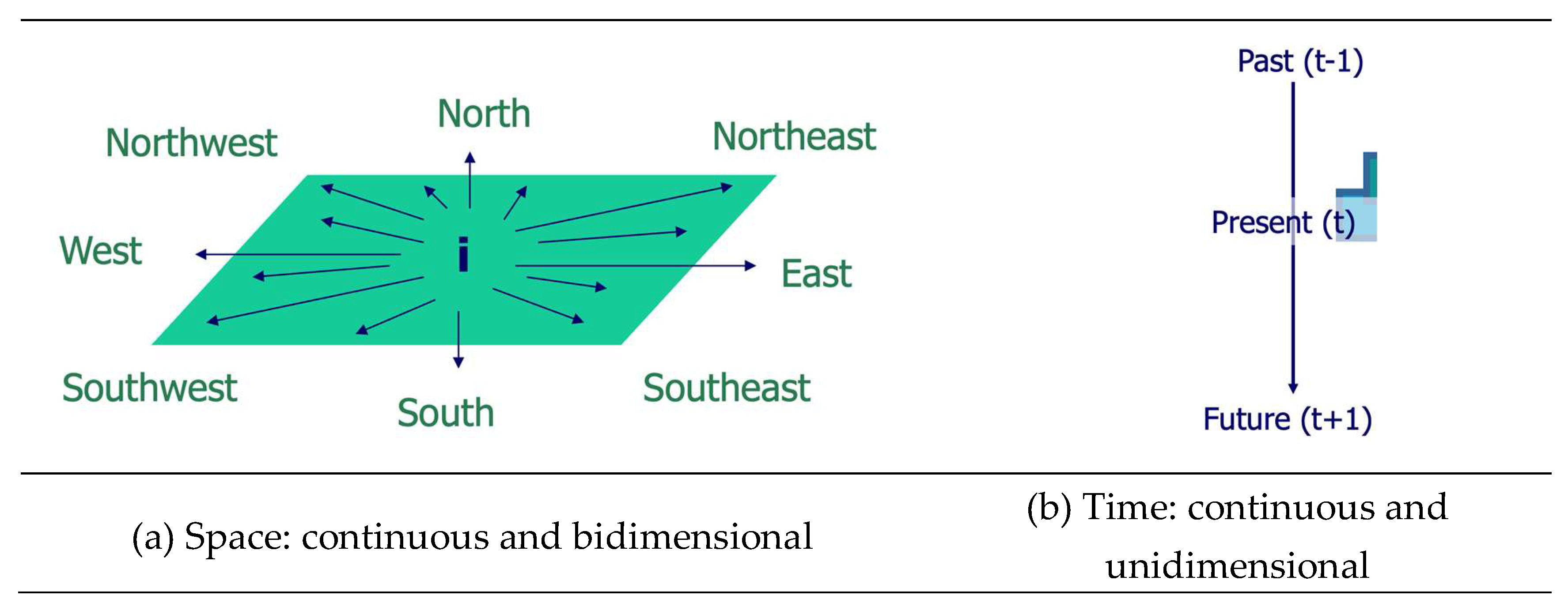
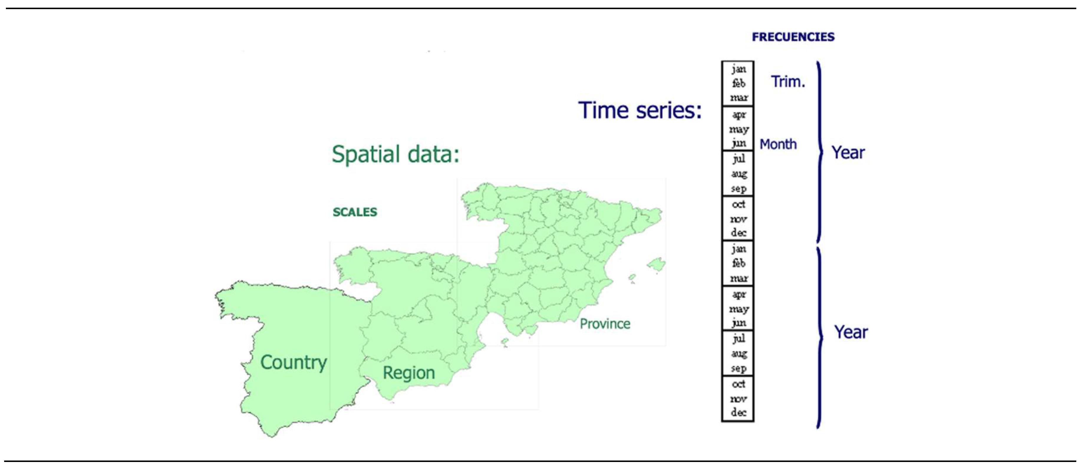
2.1. SPATIAL DIMENSIONS

The nature of spatial data is “special”, different and more complex than, for example, the nature of time series (Figure 1). They are cross-sectional data with the following characteristics (Chasco and Fernández-Avilés 2009):

-

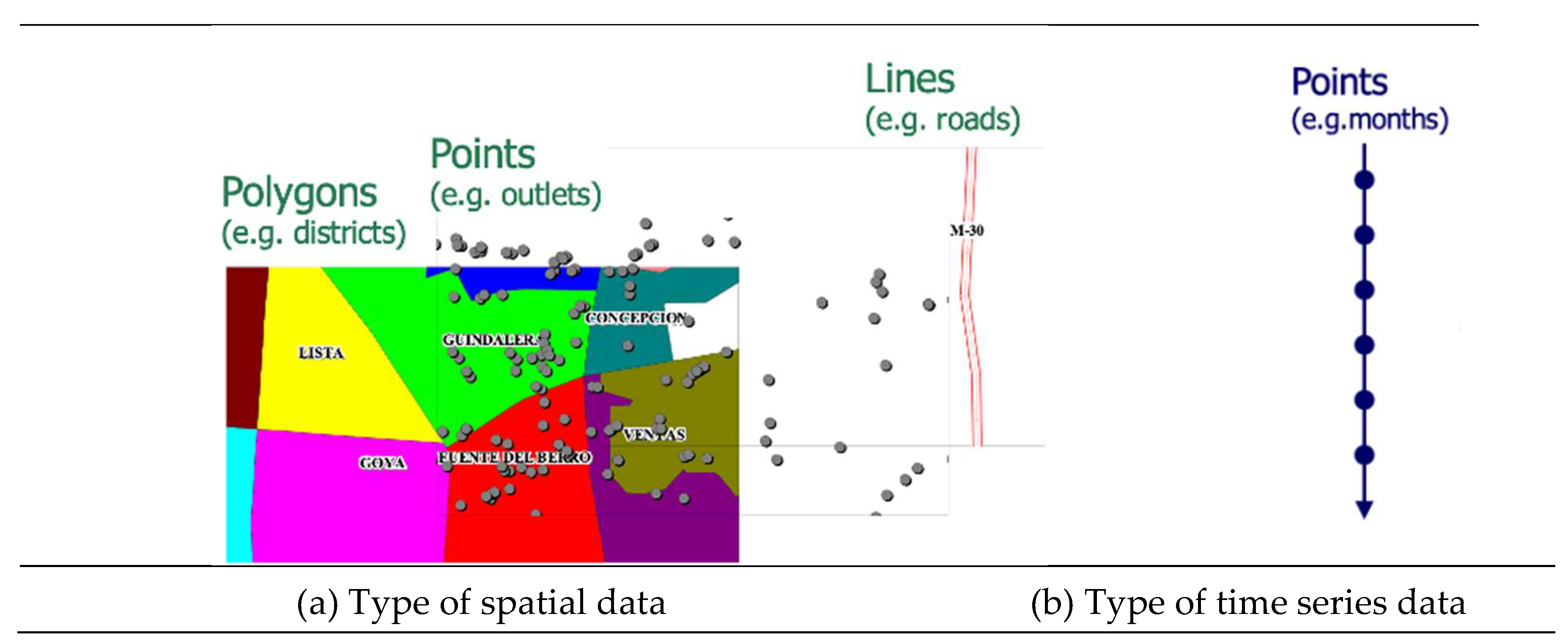
Space can be represented as a continuous, two-dimensional surface, while time is represented as a continuous, one-dimensional line.

-

In geographic space, any point “i” is interconnected with the other points in a 360-degree circular space., usually simplified by the 4 cardinal points (north, south, east and west) and intercardinal points (NE, SE, NW, SW). In time, a moment “t” is related linearly in 2 directions: to the past (“t – 1”) and to the future (“t + 1”).

-

In geographic space, any point “i” is interconnected with the other points in a 360-degree circular space., usually simplified by the 4 cardinal points (north, south, east and west) and intercardinal points (NE, SE, NW, SW). In time, a moment “t” is related linearly in 2 directions: to the past (“t – 1”) and to the future (“t + 1”).

2.2. SPATIAL SCALES

Although time and geographic space are both continuous in nature, they can be artificially discretized into frequencies and scales, respectively. This allows the elaboration of statistics, which will be referred to these discretizations (Figure 2).

In the case of time series, time is divided into years, semesters, quarters, months, weeks, and so on. As for geographic space, its division is more complex because there are no clear international agreements in this regard. For example, the division of the World into countries is usually more or less well accepted, except in situations of discord (such as the state of Palestine or Taiwan, recognized by some and rejected by others). However, on the intra-national divisions, each country has its own divisions according to its own (historical or economic) criteria.

A special case is the European Union (EU), which has created a supranational territorial division (Wikipedia 2024a, Eurostat 2024a,b,c). Specifically, Eurostat, its statistics office, recognizes the following divisions and sub-divisions:

1)

Member countries.

2)

NUTS 1: major socio-economic regions.

3)

NUTS 2: basic regions, which are eligible for the EU regional policies.

4)

NUTS 3: small regions.

5)

LAU: municipalities or communes.

The acronym NUTS means Nomenclature of Territorial Units for Statistics and LAU is Local Administrative Units.

-

The NUTS are the reference countries’ regions, which have been developed for statistical purposes and, in the case of the NUTS 2, to frame EU regional policies. Based on existing national administrative subdivisions, they have been established following criteria based on population segments (with some exceptions).

-

The LAUs are a subdivision of the NUTS 3 regions covering the EU's whole economic territory. They are appropriate for implementing local level typologies like the one that classifies LAUs as cities (densely populated areas, towns and suburbs (intermediate density areas) and rural areas (thinly populated areas).

For example, in the case of the member country of Spain, the territorial divisions are the following:

1)

7 NUTS 1: Noroeste, Noreste, Comunidad de Madrid, Centro, Este, Sur, and Canarias (their official name is in Spanish).

2)

19 NUTS 2: the 17 autonomous communities and 2 autonomous cities (Ciudad de Ceuta and Ciudad de Melilla).

3)

59 NUTS 3: the 50 provinces, 3 Balearic Islands (Mallorca, Menorca, and Eivissa and Formentera), 7 Canary Islands (Gran Canaria, Tenerife, Lanzarote, Fuerteventura, La Palma, La Gomera and El Hierro), plus Ceuta and Melilla.

4)

8,131 LAU: the municipalities.

Below the municipal organization it is quite common in many countries for census tracts to exist, as the minimum level of administrative territorial subdivision for which statistics are compiled. In Spain, municipalities are first divided into districts and these into census tracts. Some large cities, such as Madrid and Barcelona, also contemplate the division of districts into neighborhoods and these into census sections. For example, the municipality or city of Madrid consists of 21 districts, 131 neighborhoods and 2,398 census tracts.

Finally, in addition to administrative divisions, the EU provides basic data (such as population) for other types of divisions for its territory. For example:

a)

Postal code areas: territorial divisions that are important to companies because it is a piece of information that customers tend to provide in surveys and loyalty cards without much suspicion. However, these divisions do not coincide with the administrative divisions of NUTS and LAUs, for which the statistical institutes produce most of their databases. Eurostat has therefore developed the TERCET NUTS-postal codes matching tables containing a lookup-list of European postal codes and their corresponding NUTS codes.

b)

Square grids of small resolution (1x1 and 10x10 km). In this case, administrative divisions (such as countries) are not respected. For example, there are 1x1 grids that include territory of Irun (Spain) and territory of Hendaye (France). In this case, there are areas that are not gridded because there is no population in them (such as large areas of the Pyrenees).

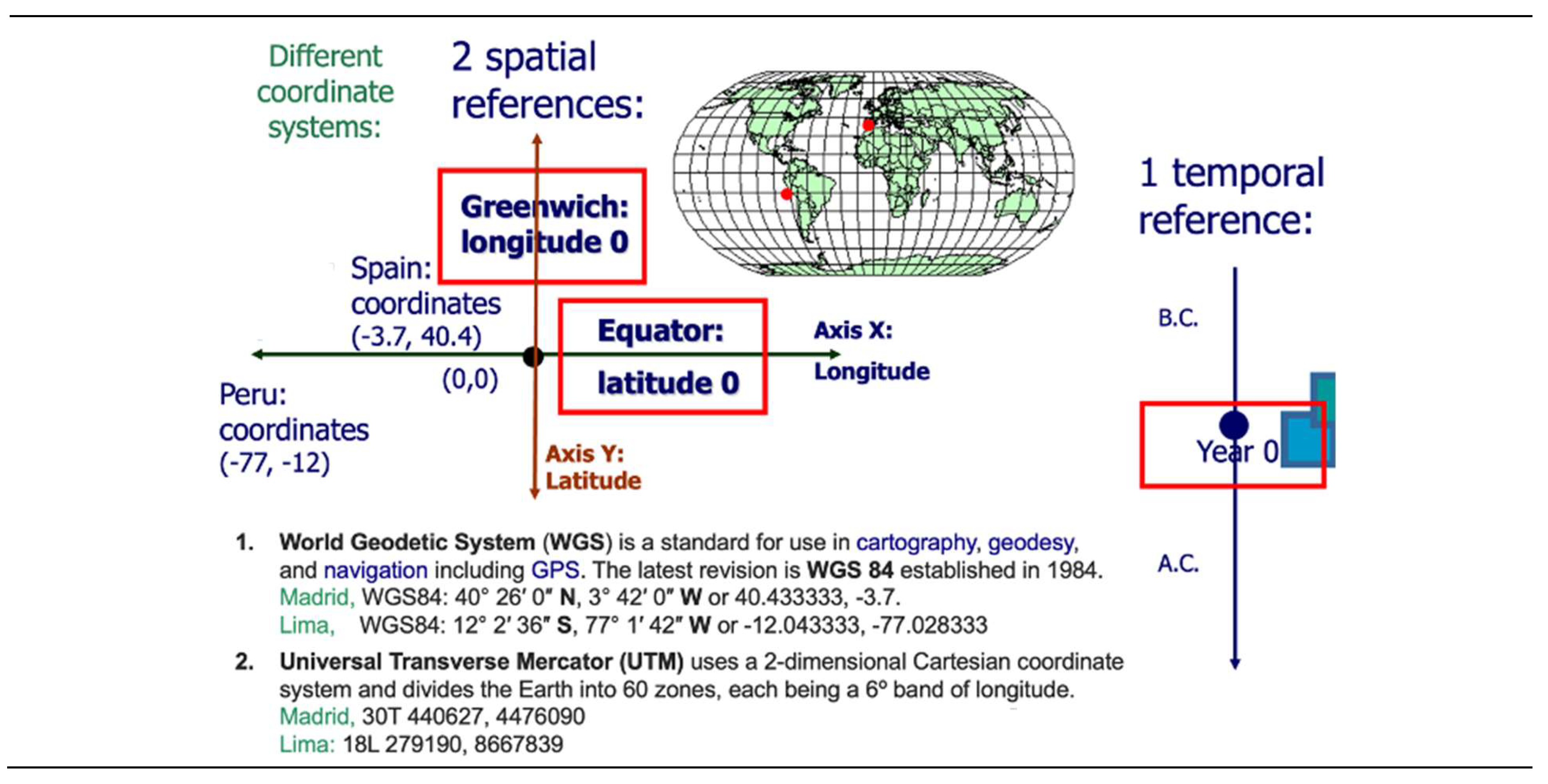
2.3. SPATIAL REFERENCES

Another difference between geographic space and time is that space has many referencing systems, while time -except in non-Christian culture countries- has only one: year 0, corresponding to the birth of Jesus Christ. Therefore, it is a referential point in a linear system, which count years and centuries as before and after Christ.

On their side, spatial observations need to be georeferenced in a two-dimensional Cartesian coordinate system (Figure 3). However, the Earth is not flat but a near-spherical surface, what requires a transformation (Chasco and Fernández-Avilés 2009; Anselin 2023).

2.3.1. Transformation from a spherical shape to a flat map

The basis for this transformation is latitude and longitude coordinates (i.e., vertical and horizontal dimensions, respectively), which are measured in degrees. They situate each location with respect to the equator (X axis) and the Greenwich Meridian, which is a location near London, UK (Y axis). For example, the municipality of Madrid is west of Greenwich (negative longitude) and north of the equator (positive latitude), while South Africa is east of Greenwich (positive longitude) and south of the equator (negative latitude).

In order to give a location a latitude and longitude, two steps are necessary:

1)

Selecting a so-called geodetic datum model. The most commonly used datum is the World Geodetic System of 1984, WGS 84, which represents the Earth as an ellipsoid (and not as a perfect sphere). In Europe, an alternative is the European Terrestrial Reference System 1989, ETRS89.

2)

Converting the latitude-longitude coordinates to cartesian X-Y coordinates in a planar system, using a cartographic projection. Hundreds of projections have been developed, as mathematical methods of converting a 3-dimensional quasi-sphere to a 2-dimensional flat map. The use of an inappropriate projection may yield to misleading distance computations among locations, especially for analyses that cover large areas (e.g., continent-wide).

Spatial coordinates are projected when they are expressed in distance units of meters or feets, and they are unprojected when they are expressed in decimal degrees (not in distance metrics). Hence, using the latitude-longitude decimal degrees coordinates to compute the distance between two Earth points is not incorrect because they are expressed in degrees or angles, not in proper distance units. The calculation of Euclidean distance for two spatial locations is only possible for projected coordinates.

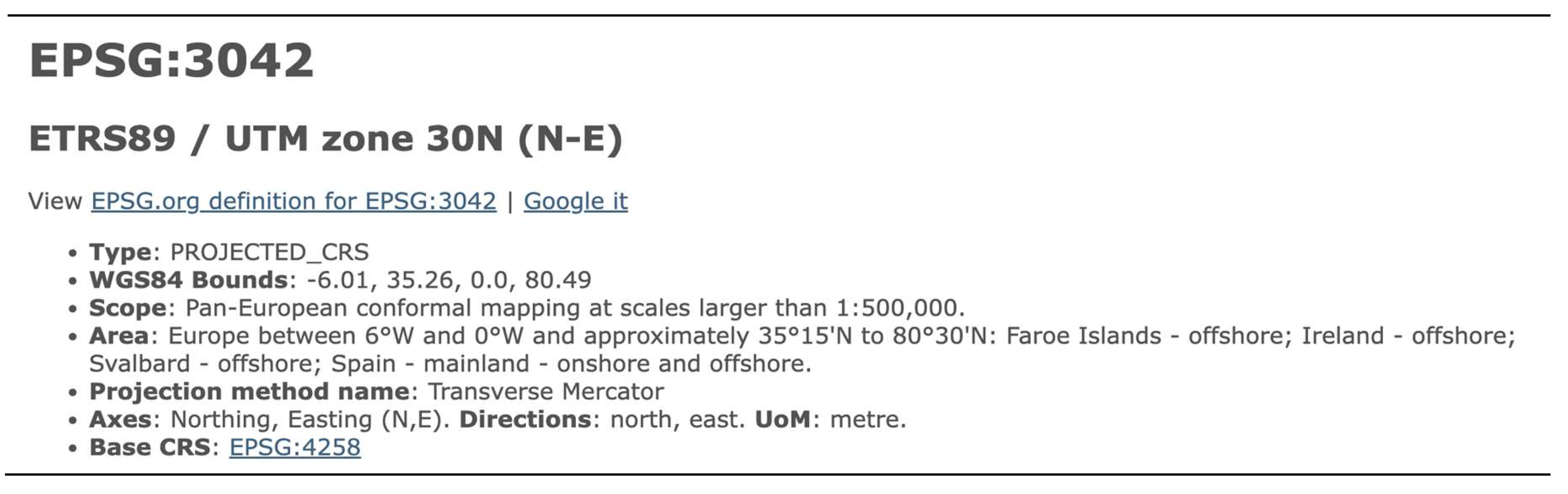
2.3.2. Coordinate Reference System (CRS)

A CRS is a formal representation of location that contains information about the geodetic datum model and the cartographic projection, joint to some other data. It is also identified with a code, such as the developed by the European Petroleum Survey Group (EPSG). The web site spatialreference.org contains hundreds of projection definitions including the CRS information for all of them.

The latitude-longitude decimal degree non-projected coordinates are also included in this web site to allow for transformation to projected coordinates using a suitable software, as will be seen later. Curiously, it is referred to as “geographic projection” (even though strictly speaking no projection is involved) and with a datum code “EPSG 4326”.

If a digital map is expressed in X-Y decimal degrees, it should include its CRS which can be expressed as:

+proj=longlat +ellps=WGS84 +datum=WGS84 +no_defs

2.3.3. Selection of a projection

As already said, it is preferred to use projected coordinates so that Euclidean distance operations and area calculations are straightforward to perform. For North America and Europe, a useful projection is Universal Transverse Mercator (UTM). The countries are divided into parallel zones, with each zone corresponds a specific projection that is represented by a CRS. For example, Spain is located in the UTM zone 30 North (there is a 30 equivalent in the southern hemisphere) while Belgium is in the UTM zone 31 North.

The web site spatialreference.org provides a CRS which is suitable for Spain, with the following information (Figure 4):

-

CRS code: EPGS 3042

-

Geodetic datum: ETRS89

-

Projection: UTM zone 30N

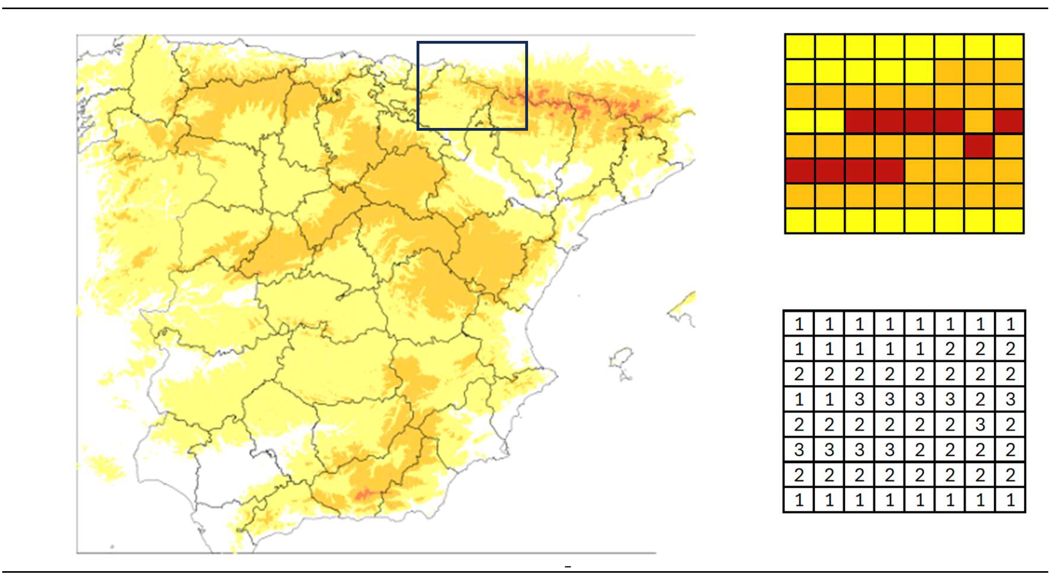
2.3.4. Types of spatial data

The two primary types of spatial data are vector and raster data. Vector data is also called “object view” versus “field view” that is the way raster data is known (Chasco and Fernández-Avilés 2009; GISGeography 2024).

a)

Raster data is made up of pixels or grid cells. They are usually small squares of equal size. Each pixel value has a value, which is represented with a color (red, green, blue, etc.). Raster data are useful for storing data that varies continuously like elevation surfaces, temperature, rainfall and contamination (Figure 5).

b)

Vector data: Vector data is not made up of a grid of pixels. Instead, vector graphics are comprised of vertices and paths. The three basic symbol types for vector data are points, lines, and polygons or areas (Figure 6).

-

Vector points are latitude-longitude (non-projected) or cartesian (projected) XY coordinates. They are useful to represent locations like houses, trees, or cities. The thickness of the dots usually represents data values (e.g., a large city will be represented by a larger diameter dot than a small town).

-

Vector lines connect the points with lines. When you connect the points in a set order, it becomes a vector line or path with each dot representing a vertex. Lines usually represent features that are linear in nature or can be built with small lines (like curves), for example, rivers, roads, and pipelines. The size of the different lines usually represents data values, like traffic (e.g., busier highways have thicker lines than abandoned roads).

-

Vector polygons join a set of vertices in a particular order and close it. Hence, in a polygon feature, the first and last coordinate pairs are the same. Vector polygons are used to show areas surrounded by boundaries like countries, regions, or grids. Data values are represented by different colors or a gradation of colors (e.g., highest values have higher values have more intense or darker colors).

3. WEB RESOURCES FOR SPATIAL DATA

3.1. GEOCODING POSTAL ADDRESSES

Geocoding is the process of converting postal addresses (such as a street address) into geographic coordinates (latitude and longitude) that can be used to create digital maps with special software called Geographic Information Systems (GIS). In addition, reverse geocoding is possible. It consists of obtaining postal addresses from coordinates. There are applications that allow geocoding addresses with some limited free version.

Sometimes the available addresses are ambiguous because they contain incorrect formatting, incomplete addresses or misspellings. In these cases, one should opt for the paid options of these web pages that contain special services designed to display several possible options and allow the user to choose them. However, there are quite good options on the web to geocode addresses.

3.1.1. Google Maps Platform

API Geocoding such that you pay for what you order (Google Maps Platform 2024).

3.1.2. ESRI’s ArcGIS Location Platform

ArcGIS Pro featured API, such that you pay for what you order (ESRI Developer 2024).

3.1.3. Precisely’s Geo Addressing

It is one of the programs included in the Precisely Data Integrity Suite, which can be bought individually (Precisely 2024a).

3.1.4. batchgeo.com

batchgeo.com is an interactive webpage which geocodes postal addresses from an Excel sheet with the following columns: Country, Address, City, State, Postcode (Batchgeo LLC 2024). It allows creating maps and exporting KML files with the Earth coordinates, which can be opened and edited from Excel to be visualized in a GIS (Figure 7). The Pro (paid) version allows faster geocoding, password protection, up to 10 users, PDF support and much more.

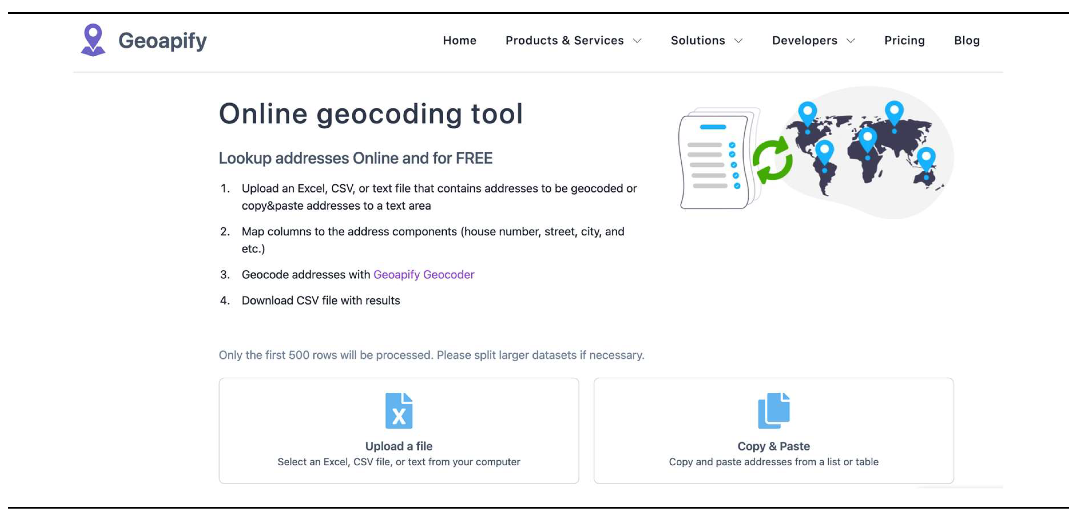
3.1.5. geoapify.com

geoapify.com is an interactive webpage which geocodes postal addresses from an Excel sheet with the following columns: house number, street, city, and etc. (Geoapify 2024). It allows geocoding addresses from XLSX, CSV, TXT files or just copy and paste addresses from a table or list (Figure 8).

The result table is downloaded in a CSV file. It contains the following elements:

a)

Original addresses.

b)

Found addresses.

c)

Their latitude and longitude coordinates.

d)

Their address components.

e)

A confidence coefficient, which indicates how confident they are in found address: a confidence equal to 1 tells that they are sure that the address is correct.

There are paid pricing plans allowing more than 3,000 credits/day, commercial use, faster geocoding (up to 5 requests/second), email and priority support, and much more.

3.2. DIGITAL MAPS FORMATS

Historically, a wide range of different formats have been developed for GIS data or digital maps, both proprietary as well as open source (Anselin 2023). The most commonly used formats are shown here. See in Appendix 1 a summary of the main characteristics of the presented digital map formats.

3.2.1. Proprietary digital maps

a)

Shapefile: the GIS vendor ESRI ("Environmental Systems Research Institute") developed the shapefile format for its ArcGIS products. The terminology is a bit confusing, since there is no such thing as one shape file, but a collection of three (or four) files:

-

The map’s main file, with the extension *.shp, is a table which each record describes a shape with a list of its vertices.

-

An index file, with the extension *.shx, which links geometry (“shp” file) with attributes (“dbf” file) based on a number.

-

A dBase table, with the extension *.dbf, which contains the spatial features attributes with one record per feature. Attribute records in this file must be in the same order as records in the main “shp” file.

-

A *.prj file with the map projection information.

The first three files (*.shp, *.shx, *.dbf) are required and the fourth (*.prj) is optional, but highly recommended. The files should all be in the same directory and have the same file name, except for the file extension.

Shapefiles are fundamentally row oriented, with each row representing a geometric shape and its associated attributes stored in columns (Table 1). The shapefiles are older structures and have a significant size limitation, up to 2 GB. It supports only vector data (point, line and polygon geometry types). ESRI has its own native raster data called Esri grid (*.adf).

b)

TAB: The GIS vendor Precisely develops the TAB file format for its MapInfo software products (Precisely 2024b). Again, these maps are a collection several files, which are related with two basic environments for working in MapInfo: the "Browser View" (*.TAB, *.DAT) and the "Mapper View" (*.MAP, *.ID, *.IND).

TAB files are also row oriented. They have a size limitation, around 2 GB, though they depend on the MapInfo version and the computer capacity. It supports only vector data (point, line and polygon geometry types). MapInfo has its own native raster data called Multi-Resolution Raster, MRR (*.mrr).

c)

File Geodatabase (*.gdb): It is an ESRI’s data container, which is row-oriented, allowing the efficient storage and management of large amounts of geospatial data within a single file by using compression to minimize space. It supports vector and raster data and can store up to 1 TB of data per file (Wikipedia 2024b).

3.2.2. Open-source digital maps

In the open-source world, there are different formats for digital maps:

a)

GeoArrow (*.arrow): It allows storing geospatial data in Apache Arrow and Arrow-compatible data structures and formats, which is specified as a columnar memory format (Table 1) and is supported by many programming languages and data libraries (GeoArrow 2024). Spatial information can be represented as a collection of discrete objects using points, lines and polygons (i.e., vector data). It was designed to manage big databases and has no specific technical size limit beyond the limitations of the file system (e.g., in the Windows operative system, it can reach more than 200 TB).

a)

Geography Markup Language or GML (*.gml): GML of the Open Geographic Consortium (OGC) is a standard Extensive Markup Language (XML) grammar for defining geographical features (Wikipedia 2024c). Hence, it is neither a row-oriented nor a column-oriented format. It organizes data hierarchically using nested elements. It supports point, line and polygon geometry types (only vector data, not raster). It has no specific technical size limit beyond the limitations of the file system. However, since it is a text format, large files can become unmanageable.

b)

GeoJSON (*.geojson, *.json): It is an increasingly common format for open-source digital maps (Anselin 2023). It is the geographic augmentation of the JSON standard, which is derived from JavaScript Object Notation. This format is contained in a text file, and it is easy for machines to read, due to its highly structured nature in a hierarchical scheme (it is not strictly row or column oriented as other formats). It supports point, line and polygon geometry types (only vector data, not raster).

It has no specific technical size limit beyond the limitations of the file system or the environment in which it is being used. However, since it is a text format, large files can become unmanageable.

c)

GeoPackage (*.gpkg): It is a universal file format built on the basis of SQLite, for sharing and transferring vector and raster spatial data (Open Geospatial Consortium 2024). It is a single file, which has been designed to store complex and voluminous data (up to 140 TB). Since SQLite is a type of the relation SQL database, it is specified as a row-oriented data.

d)

GeoParquet (*.parquet): It is an OGC under development standard that adds interoperable geospatial types (point, line, polygon) to Parquet (Ministerio para la Transformación Digital y de la Función Pública 2024). Both Parquet and GeoParquet are defined as a column-oriented data format that is intended as a modern alternative to row-based CSV files. It was designed to manage big databases and has no specific technical size limit beyond the limitations of the Hadoop file system, which can reach several TB.

e)

Keyhole Markup Language or KML (*.kml): KML allows geographic annotation and visualization within two-dimensional maps and three-dimensional Earth browsers (Wikipedia 2024d). Since it is an XML-based format, it is neither a row-oriented nor a column-oriented format. It organizes data hierarchically using nested elements. It was developed for use with Google Earth. The KML file specifies a wide set of vector data features (images, polygons, 3D models, textual descriptions, etc.) with the exception of raster data. It has no specific technical size limit beyond the limitations of the file system. It is advisable to keep KML files under a few megabytes to ensure good performance and responsiveness.

For its reference system, KML uses 3D geographic coordinates: longitude, latitude, and altitude, in that order, with negative values for west, south, and below sea level. Altitude is expressed in meters. For example, the capital city of Spain, Madrid, has the following 3D geographic coordinates: (40.4168, -3.7038, 667).

f)

SpatiaLite (*.sqlite): SpatiaLite is an open-source library intended to extend the SQLite core to support fully fledged Spatial SQL capabilities (Wikipedia 2024c). SQLite is intrinsically simple and lightweight. As an SQLite extension, it is a row-oriented database management system. SpatiaLite primarily focuses on vector data (polygons, points, lines), although it also includes limited support for raster data through its RasterLite2 extension. SpatiaLite databases have a theoretical maximum size limit of about 140 terabytes. However, practical limits are generally much lower, depending on the operating environment.

Finally, it is important to note that a digital map can include one or more spatial layers and databases. For example, a map of a city can include only the spatial layer for zoning (e.g., districts) or other spatial layers for traffic density, public transportation routes, and population density, each of these independently analyzed with their own databases. Spatial layers can be of polygonal, point and linear types.

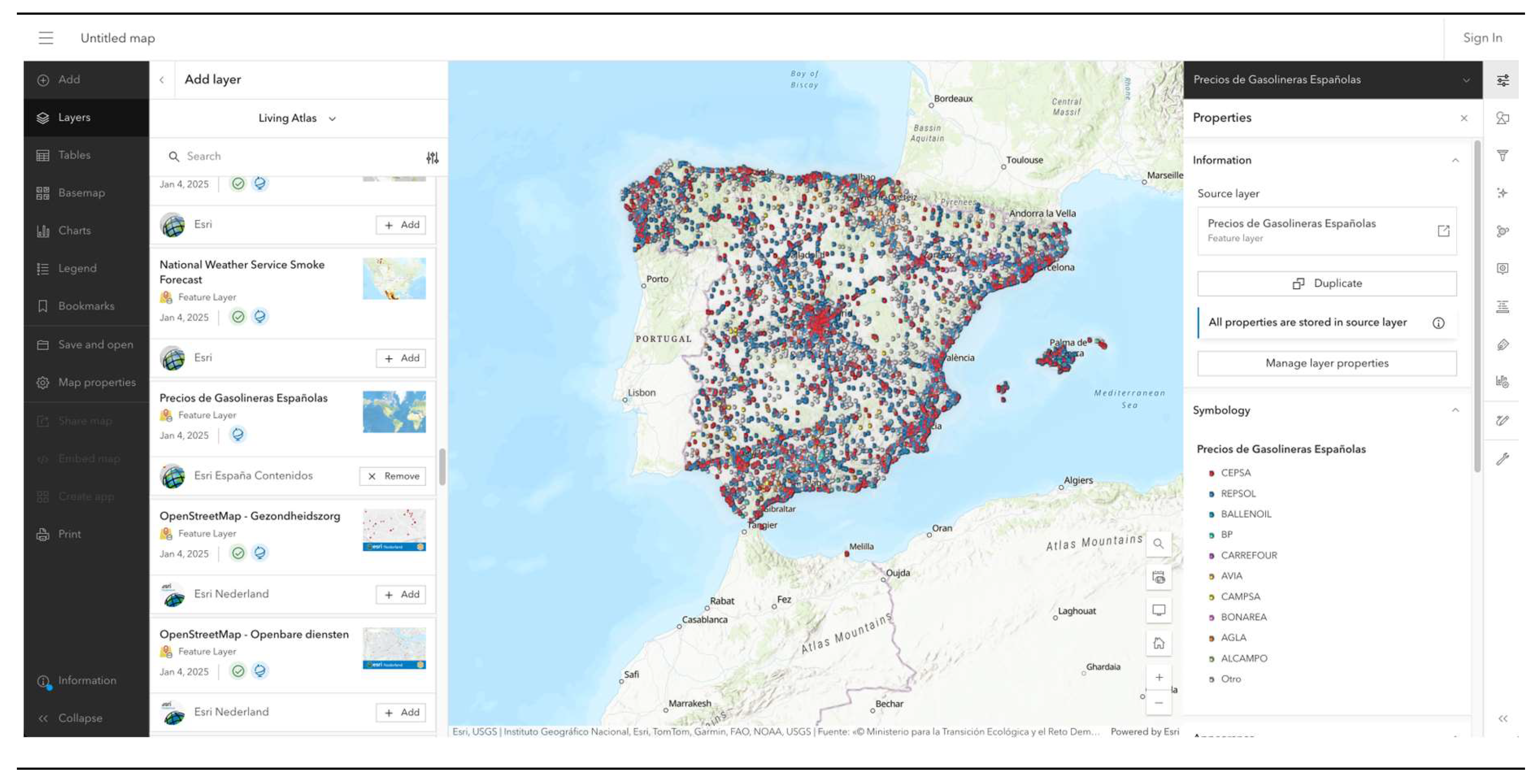
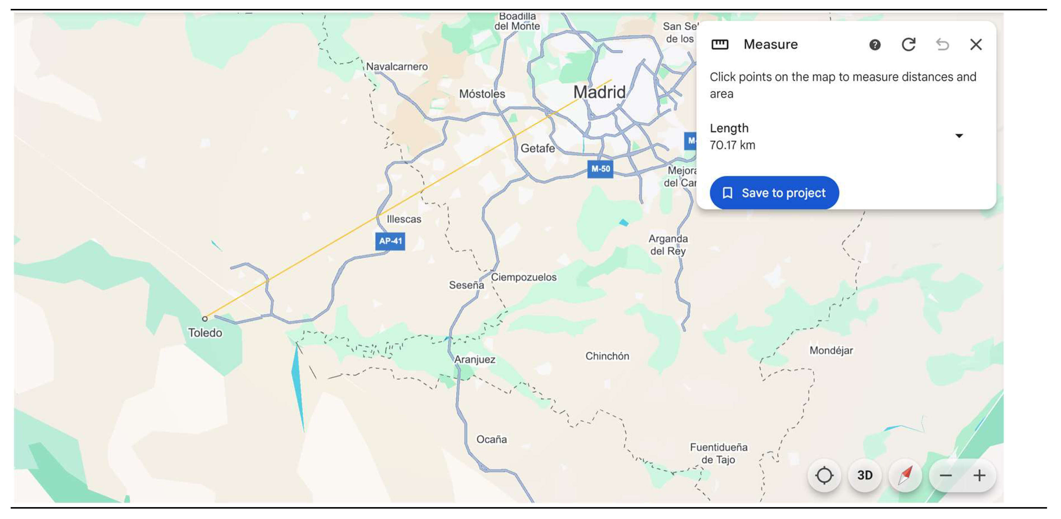
3.3. MAP VIEWERS

Currently, there are hundreds of web pages that contain digital maps: some are paid, and others offer the information for free (with or without an account creation). Here we will focus on the sites that specifically offer free map viewers. A map viewer is an online tool that allows users to view, interact with, and analyze geographic information on digital maps. Here are some basic functions of a map viewer:

-

Zoom and Pan: zoom in and out and move around the map to explore different areas.

-

Layer Control: toggle different map layers on and off, such as roads, terrain, satellite imagery, and more.

-

Search and Query: search for specific locations, addresses, or points of interest and get detailed information about them.

-

Data Visualization: visualize various types of data, such as population density, weather patterns, or traffic conditions, on the map.

-

Upload digital maps: upload own digital maps to the platform to visualize them with a more complete base map.

One of the most popular viewers for worldwide data, with free access and without the need to create an account, is “ArcGIS Living Atlas of the World” (ESRI 2025a).1 It is an open data portal that offers maps produced by ESRI itself or by collaborators. The content of this website includes maps of various locations and scales, although maps of the United States dominate, that can be opened with Map Viewer (ESRI 2025b). In addition to the visualization of one or more layers, it is possible to edit somehow the features displayed, add a data table, import maps from an external URL and export the map to a web page with its corresponding URL (Figure 3). Obviously, being a viewer, it is not possible to export the digital map, or the data included in it, except as a screenshot.

Most national, supranational (such as Eurostat) and regional statistical institutes offer one or more viewers. Sometimes, they are located on a page whose access is clearly indicated, but other times, it is difficult to locate the geographical data viewers within a statistical website. Moreover, geo-viewers have also become fashionable in the press, blogs, social networks, etc.

Figure 3. Map from ArcGIS Living Atlas of the World represented in Map Viewer.

Figure 3. Map from ArcGIS Living Atlas of the World represented in Map Viewer.

4. DIGITAL MAP SERVERS AND SOFTWARE FOR SPATIAL DATA

4.1. WEB PAGES WITH FREE DIGITAL MAPS

Digital maps can be purchased from specialized companies, but they can also be downloaded, in various formats and qualities, from certain web servers for free. However, this was not always the case, since the production of digital maps was expensive, and the smaller the geographic scale of the map, the higher the cost of acquiring them. Here we present some web pages that are relevant for their international and national coverage of Spain.

4.1.1. OpenStreetMap, OSM (OpenStreetMap Foundation 2025)

OpenStreetMap provides map data for thousands of websites, mobile apps, and hardware devices. It is built by a community of mappers (engineers, GIS professionals, etc.) that contribute and maintain data about roads, trails, cafés, railway stations, and much more, all over the world. OpenStreetMap is open data: you are free to use it for any purpose as long as you credit OpenStreetMap and its contributors. The main problem with the maps exported by OSM is that they are expressed in a proprietary language with extension “*.osm”, which is in turn in XML format. These files can only be opened from geographic information systems (GIS) like ArcGIS or QGIS, and from there transformed into other more popular formats like Shapefile, GeoJSON, etc.

4.1.2. GADM data (GADM 2022)

The maps include data that are available for all countries of the world, both as a whole and individually, and for sub-national levels. In general, Geopackage, Shapefile, GeoJSON and KMZ formats are used. The maps are presented with the geodetic model WGS 84 datum and in degrees (latitude/longitude), that is, without cartographic projection. Academic and non-commercial use of this information should be made. Although the latest version is from 2022, there is also information from earlier years.

4.1.3. ArcGIS Hub (ESRI 2025c)

ArcGIS Hub is an open data portal. Organizations of any type and size, including government agencies, nonprofit groups, and academia collaborate to leverage their existing data creating a vibrant community. More than 300,000 maps with their databases make up this hub and, as with this type of web portals, it is not always easy to find the necessary information, despite the search engines and various filters contained in the platform.

4.1.4. GISCO Geodata (Eurostat 2025)

This data portal is maintained by the European Commission to improve public access to information related to the EU countries. However, this information is not necessarily complete, accurate or up to date, in spite of the efforts to minimize disruption caused by technical errors, because the data comes from different sources. All datasets are provided in a variety of formats such as Shapefile or GeoJSON with their corresponding metadata or description file. The database is organized in sections including administrative units (countries, NUTS, LAU, postal codes, etc.), grids, transport networks, and land cover, among others. It is a very well-organized service that also contains some interesting tools such as JavaScript libraries for the visualization of maps and grids or a geocoding service for postal addresses.

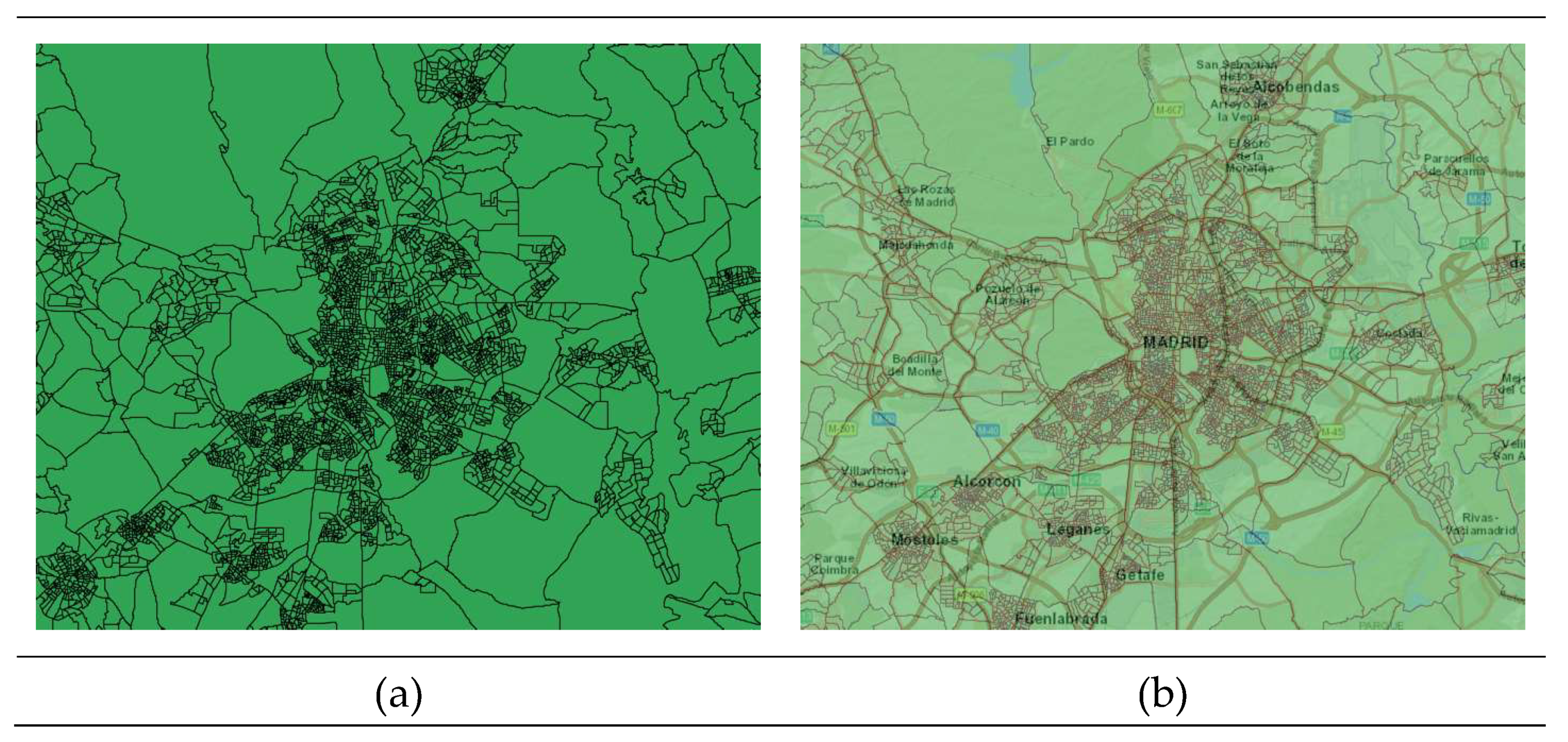
4.1.5. Cartography of the Spanish Institute for Statistics (INE)

The INE does not have a specific section for the management of spatial data. These are available in different pages and, sometimes, in a confusing way. First, it is increasingly common for INE to include viewers to look at certain variables, as is clearly the case in the “Territorial Statistics” section (although there are also viewers in other sections such as “Experimental Statistics”). In addition, practically all data tables with spatial information (generally offered in Ms. Excel format) usually have the corresponding official code of autonomous communities, provinces, municipalities, districts or census sections or tracts, as appropriate. This makes it possible to cross-reference the content of these tables with the digital maps, provided that these maps also contain the official codes (which is almost always the case). Finally, the INE also delivers digital maps in accessible formats, such as Shapefile.

a)

Population in 1 km2 cells and associated digitalized cartography.

This is a file in Shapefile format that contains the 115,410 grids of 1 km2 of the Spanish entities where there is a resident population (INE 2025a).

b)

Cartography of the Censal Sections.

It is a group of files which contains the digitalization of the georeferenced outlines of the censal sections, according to UTM projection, zones 28, 29, 30 and 31 North (INE 2025b). The files are available in ESRI’s formats like Shapefile. They contain nationwide data for a census tract scale and are accessible annually since 2001.

c)

Electoral Census Street Map.

It covers all information that fully identifies the branches that belong to each census section (INE 2025b). As additional information it includes the postal district of each branch in question. This is a set of four files (in ASCII format): street files, pseudo street files, street portion file and population unit file. Information on the content and processing of the text file can be found on the website, under the name “registry design”. The files, which contain nationwide data for a street scale, are available annually since 2004 (dated January) and, since 2011, semiannually (dated January and July). However, the name “map” here is confusing since this information is not offered in any digital map format, so it cannot be visualized. As far as we know, there is no digital street map for the whole Spain, but they can be found in statistical portals of some cities and regions, such as Madrid.

4.2. GEOGRAPHIC INFORMATION SYSTEMS (GIS)

GIS means Geographic Information System. It is software that brings together maps and data for analysis, to better understand the world around us. GIS mapping allows people to create, manage, and analyze information about a location (Ordnance Survey 2025). Hence, a GIS is used to link data to locations. Approximately 80% of all information held in databases anywhere in the world contains some kind of geographic element. For example, records relating to an address, a building, property, or a road track.

There are many trends and relationships hidden in this geographic data, but it is only by using a GIS that these can be revealed. Many companies use GIS technology as a central part of their activities, with an extraordinary range of applications in use. The GIS stores information about geometry, the shape and location of the objects, and attributes, the descriptive information known about the objects, normally displayed on a map through symbology and annotation.

For this information to be read by computers, it is stored in digital form as raster and vector data. Next, some of the most important and widely used GIS platforms are presented.

4.2.1. ArcGIS Pro

ArcGIS Pro is the ESRI’s proprietary desktop GIS application. It only runs on Ms. Windows. There are several prices depending on the user's needs, the advanced analysis extensions to be installed, and the country from which the software is requested. In addition, ArcGIS Pro licenses are also available for schools and universities (e.g., UAM provides student and faculty accounts upon request to the User Service Center (cau@uam.es). See ESRI (2025d).

It is used to transform data into maps combining multiple data sources to make maps that are smart and beautiful. It can integrate tabular data, drawings, cloud data warehouses, recognizing various formats. Interactive tools help you to create objects by clicking on the scene or using input layers. It offers unparalleled tools to work with spatial data effectively, generating 2D, 3D, and 4D visualizations (spatiotemporal trends in a long, width and height representation). Hence, it allows conducting advanced mapping analytics to identify patterns, make predictions, and answer questions. It is also possible to automate work with “ModelBuilder” (ArcGIS’s visual programming language) or the ArcGIS Pro libraries for Python.

The data sharing of projects and information within the ArcGIS system fosters valuable GIS solutions and insights within an organization, online, and through mobile apps (ESRI UK 2025).

4.2.2. QGIS (Quantum GIS)

QGIS is a GIS renowned for its powerful robust capabilities in spatial data analysis, mapping, and visualization (BEEILAB 2005). It is freely available, that is, accessible to everyone from its download web page (QGIS 2025). QGIS is a versatile inclusive software which runs on Linux, Unix, Mac OSX, Windows and Android and supports numerous vector, raster, and database formats.

It is an open-source software that operates under a GNU General Public License (Tobias 2024). That means the code is available for everybody to read or modify if needed, though it is not necessary. Hence, it is continuously developed by a global community whose make fixes if something is wrong or add new features. It is also one of the official projects of the Open-Source Geospatial Foundation (OSGeo), which is a not-for-profit organization whose mission is to foster global adoption of open geospatial software. It provides infrastructure and organization, as well as conferences and means of communication with the broader public and education.

QGIS is a user-friendly desktop GIS, that is, a program that opens up on a computer as a window with buttons to click, forms to fill out to do tasks, etc. It is a visual interactive experience, as opposed to commandline programming in a terminal. This kind of interface is called a “Graphical User Interface” (GUI). It allows selecting a vast collection of plugins, extending functionality to tailor QGIS to specific needs and applications.

4.2.3. MapInfo Pro

MapInfo Pro is a proprietary GIS program that is widely used in universities, municipalities, institutions and private institutions across the world, especially in infrastructure companies (Başarsoft 2024). It is the world’s most user-friendly and easy-to-use GIS program, a very easy program to learn and work with. Without going into complex structures, it enables easy integration of especially beginners into GIS with interface where all functions can be found easily. Like ArcGIS Pro, It only runs on Ms. Windows. With improved interface, enables the creation of perfect maps faster and easily so as business analysts, GIS professionals and even non-GIS users can make the right strategic decisions.

MapInfo Pro Viewer allows users to open and view any MapInfo Pro project file. One can perform basic map operations such as panning, zooming, or reordering layers by opening additional tables in read-only mode. Productivity can be increased by building and running customized applications with Python. It also allows creating and saving custom queries using MapBasic scripts.

The MapInfo Pro Advanced module allows measuring and visualizing large raster data. It offers many raster analysis and mathematical modeling tools, along with the MRR (Multi Resolution Raster) proprietary raster compression technology to handle extremely large file sizes. Users can perform data integration modeling and visualization between vector and raster fields in the same software.

Being a proprietary program, MapInfo Pro has a cost, but it is not possible to know the possible subscriptions, as they invite those interested to contact Precisely directly, through the web. But there is a full free 30-day trial version available (Precisely 2025).

4.2.3. Google Earth Pro

The enhanced version of the viewer Google Earth, Google Earth Pro, is a powerful free geographic information system software with which it is possible to explore the Earth as a virtual globe created thanks to high-quality cartographic data and satellite images. It is often preferred over Esri’s ArcGIS Pro or QGIS for its advanced features and accessibility (Softonic 2025). Google Earth Pro has a myriad of tools.

Interface is intuitive, it has a clear and simple interface, from which it is possible to easily scroll, zoom, and explore the planet. Image and map visualization allows to navigate, explore, and observe in detail any corner of the planet having access to a myriad of satellite images, aerial photographs, 2D and 3D maps, and historical images showing changes and evolution of each area of the planet.

It also has advanced GIS options, allowing to import geographic data from in KMZ or KML formats, add layers of information, and perform analysis of with some measurement tools of the area, radius, and length of any zone or building on the planet (Fig. 4), creation of tours and custom videos (e.g. before preparing a trip), as well as generate interesting videos to download from the application.

Finally, Google Earth Pro is a multi-platform GIS compatible with computers running Windows, Linux, or MacOS operating systems.

Figure 4. Length between Toledo and Madrid (Spain), Google Earth Pro.

Figure 4. Length between Toledo and Madrid (Spain), Google Earth Pro.

To download Google Earth Pro, simply access the Google Earth portal, accept the privacy policy of the service, and download the application at no cost (Google Earth 2025). The latest update to Google Earth Pro provides a toolbox of new features and improvements.

4.3. INTRODUCTION TO GEODA SOFTWARE

GeoDa was developed by Dr. Luc Anselin and his team. It is a free and open-source software tool that serves as an introduction to spatial data science (Anselin 2025). Although over the years –since its creation in 2003– it has incorporated many GIS functions, it is not a GIS per se, but a spatial data analysis software.

GeoDa is designed to be user friendly and intuitive, working through a graphical user interface (GUI). A distinctive characteristic of GeoDa is the implementation of dynamically linked graphs, in the sense that one or more selected observations in a “view” of the data (a graph or map) are immediately also selected in all the other views, allowing interactive linking and brushing of the data. This GUI is provided to methods of exploratory spatial data analysis (ESDA) and basic spatial regression models. It is an inclusive multisystem software which runs on Linux, Mac OSX, and Windows, and supports numerous vector, raster, and database formats.

The latest version contains several new spatial analysis methods and the following GIS functionalities (Anselin 2023):

a) Numerous vector and database formats allowing importing, converting and exporting various formats. Specifically, it can import shapefiles, geodatabases, GeoJSON, MapInfo, GML, and KML, among others. It can also make coordinate conversion in table format (.csv, .dbf, .xls, .ods) to a spatial data format, as well as data conversion between different file formats (such as .csv to .dbf or shapefile to GeoJSON). Finally, GeoDa can export a subset of a table or a map as a new file.

b) Multilayer support, that is, it can load additional layers only for visualization purposes (for the time being), but the analysis functions are done on the layer firstly loaded. Besides, GeoDa can add a basemap to any map view, if the map is projected (*.prj file), for better orientation and for ground-truthing results (Fig. 4).

c) Finally, GeoDa makes an efficient treatment of projections. It computes minimum spanning trees and makes spatial aggregation and spatial join through multi-layer support.

Figure 4. Sensus sections map of Madrid without (a) and with (b) a basemap, GeoDa.

Figure 4. Sensus sections map of Madrid without (a) and with (b) a basemap, GeoDa.

5. CONCLUSIONS

This paper has delineated the multifaceted aspects and applications of geospatial analysis, highlighting its indispensable role in business analytics, urban planning, network optimization, competitive intelligence, and more. Geospatial data offers a unique vantage point by integrating the dimension of space, allowing for a nuanced understanding of various phenomena that traditional data analysis might overlook. The integration of location data into predictive models not only enriches the analysis but also enhances the accuracy of predictions, ensuring more informed decision-making processes.

Spatial data differs fundamentally from time series data in its dimensions, scales, and references. While time is linear and one-dimensional, space is bidirectional and exists in 360 degrees. Geographic space can be divided into various administrative scales, exemplified by the EU's NUTS system and Spain's territorial divisions. Spatial data requires specific referencing systems using latitude-longitude coordinates and appropriate projections. Two main types exist: raster data (grid cells) and vector data (points, lines, and polygons).

Digital maps come in both proprietary and open-source formats. Proprietary formats include ESRI's Shapefile and Geodatabase, and MapInfo's TAB files. Open-source formats include GeoArrow, GML, GeoJSON, GeoPackage, GeoParquet, KML, and SpatiaLite. These formats differ in data organization (row-oriented, column-oriented, or hierarchical), size limitations, and support for vector and raster data. Map viewers allow users to interact with geographic information online through functions like zooming, layer control, searching, and data visualization.

The technological platforms discussed, such as ArcGIS, QGIS, and GeoDa, facilitate the manipulation and visualization of geospatial data, each offering tools tailored to different professional needs and expertise levels. These platforms are instrumental in democratizing access to geospatial analytics, allowing users from varied industries to adopt and integrate geospatial data into their workflows effectively.

In conclusion, the power of geospatial analysis lies in its ability to add a spatial dimension to traditional analyses, offering a more comprehensive view of data and its real-world applications. This integration enriches our understanding and decision-making capabilities, proving essential in an increasingly data-driven world.

References

- Anselin. An Introduction to Spatial Data Science with GeoDa Volume 1: Exploring Spatial Data. 2023. Available online: https://tinyurl.com/zrc8afa3.
- Anselin. Introducing GeoDa 1.22. GeoDa An Introduction to Spatial Data Science. 2025. Available online: https://geodacenter.github.io (accessed on 1 January 2025).
- Başarsoft. MapInfo Pro. The World's Most Flexible, Extensible GIS Software. 2024. Available online: https://tinyurl.com/nhcypcc4 (accessed on 1 January 2025).
- BEEILAB. What is QGIS? Exploring the Power of Quantum GIS. 2025. Available online: https://tinyurl.com/mryrwamv (accessed on 1 January 2025). Medium.
- Chasco C, Fernández-Avilés G. Análisis de datos espacio-temporales para la economía y el geomarketing. 2009. Ed. Netbiblo. Available online: https://tinyurl.com/2uyamf2n.
- ESRI. Esri Grid format. 2024. Available online: https://tinyurl.com/4buzr9nr (accessed on 1 December 2024).
- ESRI. ArcGIS Living Atlas of the World. 2025. Available online: https://livingatlas.arcgis.com/en/browse/#d=2 (accessed on 1 January 2025).
- ESRI. Map Viewer. 2025. Available online: https://tinyurl.com/5n8p2z5k (accessed on 1 January 2025).
- ESRI. ArcGIS Hub. 2025. Available online: https://hub.arcgis.com/search (accessed on 1 January 2025).
- ESRI. Pricing for ArcGIS Pro. 2025. Available online: https://tinyurl.com/3f584bzh (accessed on 1 January 2025).
- ESRI Developer. Geocoding. 2024. Available online: https://tinyurl.com/5n6dxuck (accessed on 1 December 2024).
- ESRI UK. ArcGIS Pro. The world's leading GIS software. 2025. Available online: https://tinyurl.com/236uh4sm (accessed on 1 January 2025).
- Eurostat. GISCO Grids. 2024. Available online: https://tinyurl.com/54dvyupv (accessed on 1 December 2024).
- Eurostat (2024b) Local administrative units (LAU). Accessed in December 2024. Available online: https://tinyurl.com/4y9srkvf.
- Eurostat (2024c) NUTS - Nomenclature of territorial units for statistics. Overview. Accessed in December 2024. Available online: https://tinyurl.com/7ktnn82v.
- Eurostat (2025) GISCO Geodata. Accessed in January 2025. Available online: https://tinyurl.com/4cyj4kx6.
- GADM (2022) GADM data. Available online: https://gadm.org/data.html.
- Geoapify (2024) Online geocoding tool. Accessed in December 2024. Available online: https://tinyurl.com/ypwtsm4u.
- GeoArrow (2024) GeoArrow. Accessed in December 2024. Available online: https://geoarrow.org.
- GeoMap (2025) GeoMap.com. Accessed in January 2025. Available online: https://www.geamap.com/en.
- GISGeography (2024) Vector vs Raster in GIS: What’s the Difference? Accessed in December 2024. Available online: https://tinyurl.com/38a485yb.
- Google Earth (2025) Download Google Earth Pro. Accessed in January 2025. Available online: https://tinyurl.com/4rfr9mny.
- Google Maps Platform (2024) Geolocation API overview. Accessed in December 2024. Available online: https://tinyurl.com/4bp6je9a.
- INE (2025a) Population in 1 km2 cells and associated digitalized cartography. In Population and Housing Census 2021. Advanced query system. Accessed in January 2025. Available online: https://tinyurl.com/52j85hmk.
- INE (2025b) Cartography of the Censal Sections and Electoral Census Street Map. Accessed in January 2025. Available online: https://tinyurl.com/2dhmtu8u.
- Johns Hopkins (2025) COVID-19 Dashboard. Center for Systems Science and Engineering (CSSE). Accessed in January 2025. Available online: https://coronavirus.jhu.edu/map.html.
- Ministerio para la Transformación Digital y de la Función Pública (2024) GeoParquet 1.0.0: new format for more efficient access to spatial data. Accessed in December 2024. Available online: https://tinyurl.com/y33sjs4c.
- OpenStreetMap Foundation (2025) OpenStreetMap. Accessed in January 2025. Available online: https://tinyurl.com/3cv3c9jv.
- Open Geospatial Consortium (2024) GeoPackage. An Open Format for Geospatial Information. Accessed in December 2024. Available online: https://www.geopackage.org.
- Ordnance Survey (2025) What is GIS? Accessed in January 2025. Available online: https://tinyurl.com/4767mzpr.
- Precisely (2024a) Geo Addressing. Accessed in December 2024. Available online: https://tinyurl.com/jfvh9tte.
- Precisely (2024b) MapInfo Pro. Accessed in December 2024. Available online: https://tinyurl.com/4ykpdsj6.
- Precisely (2024c) Multi Resolution Raster (MRR) - Revolutionizing Raster Performance and usage. Accessed in December 2024. Available online: https://tinyurl.com/5fz9e62t.
- Precisely (2025) MapInfo Pro 30-Day Free Trial. Accessibility in January 2025. Available online: https://tinyurl.com/5ybce87v.
- QGIS (2025) QGIS download web page. Accessed in January 2025. Available online: https://www.qgis.org.
- SAFEGRAPH (2024a), Geospatial Data Analytics: What It Is, Benefits, and Top Use Cases. Web page accessed in December 2024. Available online: https://tinyurl.com/49667hs7.
- SAFEGRAPH (2024b), Top 10 Uses of Geospatial Data + Where to Get It. Web page accessed in December 2024. Available online: https://tinyurl.com/yc5rap78.
- Softonic (2025) Google Earth for Mac. Accessed in January 2025. Available online: https://tinyurl.com/32kphz2b.
- Tobias M (2024) What is QGIS? In: Intro to Desktop GIS with QGIS. 2024-05-14. Available online: https://tinyurl.com/yrkh3ux6.
- United States of the Interior (2025) USGS, U.S. Geological Survey. Accessed in January 2025. Available online: https://apps.nationalmap.gov/downloader/#/.
- Warmerdam F, Rouault E & others (2025) RasterLite2 – Rasters in SQLite DB. Accessed in January 2025. Available online: https://tinyurl.com/2tzyy6cy.
- Wikipedia (2024a) Nomenclature of Territorial Units for Statistics. Accessed in December 2024. Available online: https://tinyurl.com/5n9xmdmv.
- Wikipedia (2024b) Geodatabase (ESRI). Accessed in December 2024. Available online: https://tinyurl.com/bdzbdhwe.
- ikipedia (2024c) Geography Markup Language. Available online: https://tinyurl.com/52xbcb88.
- Wikipedia (2024d) Keyhole Markup Language. Accessed in December 2024. Available online: https://tinyurl.com/yc3vtwd5.
- Wikipedia (2024e) SpatiaLite. Accessed in December 2024. Available online: https://tinyurl.com/3d8h3yhz.