1. Introduction
The study of terrain visibility is an interdisciplinary field that combines knowledge from various domains such as Geographic Information System (GIS), computer graphics, remote sensing technology and spatial analysis. It aims to predict and analyze the range of terrain visible from a specific location through mathematical models and computational methods. Visuality analysis refers to the processing of the visual perception and cognition of target objects by the human eye into a type of geographic information, where the concept of visibility involves whether it is visually reachable. Through the calculation of the viewshed of terrain [
1,
2], It has numerous applications like security, surveillance, forest fire lookout station setup and navigation. Many scholars have conducted extensive research based on visibility, including military defence, ecological studies, urban planning, and disaster management. In military defence, it can be used to assess the location of observation posts and identify blind spots in surveillance [
3,
4]. In ecological research, it can be used to analyze the visibility of animal habitats and evaluate the impact of human activities on them [
5,
6]. In urban planning, it can help select the optimal location for buildings to ensure landscape harmony and open views [
7]. In disaster management, especially in forest fire prevention, maximizing the visibility range of observation posts is crucial [
8]. The minimum number of observation points can be established through visibility analysis techniques to maximize the monitoring range or assess the visual range of rescue points to optimize emergency response strategies.
Geospatial semantic relationships are one of the core concepts in the field of geographic information systems and spatial science. They refer to the interrelationships in space and the semantic information these relationships convey. These relationships not only describe the topological relationships between geographical entities but also encompass their semantic connections, enabling geographic information systems to understand and analyze geographic data more deeply. Scholars have conducted extensive research on geospatial semantics. Margarita and others summarized the research on modeling and extracting geospatial semantic information, emphasizing the importance of ontology in knowledge representation and information extraction [
9]. Spatial semantic relationships can be applied to the identification of urban functional zones, using spatial semantics and interactions to recognize urban functional areas, enhancing the understanding of urban structures [
10]. In natural language processing, they can be used in the study of spatial relationship word analysis models in Chinese texts, aiding in the semantic integration of GIS and natural language [
11]. In geographic information systems, they can be utilized for research and application of geospatial semantic ontology knowledge bases, providing more precise geographic information data for GIS [
12]. Common geospatial semantic relationships include topological relationships, metric relationships, and semantic functional relationships. Spatial topological relationships describe the positional relationships between spatial elements without relying on their exact latitude and longitude coordinates [
13,
14]. The metric relationship involves distance and orientation in the spatial element, i.e., the distance between spatial entities and the angle of direction between them. Functional relationships usually refer to the functional linkages and interactions between different spatial units in fields such as architecture, urban planning, and geographic information systems.
Existing methods of viewshed representation include the visible graph and visible neighborhood configuration. The visible graph [
15] is a tool for time series analysis that maps time series onto complex networks and uses graph theory to study problems. From the initial point, it observes the surrounding visible points and calculates the next visible point based on visible points until the target point is reached. It is suitable for solving shortest paths, line of sight corridors. The visible neighborhood configuration [
16] is a new method of exploring the complex theory of landscape visual phenomena by processing the total viewshed, this method involves the configuration of visual attributes of the location itself and the surrounding locations. It introduces a neighborhood around the viewpoint with a given shape, size and visibility structure. It calculates the degree of conformity between the actual visibility of the area around the viewpoint and this neighborhood, enabling people to describe the visibility characteristics of the surrounding area. Common visibility structures include unified viewshed, distance band, gradient, direction, etc. The unified viewshed means that within a fixed range around the viewpoint position, the visibility of each position is equal. The distance band implies that the visibility value changes with the specified distance. But within a fixed distance range, its visibility value is constant. The gradient means that the visibility value gradually changes with distance. As the distance between grid points and the viewpoint position increases, visibility also gradually increases or decreases. Directional attributes refer to the fact that the viewshed presents a directionality and different directions have different visibility at the viewpoint. That is, standing at the viewpoint position, observers can only see the landscape area in one direction of the viewpoint position, while the visibility in another direction is different.
The terrain viewshed is regarded as an object collection from a viewing point or multiple visible points, and this representation lacks a qualitative description of the spatial distribution of visible objects, let alone the semantic information of the view. Based on our analysis of the spatial relationship of the viewshed, the viewshed presents local clustering on the terrain, forming sub-viewsheds after partitioning. Therefore, this paper attempts to propose a new semantic representation model for terrain viewsheds through these sub-regions. The article aims to establish a sub-viewshed spatial semantic representation model to represent the relationships between visible sub-viewsheds. By using the DBSCAN algorithm to cluster view data, defining a series of attributes characterizing sub-viewshed features for spatial analysis, and establishing a spatial semantic structure diagram of sub-viewsheds, it provides a feasible approach for establishing a quantitative and qualitative description model of the view. This paper proposes a general method for expressing the spatial semantics of the view. A formal expression of the viewshed is established by using a series of attribute parameters representing the characteristics of the viewshed and high-precision DEM (Digital Elevation Model) data as background. Finally, the divided viewsheds are displayed in the form of three-dimensional views on the terrain map, allowing non-professionals to clearly understand the information related to the viewshed in an easy-to-understand way.
2. Research Area, Data Sources and Processing
Purple Mountain, alternatively referred to as Zhongshan in Nanjing, was historically recognized as Jinling Mountain. Positioned within the Xuanwu District of Nanjing, its coordinates span from 118.8° to 118.951° east longitude and 32.033° to 32.104° north latitude. The mountain’s expanse extends from east to west by approximately 7 kilometers and from south to north by up to 3 kilometers, forming a triangular shape with its peak pointing north on the plane. The terrain is characterized by low mountains and hills, complemented by broad foothills that extend on both the southern and northern slopes, resulting in a sloping surface. The elevation increases near the mountain body and decreases further away. A few low mountains and hills are scattered in the surrounding areas, contributing to the relatively flat overall terrain.
Purple Mountain belongs to the middle branch of the Ningzhen Mountain Range’s western section, generally referred to as the low mountain and hilly area between Nanjing and Zhenjiang. It is located on the south bank of the Yangtze River, starting from Qinglong Mountain in Jiangning District of Nanjing and Mufu Mountain in Nanjing, passing through Jurong, Dantu, Zhenjiang, and Danyang, and ending at Huangshan in Menghe Town, Wujin District of Changzhou. It stretches for 100 kilometers, with an average altitude of 200-400 meters. The highest peak is the North Peak of Zhongshan, with an altitude of 448 meters. The western section is more comprehensive and mainly consists of low mountains, while the eastern section is narrower and primarily composed of hills.
This study obtained 12.5m precision topographic data of Nanjing from the Tuxingis platform (
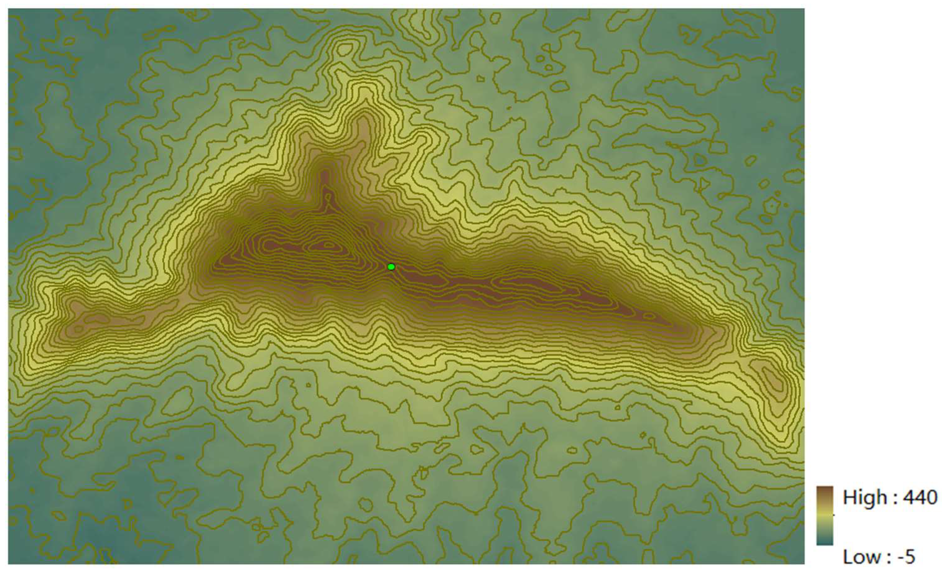
http://www.tuxingis.com) and used ArcGIS software to process, analyze and visualize the data. Firstly, the experimental data was cropped to obtain the terrain of Purple Mountain, with a cropping range between 118.819°E to 118.875°E longitude and 32.049°N to 32.089°N latitude and an elevation range from -5 meters to 440 meters, The contour interval is 12.5 meters.
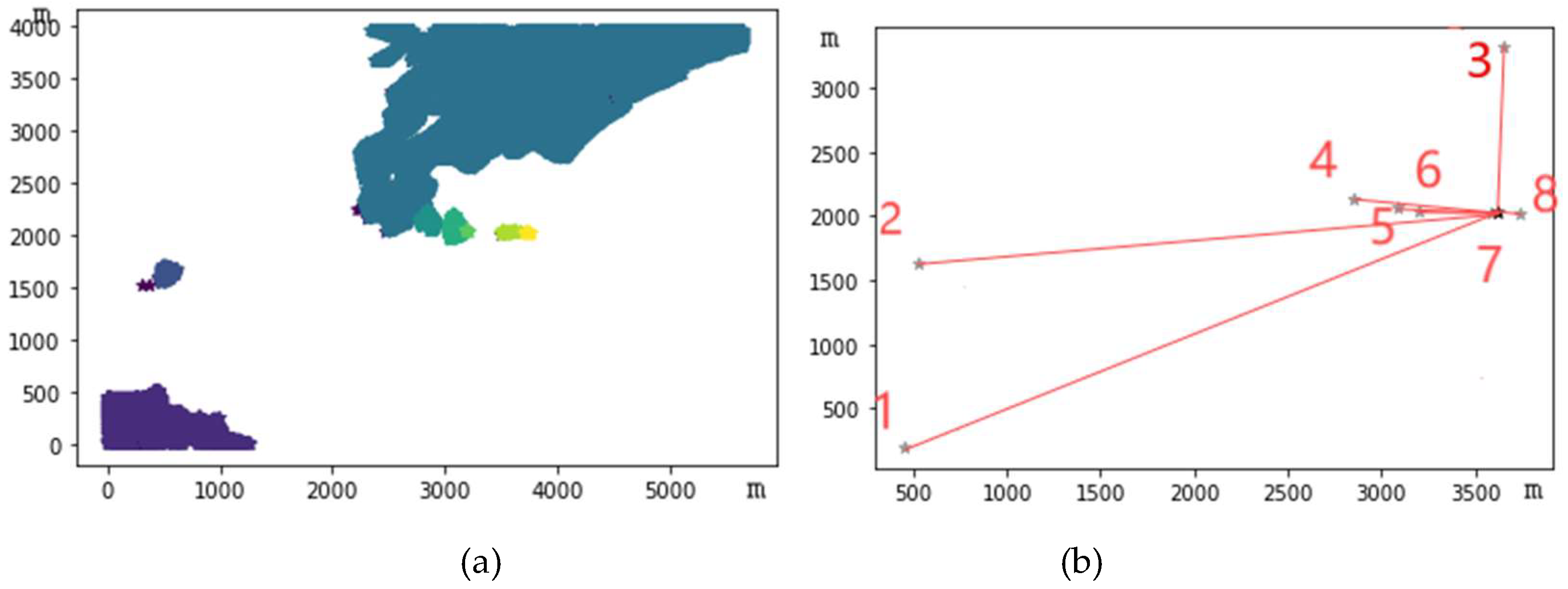
To enhance research efficacy in the Purple Mountain area, it is necessary to carry out corresponding clipping. An observation point is set at coordinates (118.85°, 32.078°), with an elevation of 334 meters, located on the mountainside. The terrain data and the position of the observation point are depicted in
Figure 1, where the origin signifies the observation point. In
Figure 1, the darkest section in the center of the Purple Mountain denotes high-altitude areas. The terrain extends east to west, with higher altitudes forming a ridge line. The altitude gradually decreases to varying degrees towards the north and south, resulting in watersheds and catchment areas.
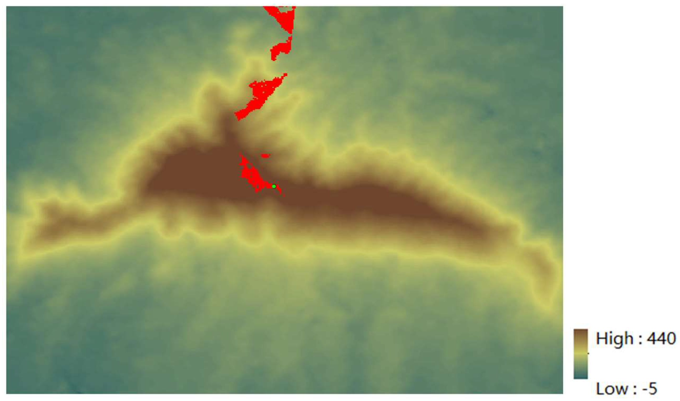
ArcGIS is a powerful GIS processing tool, serving as a leading platform for the construction and application of geographic information system. It allows users to collect, organize, manage, analyze, communicate and publish geographical information. In this experiment, the viewshed analysis function of ArcGIS is utilized to conduct a viewshed analysis on the observation point location. After filtering out the visible area, we obtained the results shown in
Figure 2. The viewshed is primarily concentrated in the north-sight direction from the observation point. In this direction, the field of view at the observation point location is relatively straightforward with less obstruction. However, other places are unreachable due to significant elevation differences between them and the observation point, making them invisible to the observer. After data processing, we exported Purple Mountain DEM, observation points and the viewshed data into raster data for further experiments.
3. Terrain Viewshed Spatial Semantic Expression Model and Feature Extraction
The viewshed is a set of visible points relative to the observation point for a single viewpoint. From the perspective of the DEM data model, the viewshed is a group of visible grid units on the terrain, which can be represented by three-dimensional coordinates (x, y, z) x and y represent the ground coordinates on the grid unit and z represents the elevation value of the grid unit. Zhao analyzed the spatial vision characteristics of a memorial hall through the method of spatial quantitative analysis, but it was only based on the analysis of the two-dimensional plane, and did not take the viewshed characteristics of the complex three-dimensional space into account [
17]. The viewshed is scattered on the terrain surface and traditional set representation methods cannot qualitatively and quantitatively express its implicit topological features. In the field of real-time visibility computation, scholars have proposed voxel-based visibility analysis and rapid visibility computation methods. These can handle large-scale terrain model visibility calculations under real-time conditions. However, this method has not yet been effectively applied in the evaluation of the geometric morphology of the visible terrain [
18]. Observing the viewshed of viewpoints in the terrain shows that the visible points or units in the viewshed have local accumulation properties. These visible units become multiple continuous regions or single outliers or micro-regions composed of several points. Calculation errors in the viewshed may cause these outliers or micro-regions or a few scattered discrete points that can be ignored. Therefore, based on three-dimensional space, the viewshed of the viewpoint is abstracted into a series of separate sub-viewsheds with different sizes and shapes. Then, the characteristics and mutual topological relationships of these sub-viewsheds are studied to establish quantitative expression and qualitative description models and methods for the viewshed of the viewpoint.
Utilizing the method of regional division, visual units are segmented into multiple aggregated sub-view fields. Visual points within the same sub-viewshed exhibit aggregation, whereas those in different sub-view fields display dispersion. A model that describes the spatial semantic distribution characteristics of the viewshed is established based on the feature distribution of the viewshed, as depicted in Equation (1).
TV(O) represents the viewshed of observation point O, and Vi ( i =1, 2, …, n) represents each sub-viewshed following division, where n signifies the total sub-viewshed. The visible points across all these sub-viewsheds collectively constitute the comprehensive viewshed set for the observation point. The spatial semantic characteristics articulated by each sub-viewshed contribute to forming the spatial feature distribution within the observation point’s viewshed.
3.1. Spatial Semantic Composition
The visual range observed from a certain observation point is divided into multiple smaller viewsheds, and each of these smaller viewsheds after division is called a sub-viewshed. Tandy first proposed the concept of lsovist viewshed analysis, defining the lsovist as the set of all points visible from a certain point in space. Later, Benedikt introduced the theoretical methods and framework for lsovist viewshed analysis, quantifying parameters such as the area, perimeter, richness, and occlusion ratio of the viewshed by calculating different information about the space at different observation points [
19,
20]. In three-dimensional space, mere metrics like area and perimeter are insufficient. To measure the characteristics of the observation and its sub-viewshed, as well as the spatial semantics of the sub-viewshed themselves, more indicators are needed to quantify their features, such as the size, shape, center point, and distribution sparsity of the viewsheds. By defining a series of spatial attributes of the sub-viewshed, such as the topological relationship and the metric relationship between the sub-viewshed, the spatial semantic relationship of the viewshed is finally formed. The spatial semantic characteristics of the sub-viewshed Vi (i =1, 2, …, n) can be quantitatively described using the following method:
(1) Shape: The spatial geometry formed by the visible terrain units of a sub-viewshed, which can be represented by the boundary contours distributed by the visible point grid. Then connecting the points adjacent to the outer boundary of each sub-view can obtain the shape of the sub-view. We can judge the sparsity of viewpoint distribution by the shape of sub-viewshed.
(2) Area: The area of a sub-view can be represented by the projected area, denoted as Si (i =1, 2, …, n), The area of the sub-viewshed can be obtained by multiplying the number of visible grid points within the sub-viewshed by the precision of the terrain.
(3) Number of Visible Units: The number of visible units is denoted as the number of visible points in that sub-viewshed.
(4) Density: The proportion of visible units in a given sub-view area to all visible units in the entire view area. Calculating the density of a sub-viewshed can be used to measure how sparsity the sub-viewshed is distributed across all viewsheds.
(5) Center: Center refers to the central coordinate of the sub-viewshed, which is denoted by the mean value of all visible units within the sub-viewshed.
(6) Azimuth: The position of the center of a sub-viewshed relative to the viewpoint or observation point, typically represented by the distance and angle between the center of the sub-viewshed and the viewpoint. Using the southwest edge angle of the terrain as the coordinate origin, due east is 0° azimuth. The azimuth relationship is expressed in polar coordinates.
(7) Sparsity Level: The sparsity level of visible points within the field of view can be characterized by the average distance and the center distance within sub-viewshed.
Average distance: The ratio of the sum of the Euclidean distances between any two visible grid points in the sub-viewshed V
i to
(where
represents the square of the number of visible points in a sub-viewshed.), as shown in Equation (2):
The mean distance within a sub-viewshed serves as an indicator of the sparsity of visible points.
The sum of central distance: The central point of the sub-viewshed
is denoted by
. The ratio of the sum of distances from each visible point to the center point in a sub-viewshed to
, as depicted in Equation (3).
The average distance and the sum of central distance can better describe the distribution of visible points in the sub-viewshed.
(8) Topological Relationship Between Sub-viewshed and Observer
A topological relationship graph is established between the observation and the sub-viewshed, with the observation point at the center. Each sub-viewshed has a specific relationship to the viewpoint, such as being in a direction or at a certain distance from it. In other words, from the viewpoint position, one can observe a specific sub-viewshed from a direction relative to the observer. This sub-viewshed also possesses distinct attribute characteristics.
3.2. Space Semantic Feature Extraction Based on Cluster Analysis
The Density-Based Spatial Clustering of Applications with Noise (DBSCAN) algorithm is designed for spatial data clustering and is particularly effective in analyzing terrain data with spatial characteristics [
21]. The process involves identifying clusters by examining the vicinity of each data point within the dataset. During computation, all data points must be traversed. Each point is initially designated as unvisited. Upon visiting a point, it is marked as visited and the count of points within its vicinity is determined using a distance formula. If this count exceeds the minimum sample size, the point is classified as a core point. If not, the algorithm reverts to the next unvisited point. If a point is identified as a core point, its neighboring points are categorized to form a class centered on that point. This class is then assigned a new label and the process continues with the points within its vicinity until all points have been visited, at which point the algorithm concludes [
22]. Due to the irregular shape and significant differences in terrain data, we cannot know the number of subregions at the beginning. The DBSCAN algorithm does not require predetermining the number of clusters and can cluster data of any shape. Furthermore, DBSCAN can ignore outliers, which helps us maintain the main subregions of the visual field. Therefore, choosing DBSCAN is a more appropriate clustering algorithm.
The DBSCAN algorithm is characterized by two parameters: Eps and MinPts. Eps denotes the neighborhood radius, signifying that the points within this radius can merge into a cluster. This parameter serves as a threshold for determining whether data objects can be grouped, reflecting the smoothness between two adjacent grid points. A slight elevation difference between two neighboring grid points suggests that the terrain in the area is relatively flat, while a significant difference indicates a steep slope. MinPts represents the minimum number of sample points required to form a cluster. A cluster can be formed if the number of points within the neighborhood radius surpasses this minimum; otherwise, these points are classified as noise data. Due to the complexity of the terrain, the slopes of different terrains cannot be accurately measured. Generally, the slopes of hilly terrains are relatively gentle, but the slopes in steep hilly areas generally do not exceed 50°. Consequently, the center distance between two adjacent grids can be calculated using equation (4), where D represents the maximum value of the neighborhood parameter, and R represents the precision of the terrain grid.
After determining the range of the neighborhood radius, it is necessary to decide on the MinPts parameter. Since noise data is generated due to a small part of computational errors, parameters with as little noise data as possible should be selected. The minimum sample points should be reduced as much as possible to minimize noise data. At the same time, the chosen minimum sample points should not cause a “cliff-like” change in the number of clusters. The selection of cluster numbers that vary with less changes in the neighborhood can better reveal the relationship between the number of clusters and the parameters chosen for MinPts and Eps. When MinPts=1, even if the distance between any point and its adjacent points in the data exceeds Eps, it can form a cluster. Currently, the computation is meaningless. Consequently, calculations within a fixed neighborhood range commence with MinPts set at 2. The choice of Eps must balance noise variations and cluster count changes. Once Eps is established, noise levels should remain relatively low and not experience substantial fluctuations subsequently. This paper conducts visibility analysis from a single viewpoint. If clustering analysis needs to be performed on other multiple visible points in the terrain, the existing DBSCAN parameters are also applicable.
4. Experimental Analysis
The precision of the terrain data in this experiment is 12.5 meters. Using the calculation formula of the neighborhood range, the Eps range for the experiment should fall within [
13,
20].
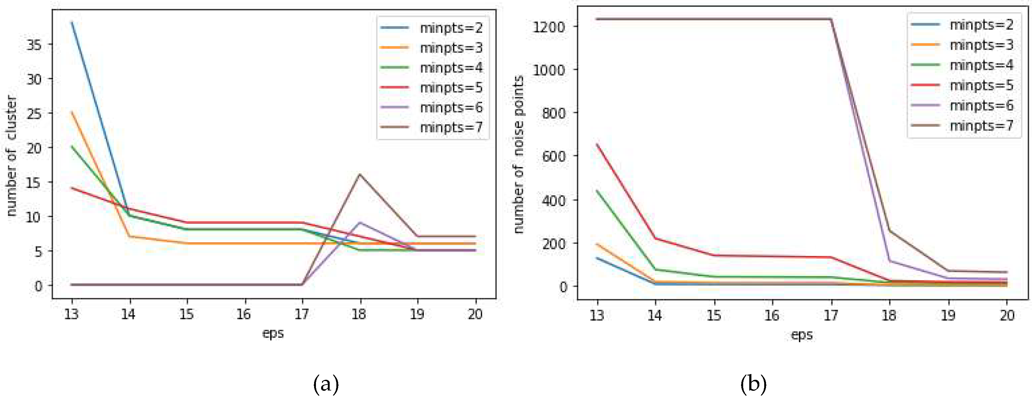
Figure 3 illustrates the fluctuation in the number of clusters and noise data as the neighborhood radius varies when MinPts lies between 2 and 7.
Figure 3 illustrates the outcomes of the cluster analysis.
Figure 3(a) and
Figure 3(b) depict the number of clusters and noise points derived from clustering under varying parameters such as neighborhood radius Eps and minimum sample points MinPts. As indicated in
Figure 3, there is a fluctuation in the number of clusters under different minimum sample points. When MinPts is 6 and 7, and Eps is 17 or 18, the number of clusters and noise points shows significant changes but remains unchanged as parameters increase further. Consequently, this parameter is not beneficial for parameter selection and should be excluded. Similarly, when MinPts equals 2 or 3, the number of clusters also experiences a sudden change before stabilizing. In that case, there are fewer noise points, but the number of clusters suddenly decreases with changes in the neighborhood radius. This is attributed to isolated noise points whose quantity exceeds two, and these two or more points are proximate. They are classified into a cluster under a lower neighborhood radius Eps. As the neighborhood radius increases, the genuine clusters merge the classes composed of noise data. This situation can misguide the choice of Eps results; hence, it needs to be excluded. When MinPts equals 4 or 5, neither of these situations occurs that will cause a significant change in the number of clusters. However, when MinPts equals 5, the volume of noise data surpasses that when MinPts equals 4, as shown in
Figure 3(b). Given that this study focuses on the viewshed and aims to incorporate more visible points in subsequent analysis, it is currently necessary to have relatively fewer noise data and include more visible points in the viewshed analysis. Therefore, choosing MinPts as 4 is more rational, and with this parameter value, the number of clusters changes less as Eps changes, so one can more precisely choose the neighborhood radius value. When selecting the value of Eps, it should ensure that both the number of noise data and clusters are relatively low and they do not change with the increase in neighborhood radius. As shown in
Figure 3(a), when Eps is 18, it can meet conditions such as fewer clusters, no further changes with increasing neighborhood radius, and relatively fewer noise data. Therefore, choosing 18 meters as the neighborhood radius is appropriate.
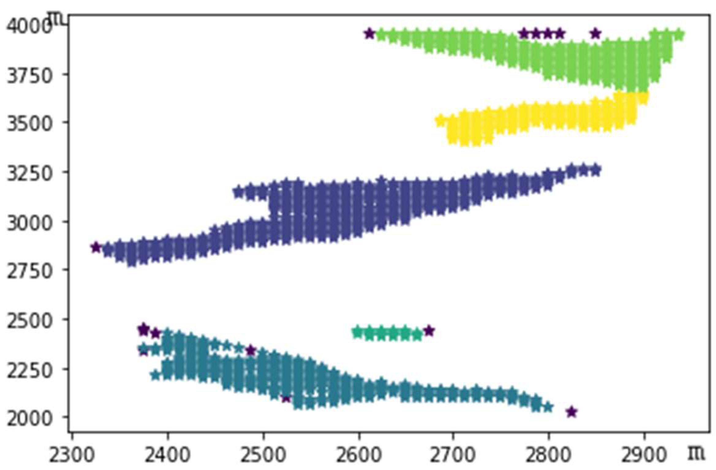
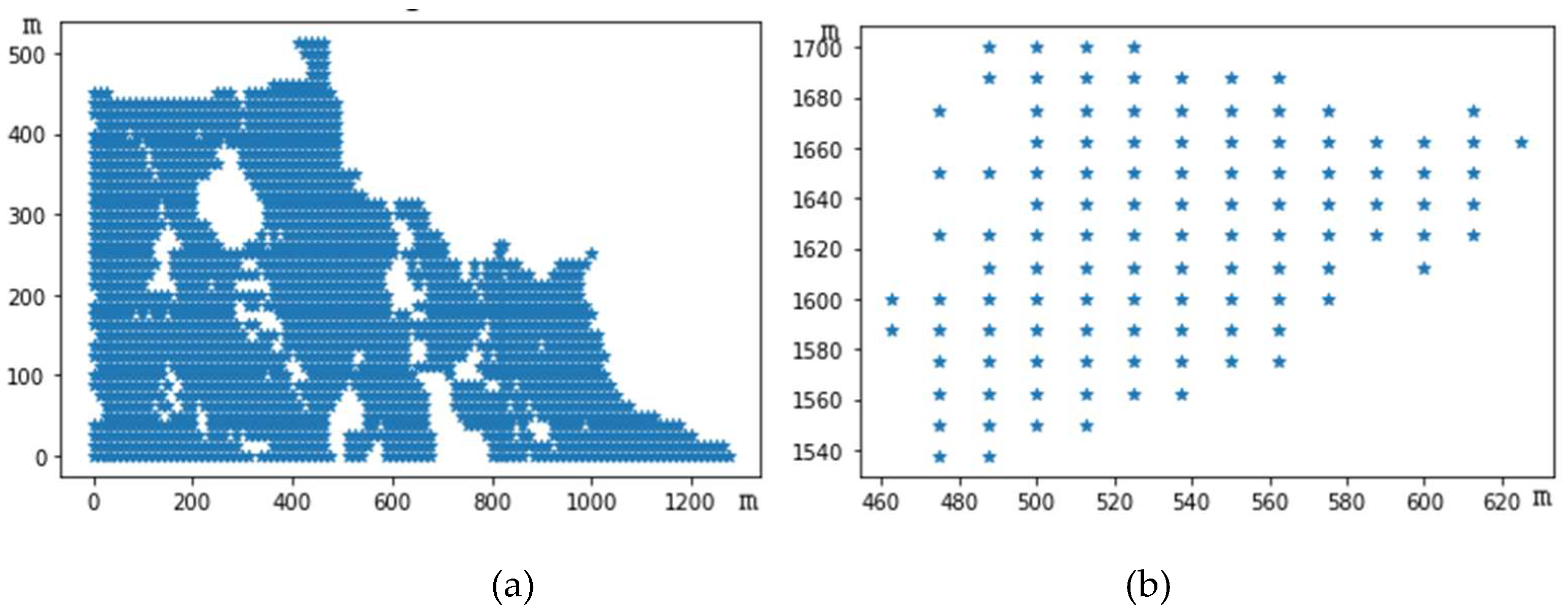
Consequently, clustering was executed with a minimum sample point count of 4 and a neighborhood radius of 18 meters, yielding the results depicted in
Figure 4.
The observation point is located at [2725, 2112.5, 334], with the longitude and latitude (118.845°E, 32.071°N) situated at a higher position on Purple Mountain, as shown in
Figure 1. A DBSCAN clustering analysis was conducted on the viewshed of the observation point, and the division after clustering is shown in
Figure 4. The entire viewshed is divided into five sub-viewsheds with 13 noise points.
Figure 4 displays the results of the division, where the coordinate axis uses the southwest edge of the map as the origin, with 12.5 meters as one grid precision, and relative coordinates represent the distance relationship between each sub-viewshed.
The overall distribution of the visible points is relatively uniform, with its essential distribution characteristics being that two sub-viewsheds are far apart or not adjacent. For points that are distributed adjacently and clustered together, it can be considered that the distance between the two points is less than or equal to the neighborhood radius value of 18 meters, and the number of sample points within the neighborhood range centered on a specific point reaches the minimum sample point number value of 4.
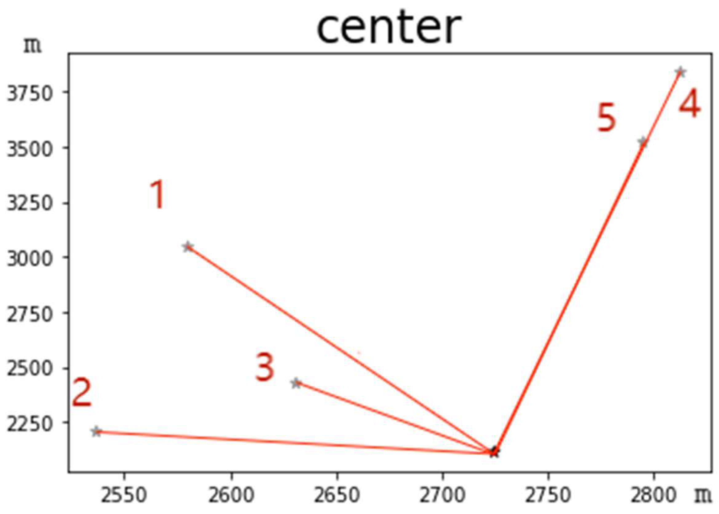
Constructing the spatial semantic relationship between sub-viewsheds and viewpoints reveals that sub-viewsheds are distributed in multiple viewing directions from the observation point. The direction and distance of each sub-viewshed from the viewpoint can be determined by calculating the azimuth attributes of the sub-viewsheds. The divided sub-viewsheds are labeled in
Figure 5 in the order of
Table 1 sub-viewshed numbers, the gray mark indicates the center point of each sub-viewshed, and the black mark indicates the observer point position. The abscissa and ordinate represent the relative distance between sub-viewsheds, starting from the origin position, considering the terrain accuracy, measured in meters. As can be seen from
Figure 5, the field of view is basically on one side of the observer. When the observer looks around, more viewsheds can be seen on the north side, with no visible areas in the opposite direction. The 3D simulated map of this terrain is shown in
Figure 7, where the observation point is on one side of the mountain ridge line, and the line of sight on the other side is blocked.
Table 1 displays the internal attributes of each sub-viewshed after partitioning, where the clustering partition has the highest number of visible points in sub-viewshed 1, followed by sub-viewshed 2, and the lowest number of views in sub-viewshed 3.
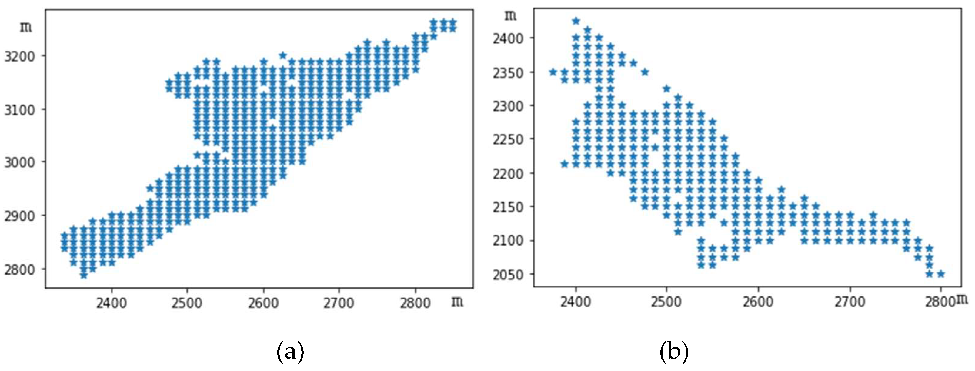
The shape of sub-viewshed 1 is shown in
Figure 6(a). There are 468 visible points within this sub-viewshed, with an area of 73,125 square meters and a density of 0.381. The distribution of visible points in this sub-viewshed is dense, indicating good view quality. The central point coordinates are [2580,3044], with an elevation value of 202.158 meters, situated at an intermediate altitude, and the visible points are distributed in the mountainside area. Sub-viewshed 1 is located at 99° from the observation point, approximately 952.081 meters from the observer. The distribution of visible points in the sub-viewshed is not concentrated enough, appearing linearly distributed. The average distance of the visible points is 200.36, and the sum of the central distances is 0.31. Due to the large number of visible points within the sub-area, the sum of the central distances is relatively small, and the lack of concentration in the distribution of visible points results in a more significant average distance of the view.
Sub-viewshed 2 contains 294 visible points, making it the second most populous area regarding the number of visible points. The shape is shown in
Figure 6(b). The average elevation of this sub-viewshed is 362.187 meters, which is at a relatively high altitude. The density of the sub-viewshed is 0.239. It is the closest view to the observer, approximately 211.691 meters away, located 154° from the observer. The horizontal distribution of visible points within the sub-viewshed spans considerably, with an average distance of 162.655. The sum of central distances is 0.4. Within the view range are areas without coverage by visible points, resulting in a relatively sparse distribution of visible points.
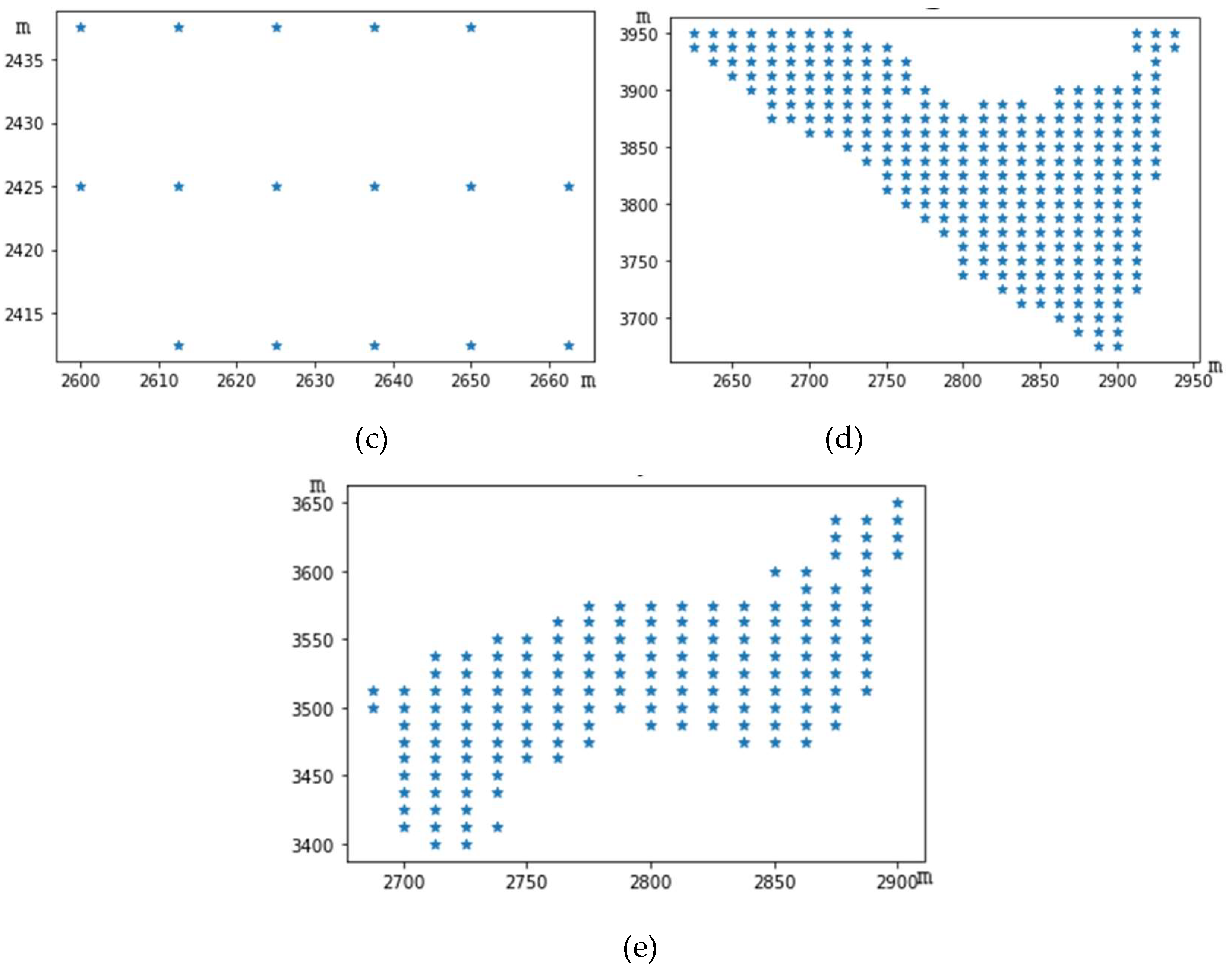
Sub-viewshed 3 has the most minor visible points, as shown in
Figure 6(c). The elevation of the center point of this viewshed is 286.562 meters, with 16 visible points. The viewshed is located 107° from the observation point, approximately 329.69 meters away, with an average distance of 27.428. This is the smallest average distance among all sub-viewsheds, and the sum of central distance is 1.277, which is the largest among all sub-viewsheds. Due to the small number of visible points in this sub-viewshed and their relatively concentrated distribution, each visible point is closely connected, forming a matrix-like distribution. This results in a situation where the average distance within the sub-viewshed is small while the sum of central distance is large.
The center of sub-viewshed 4 is located at [2813, 3838], with an average elevation of 84.425 meters, making it the lowest altitude among the five sub-viewsheds, as shown in
Figure 6(d). It has 275 visible points, a relatively high number distributed to this sub-viewshed, with a density of 0.224. This sub-view is the farthest from the observer at 1745.77 meters. The observer’s position is near the mountain top, while this sub-viewshed is located at the foot of the mountain. It is located at 87° of the observer. The shape distribution shows that the visible points are relatively concentrated, with an average distance of 132.128, and the sum of central distance is 0.351. Compared with sub-viewshed 2, it has fewer visible points but a smaller sum of central distance, indicating that the distribution of visible points in this viewshed is more concentrated and closer to the center than in sub-viewshed 2.
The elevation of Sub-viewshed 5 is 100.525 meters, which is the second lowest area compared to Sub-viewshed 4, as shown in
Figure 6(e). There are 160 visible points within this sub-viewshed, with a density of 0.13. Compared to the distribution of all visible areas, the number of viewpoints in this sub-viewshed could be sparser. According to the elevation, it is distributed at a lower altitude than the observation point. It is located at a distance of 1428.472 meters from the observation point, in the northeast direction by 87°. From
Table 1, it can be found that sub-viewsheds 4 and 5 are in the same direction as the observer; that is, when the observer looks in its northeast direction by 87°, they can simultaneously see the centers of sub-viewshed 4 and 5. The distance from these two sub-viewsheds to the observer is 1745.77 meters and 1428.472 meters. Since these three points are distributed on a straight line, it can be calculated that the center point distance between Sub-viewshed 4 and 5 is 317.298 meters, with an average distance of 101.837 meters, and the sum of the central distances is 0.465.
It can be observed that there are gentle terrains within each sub-viewshed, which is consistent with the characteristics of hilly terrains. The terrain does not fluctuate significantly and has a relatively mild slope. Purple Mountain, as a tourist attraction, has also been planned with multiple hiking routes for tourists to choose from, such as routes with steeper slopes and shorter durations, as well as routes with gentler slopes and longer durations. Except for Sub-viewshed 3, the average distances in the other sub-viewsheds are relatively large for two reasons: firstly, the visible points in the sub-viewshed are not concentrated, resulting in more considerable distances between two points; secondly, the number of visible points in the sub-viewshed is small. Compared with sub-viewshed 1 and 2, sub-viewshed 1 has a more significant number of visible points, differing by 174, but the difference in average distance is relatively small, about 38. This is due to the distribution of visible points in the sub-viewshed needing to be more concentrated, leading to more considerable distances between two visible points and thus increasing the average distance. From the shape distribution of these five sub-viewsheds, the distribution of visible points is relatively scattered and not concentrated enough, resulting in a larger average distance. At the same time, the sum of central distances is also an indicator reflecting the degree of concentration of visible points. The closer the distribution of visible points is to the center position, the smaller its value. Although sub-viewshed 1 has a more significant average distance, its maximum number of visible points results in a smaller sum of central distances; sub-viewshed 3, due to its smaller number of visible points, has a more enormous sum of central distances than the others.
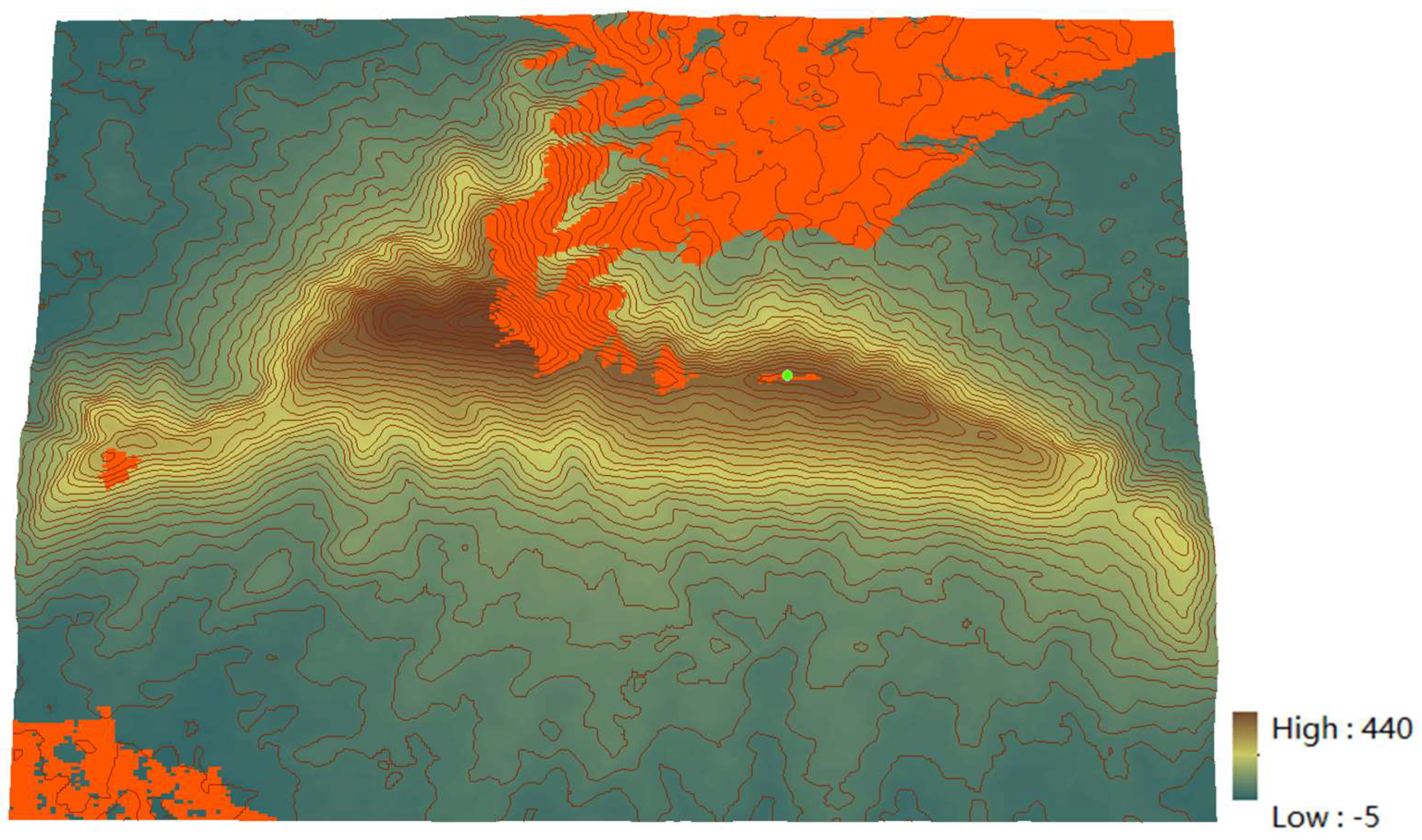
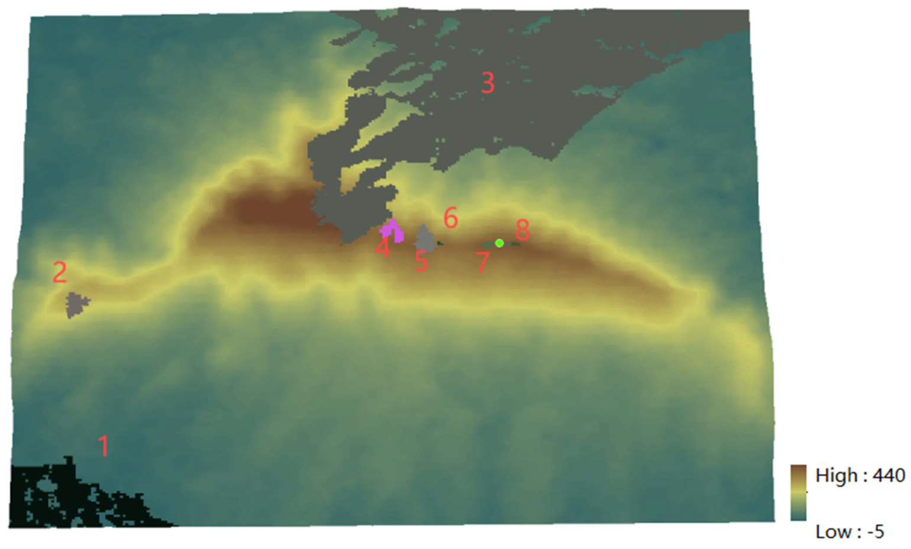
Observing from two different positions north and south of Purple Mountain, the three-dimensional display of the viewshed division results is shown in
Figure 7,
Figure 7(a) is a view of the south side of the Purple Mountain, and
Figure 7(b) is a view of the north side of the Purple Mountain. Sub-viewshed 2 is distributed in the high-altitude area close to the mountain ridge line, and this viewshed has a wide range of visible points. Sub-viewshed 3 is located at the mountainside, which is also in a high-altitude area, but its elevation is lower than that of sub-viewshed 2, yet higher than sub-viewsheds 1, 4, and 5. Sub-viewshed 4 has the lowest altitude, near the foot of the mountain. Overall, sub-viewsheds 1, 4, and 5 are situated at relatively lower altitudes, with the region relatively flat.
Figure 7.
Three-Dimensional Diagram of Viewshed Partitioning.
Figure 7.
Three-Dimensional Diagram of Viewshed Partitioning.
A new target point for observation is selected to perform viewshed analysis at this location. The resulting viewshed is depicted in
Figure 8. The observer’s coordinates are (118.855°E, 32.07°N) with an elevation value of 356 meters near the ridge line. A more extensive area is visible on one side of the ridge, demonstrating a broad field of view coverage distribution. Conversely, only a smaller area is observable on the other side of the hill.
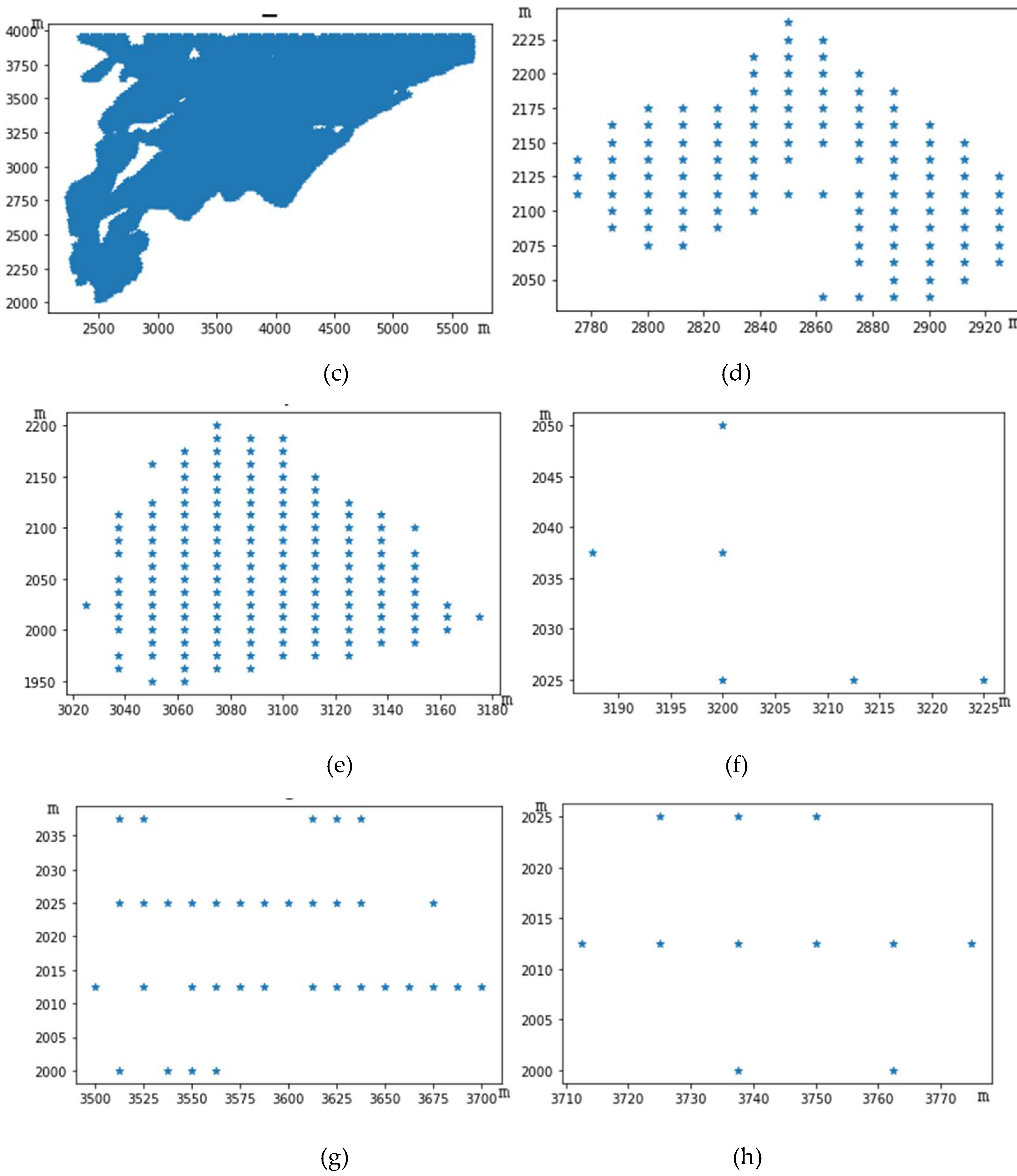
Cluster analysis is performed on the terrain elevation within the range encompassed by the viewshed. Under the proposed methodology, suitable parameters are chosen for clustering. The viewshed is segmented into eight distinct sub-viewsheds, as
Figure 9(a) depicts.
Figure 9(a) highlights a notable disparity in the number of visible points, where each sub-viewshed encompasses within the viewshed partition.
Figure 9(b) delineates the spatial relationship between the center of each sub-viewshed and the observation point. The results of attribute value calculations within the sub-viewshed are presented in
Table 2. Sub-viewshed 3 boasts the highest count of visible points, averaging an elevation of 103.687 meters. This is higher than that of sub-viewshed 1 but lower than others. This discrepancy can be attributed to the relatively flat terrain slope in this region, which lacks any steep inclines, leading to a concentration of more visible points totaling 17961. The density of the sub-viewshed is 0.8752, making it the sub-viewshed with the most visible points and the largest proportion among all visible points, yielding the best field of view quality. Sub-viewshed 3 is situated 89° from the observer at 1317.525 meters. This sub-viewshed encompasses a broad range. Due to the large number of visible points within sub-viewshed 3, the distribution of visible points in the area extends outward on both sides, resulting in the largest diameter involved and causing the maximum average distance within the sub-viewshed, which is 1144.833. Given many visible points in sub-viewshed 3, its sum of center distance is the smallest among all sub-viewsheds.
Sub-viewshed 1 is situated at the relative coordinate [457,188], as depicted in
Figure 10(a). The average elevation of sub-viewshed 1 stands at 25.098 meters, making it the lowest among all sub-viewsheds. The average elevation of visible points within this sub-viewshed is notably low, and the number of discernible grid points is relatively high. This suggests that sub-viewshed 1 is likely located in a predominantly flat area. Within its viewshed are 2112 visible points, ensuring a broad visual range. Sub-viewshed 1 is positioned 210° from the observer, at 3676.195 meters, making it the observer’s most distant viewshed. As illustrated in
Figure 8, sub-viewshed 1 is situated in a lower altitude corner area near the mountain’s base. At the same time, the observer is located near the ridge line at a higher altitude, resulting in a greater distance between them. The average distance of Sub-viewshed 1 is 409.653, indicating that the distribution of this viewshed is not sufficiently clustered. The distribution of visible points is either horizontal or vertical, failing to form a circular shape, which leads to larger attribute values.
The elevation of Sub-viewshed 2 is 230.628 meters, as shown in
Figure 10(b). As can be seen from
Figure 8, it is located at a relatively high altitude within the Purple Mountain branch hill, with 113 visible points in the viewshed, 3121.113 meters away from the observer, and 7° southwest of the observer. The average distance of sub-viewshed 2 is 76.167, and the sum of central distances is 0.494.
Sub-viewshed 4 is located at [2855,2128], as shown in
Figure 10(d). The elevation value of the sub-viewshed is 322.147 meters, with a total of 116 visible points and a density of 0.0057. The number of visible points is like that of sub-viewshed 2. It is 776.723 meters from the observation point and 8° northwest of the observer. The average distance of the sub-viewshed is 82.174, and the sum of central distances is 0.523. Compared with Sub-viewshed 2, these two sub-viewsheds have a similar number of visible points, both on the western side of the observer’s viewpoint, but differ in shape distribution. The difference between their average distance and the sum of central distance is not significant, indicating overall similarity in attribute values between the two sub-viewsheds.
From the perspective of directional attributes in sub-viewsheds, sub-viewsheds 4, 5, 6, and 7 are within a specific fixed visual range of the observer, and the distances between these sub-viewsheds are not far. When the observer looks in a specific direction, they can see these four sub-viewsheds simultaneously. Sub-viewshed 5 is located 4° northwest of the observer, at 535.664 meters; sub-viewshed 6 is located 1° northwest of the observer, at 421.76 meters; sub-viewshed 7 is located 10° southwest of the observer, at a distance of 36.363 meters, which is also the closest sub-viewshed to the observer. To the observer, the visual angles of these sub-viewsheds form an angle of 18 degrees. With attention concentrated, the human eyes’ visible field of view is approximately 25 degrees. Therefore, when viewing from a certain angle, the observer can focus their attention and simultaneously see these four sub-viewsheds. Although sub-viewshed 2 is also within this visual angle range, due to its great distance, the visual effect of sub-viewshed 2 will decrease when the observer is looking closely.
The shape of each sub-viewshed division is shown in
Figure 10. The sub-viewshed with the highest number of visible points is sub-viewshed 3, while the one with the least number of visible points is sub-viewshed 6, which has only 6 visible points. This sub-viewshed is at a higher altitude, with an elevation value of 329.334 meters. The distribution of visible points is shown in
Figure 10(f). As can be seen from the figure, the visible points are distributed within a 3×4 grid unit, and this viewpoint is near the ridge line of Purple Mountain, where there exists flat land within the viewpoint.
The results reflected from the internal attribute values suggest that the distribution of visible points in sub-viewsheds 7 and 8 is relatively similar. The elevation values of these two sub-viewsheds differ slightly, with the number of visible points in sub-viewshed 7 being approximately three times that of sub-viewshed 8. This is also reflected in the average distance attributes, which are nearly three times as much. Due to the more significant number of visible points in sub-viewshed 7, the sum of central distance is slightly smaller compared to sub-viewshed 8. As can be seen from
Figure 10, both sub-viewsheds 7 and 8 exhibit a horizontal stripe distribution.
The average distance attributes of sub-viewshed 2 and 7 differ slightly, but sub-viewshed 2 has 113 visible points, while sub-viewshed 7 has only 35. This difference in the number of visible points is due to the distribution of visible points in the two sub-viewsheds. The distribution of visible points in sub-viewshed 2 is more concentrated, resulting in a smaller distance between any two visible points within the view. On the other hand, the distribution of visible points in sub-viewshed 7 is linear, with no concentration, leading to a large distance between any two points within the view. This results in a slight difference in the average distances between the two sub-viewsheds. It also reflects that the distribution of sub-viewshed 7 is sparser than that of sub-viewshed 2, with a more concentrated distribution of visible points in sub-viewshed 2.
Figure 11 shows the three-dimensional graph of terrain after clustering partition. The figure shows that the visible points in sub-viewshed 3 involve a larger area, from the bottom of the mountain to the slope and finally to the ridge line position. The distance between any two adjacent visible points within this sub-viewshed is less than or equal to 18 meters; thus, they are clustered together. This feature also reflects the relatively flat characteristics of the terrain in this sub-viewshed. Based on this sub-viewshed, path planning for mountain climbing roads can be conducted so that tourists will not walk to steep slopes during their ascent.
The observation point is located on the north side of the ridge line, allowing it to see a larger area on one side. In contrast, the other side is not fully visible due to obstructions in the line of sight, and only a tiny part of the distance can be seen. The figure shows that sub-viewsheds 4, 5, 6, 7, and 8 are distributed along the ridge line. A walking path can be planned based on these sub-fields for tourists to enjoy. If the position of the observation point is set as an observation post or target scenic area, all sub-viewsheds can simultaneously see this target point.