
Submitted:
18 January 2025
Posted:
20 January 2025
You are already at the latest version
Abstract
Synthetic Aperture Radar provides high-resolution imaging independent of 1 weather conditions. SAR data is acquired by an aircraft or satellite and sent to a ground 2 station to be processed. For novel applications requiring on-time processing for real-time 3 analysis and decisions, onboard processing is necessary to avoid the limited down-link ca- 4 pacity and reduce data analysis latency for real-time decisions. Real-time target recognition 5 from SAR data has emerged as an important task in many areas, like defense and surveil- 6 lance where targets must be identified as fast as possible. The accuracy of target recognition 7 algorithms has improved by applying deep learning models. These are computationally 8 and memory expensive, which requires optimized models and architectures for efficient 9 deployment in onboard computers. This paper presents a fast and accurate target recogni- 10 tion system directly on raw SAR data. The neural network model receives and processes 11 SAR echo data for fast processing, without computationally expensive DSP image genera- 12 tion algorithms such as BackProjection and RangeDoppler. This permits the utilization of 13 simpler and faster models, but still very accurate. The system was designed, optimized, 14 and tested on low-cost embedded devices with low energy requirements, namely a Khadas 15 VIM3 and a Raspberry Pi 5.The solution achieves a target classification accuracy for the 16 Moving and Stationary Target Acquisition and Recognition (MSTAR) dataset close to 100% 17 in less than 1.5 ms and 5.5W of power.
Keywords:
SAR echo data
; Target Recognition
; Neural Network
; Embedded System
1. Introduction
Synthetic Aperture Radar (SAR) technology is widely used for many applications that require the identification of planet surface objects and scenarios in any weather condition, such as tracking ships and oil spills, terrain erosion, drought and landslides, deforestation and fires [1]. There have been works that focused on SAR image classification for such applications using deep learning. Most works first process the captured SAR echo data into an image and then apply deep learning models to classify the objects. This processing flow requires the execution of an image reconstruction algorithm and the inference of a deep learning model for classification. Given the complexity of SAR image formation algorithms [2] and of accurate deep learning models for image classification, this approach is computationally expensive and, therefore, may be infeasible for time-sensitive applications such as defense and surveillance. Furthermore, each task in the processing flow introduces errors that accumulate after the complete processing, reducing the precision of the classification.
Using a neural network to recognize targets directly from the SAR echo data alone would allow object classification without the need to process the data into an image, an often time-consuming operation, as well as reduce the source of errors. In theory, raw data classification should achieve results with higher accuracy than the classification of SAR images after image formation because the final image lacks the details still present in the data before processing.
In SAR Automatic Target Recognition (ATR), situations where the captured target configuration differs from the training data configuration can considerably degrade the accuracy of the results. These conditions are referred to as Extended Operation Conditions (EOC) [3]. Situations where the target configuration is closer to matching the data on which the network was trained are referred to as Standard Operation Conditions (SOC). In this work, both conditions were considered to show the robustness of the proposal.
The Neural network models to be executed onboard must be carefully designed to avoid high computing requirements and energy consumption. So, the structure of the proposed neural network model was found through a design model exploration and mapped to an embedded low-cost yet powerful device for low energy consumption.
This work proposes an optimized neural network to classify targets captured by SAR directly from the SAR echo data. A simple yet effective neural network is explored and tested to classify SAR echo data. The proposed network is robust enough to classify both SOC and EOC with extreme accuracy. It can classify data from the MSTAR dataset [4] with accuracies above 99% in both SOC and EOC. The neural network was optimized and implemented on two single board computers, Khadas VIM3 and Raspberry Pi 5 due to their small Size, Weight and Power (SWaP) constraints. It was also tested in embedded devices, specifically a Khadas VIM3 and a Raspberry Pi 5, for potential on-the-go ATR on the SAR equipped platform.
2. Related Work
Early machine learning algorithms for the classification of objects from SAR images focused on identifying features such as geometric features [5], histogram of oriented gradient [6], fusion features [7], scattering features [8] and statistical features [9], among others.
Recently, with the advent of deep learning, these features are automatically learned, achieving better performance. Object classification applied to SAR has been proposed as a means to extract information from captured scenes to aid in quicker and/or automated decision-making. Some works focus on target classification based on SAR images. The work in [10] was one of the first approaches to consider Convolutional Neural Network (CNN) for SAR image classification. They propose all-convolutional network (A-ConvNet), a network with sparse layers to reduce the overfitting problem. They also established the configuration for SOC and EOC in most future classification works that also use MSTAR [4]. SOC imply training with data that was captured at a 17º depression angle and testing with 15º depresson angle data. EOC implies training with the same type of data but testing with 30º depression angle data. Any mention of SOC and EOC throughout this article refers to these conditions unless stated otherwise. The network achieved an accuracy of 99.13% for SOC 87.40% for EOC. The work also explores the introduction of random noise in the input data observing a large impact on the accuracy.
To deal with scarce SAR data, CHU-Net [11], a CNN network with dropout to avoid overfitting from scarce data, was proposed to classify SAR images. When using all data, the model achieves an accuracy close to 99%, which drops to 94% when trained with a small subset of the training data.
Another work looking for a solution to scarce data [12] proposes Amplitude-Phase cnn (AP-CNN), a CNN that considers both amplitude and phase of SAR data. This improves the accuracy of the algorithm in EOC when trained with scarce data compared to methods that only consider the amplitude. The CNN achieved accuracies of 98.10% and 93.57% in SOC and EOC, respectively. A two-step approach was considered in [13] to deal with lack of training data. An initial step uses a CNN to extract features to train a second CNN for SAR image classification.
Hybrid models were also considered for target classification of SAR images. Some consider the integration of two types of deep learning models such as [14] where a CNN is combined with a Long Short-Term Memory (LSTM) model. A CNN is used to extract features, enhanced with a spatial attention module, followed by LSTM that fuse features from adjacent azimuths when multiview images are present. This network achieved accuracies of 99.38% and 95.57% in SOC and EOC, respectively. Other hybrid approaches consider a deep learning model combined with traditional machine learning algorithms. In [15], a histogram-oriented gradient is combined with a CNN enhanced with the attention mechanism. Two SAR ship datasets are tested: OpenSARShip [16] and FUSAR-Ship [17]. Their network, HOG-ShipCLSNet, achieved accuracies of 78.15% and 86.69% with each dataset, respectively.
In [18], data augmentation techniques such as clutter transfer are applied to images in the MSTAR dataset [4] to improve the robustness of target recognition, with a specially tuned ResNet18 network. The work achieves an accuracy of 97.2%. With non-ideal ResNet18 parameters and contrast balancing, it achieved an average accuracy of 88.5%. It also considered experiments with changing the background clutter and generating synthetic images, with a minor impact on the accuracy.
Transformers and attention mechanisms are at the core of the most recent SAR image classifiers [19,20,21]. One of the most recent works [21] achieves accuracies of up to 99.79% in SOC and up to 98.52% in EOC on MSTAR [4]. The work also achieves an approximate accuracy of 84.25% throughout the different versions of the OpenSARShip [16] dataset.
Deep learning-based methods are effective in identifying ships in SAR images. However, echo data has to be preprocessed with correction functions, and converted to an image, which is finally processed with a target detection algorithm. Transmission of echo data should be included in the processing flow if data is processed in a ground station. For real-time target detection onboard, the computational and energy onboard requirements are high. Taking this into account, a new research direction was taken focused on ATR directly applied to the raw SAR data.
Recent works [22] and [23] focused on ATR with raw Ground-based Synthetic Aperture Radar (GBSAR) data. GBSAR is a variation of SAR that is typically applied in indoor environments. These articles use a custom-made sensor attached to a rail to capture small objects of different shapes and materials. In [22], a modified ResNet18 network was trained to perform multilabel classification on three bottles of varying material. Various experiments were conducted, such as different weight initializations, and comparing raw data and image classification results. Raw data classification achieved the best results with a mean F1 score of 88.24%. In [23], the same modified ResNet18 was used to train on GBSAR data with different polarizations mixed into the input in different ways, such as mixing the rows of data or appending horizontal polarity data to vertical polarity data, referred to as JOIN. The previously mentioned article only used data with horizontal polarization. This article also created a siamese model that combined the results of two separate ResNets, trained on each polarization. The JOIN model resulted in the highest accuracy, which was 93.06%.
Fast Range-Compressed Detection (FastRCDet) was proposed in [24], a novel lightweight network for ship detection that accepts range-compressed SAR echo data as its input. The network was conceived to detect ships onboard the SAR platform. They also propose a network to adapt the data to the range-compressed domain. The lightweight network with 2.49M parameters is able to detect ships with an average accuracy of 77.12%.
SAR image classification works achieve accuracies around 99% but requires a SAR image formation step and complex CNN models. Works on SAR echo data classification are still in their infancy but the results are promising. The work proposed in this paper contributes to ATR on raw SAR echo data. An optimized neural model is designed to achieve high accuracy, avoid overfitting due to scarce data, and reduce memory and computing complexities for onboard execution at low energy.
3. Neural Network Architecture
The main goal of this work was to define the smallest and simplest possible neural network architecture that could produce highly accurate SAR classification results. All networks sizes that were tested had the base architecture shown in Figure 1. Each hidden layer is dense and uses ReLU as the activation function. In this diagram, i corresponds to the number of input neurons, k corresponds to the number of output neurons, and j is the number of neurons in the first hidden layer. The number of outputs depends on the conditions the network is for: SOC or EOC. The k-value depends on the dataset used and corresponds to the output classes. The j-value is the main focus of the network size experiments. Values between 60 and 20 were tested. By default, the i-value is the size of a raw echo data sample in the dataset being used. The network expects magnitude data as an input.
3.1. MSTAR Dataset
The MSTAR dataset [4] is widely used for SAR ATR tasks. It contains labeled raw data and images of various armored vehicles. The dataset also contains data captured in different conditions, mainly different depression angles. It was chosen for its availability and popularity.
The most abundant data present in the dataset had a depression angle of 17º. This data included 7 classes with 300 samples each: 2S1, BRDM_2, D7, SLICY, T62, ZIL131, and ZSU_23_4. This data was therefore determined for training. Data with a depression angle of 15º was divided into the same 7 classes, but only contained 274 samples each. Since 15º and 17º depression angles are similar, 15º depression angle data was used for testing the network in SOC. There were only 4 classes that had data with a 30º depression angle: 2S1, BRDM_2, SLICY, and ZSU_23_4. This extreme angle was chosen for training the proposed networks in EOC.
Inspired by [10], the data with varying depression angles was used to test the robustness of the proposed network. In SOC, 17º data was used to train the network on all 7 classes and 15º data was used to test. EOC refers to the conditions in which a target can be captured that are outside the expected, leading to lower accuracy ATR results [25]. In this case, MSTAR data captured with a depression angle of 30º was used for testing a network trained in 17º angle data to see how the network classified these extreme conditions.
3.2. Varying Sizes of Raw Data
An initial problem was identified with the data present in the dataset: the size of the samples varied between classes. The input size of the network must remain constant. In image classification tasks, it is common to resize the image to 224x224, not only to make the input size constant but also to reduce the processing times of training and inference. However, raw data should not be treated like an image. The chosen solution was to create a range of the data that had to at least contain the target (typically the center of the signal or, after image processing, the center of the image). This range of data is referred to as a “window”. Signals shorter than the window’s size were given 0 padding, while signals that were longer were cut.
Two of the classes, 2S1 and ZSU_23_4, had approximately the same size of 25000 data values. The window was therefore defined as having a range of 0-25000. The other classes were verified to confirm that a window of such a range did not cut off the target, which is the object to classify. If there are ever other datasets that share this size problem, the same method can be applied. Otherwise, in datasets with consistent raw data sample sizes, the window serves only in the case described in the following subsection.
3.3. Network Size Reduction
The first experiment to shorten the input size involved reducing the size of the input data by altering the start and length of the data window. The window reductions have a limit, as they must contain the most important part of the signal: the target. As an example for the MSTAR dataset, a window region of 1000-20000 was determined to be suitable for all classes. This results in an input size of 19000, a reduction in 6000 data values. Figure 2 displays plots of raw data from randomly selected samples of 6 classes. It also contains a square drawn in each plot corresponding to the window region of 1000-20000. The peaks in the middle of each signal correspond to the targets. SLICY, the class with the shortest samples, has a target that barely fits in the defined window interval. ZIL131, the class with the longest samples, seems to have a part of the target outside the range. Based on later results, this is not a problem, as enough characteristics can be extrapolated from the target data inside the window.
The sampling of the input data is another aspect that was explored. This process consists of using only every Nth data value of the input, effectively reducing its size. Multiples of two between 2 and 8 were tested. In the MSTAR dataset’s case, with the shortened window size and sampling with N>1, the input size varied between 10000 and 2500.
4. Results
All generated network models were trained using categorical cross-entropy as the loss function, Adam as the optimizer, a learning rate of 0.001, a batch size of 32, and 10 epochs. The learning rate and number of epochs were chosen to match the size of the data, which is small compared to the usual 224x224 image in image classification tasks.
The MSTAR dataset was used to experiment on the size of the network. A public tool called “mstar2raw” was used to separate the magnitude data from the full raw data samples. This data was then converted to csv files.
4.1. Standard Operation Conditions
The SOC accuracy results were tested for different sizes of the architecture. The 17º depression angle data was split into training and validation groups (80/20) and the 15º depression angle data, present in the same dataset, was used to test. Table 1 shows the accuracy of each attempted network. The Layer 1 and Layer 2 columns show the number of neurons in the respective hidden layers of the network. The table shows smaller networks perform better. This could be due to the size of the small dataset compared to the larger networks. However, the accuracy result differences are extremely small, so they are most likely the result of a margin of error.
The experiments ended with a network with 20 neurons on the first layer and 10 on the second layer. This stopping point was chosen because far worse accuracy results were expected to occur for very small networks, especially after the reduction steps mentioned in SubSection 3.3, which are further explored in the following subsection.
4.1.1. Reducing the Input Data Size
This network is very simple, but the size of the input data implies a high number of parameters since the input size is 25000 and the input is fully connected to the neurons of the first hidden layer. The window size reduction described in Section 3 is applied in the following experiments.
The results of the window size reduction can be seen in Table 2.
As can be observed from the results in the table, the model size can be reduced to one third with a neglegible degradation in accuracy.
4.2. Extended Operation Conditions
Unlike the 17º and 15º depression angle data, MSTAR only contained 4 classes of 30º angle data: 2S1, BRDM_2, SLICY, and ZSU_23_4. Due to this lower number of classes, the network was trained with the respective classes in 17º depression angles. Similarly to the previous experiments in SOC, several networks were trained to determine how small the network could be before noticeable drops in accuracy could be observed. The 30º angle data was also used as the validation group to observe drops in accuracy. Like in SOC, the initial experiments were performed with a window size of 0-25000 and a sampling of 1. The results can be seen in Table 4. The network sizes are the same as in SOC, Table 1, so those columns were omitted. However, due to the difference in conditions between the training data and the testing data, the accuracy fluctuates more than in SOC. Therefore, new columns were added that display the final and best accuracies of the network, along with the epoch in which it achieved the best accuracy.
The results show a great decrease in average accuracy starting in the network architecture which has 30 neurons in the first layer. Therefore, the one with 40 neurons in that layer was selected for further experimentation. Table 5 shows the results of this network with a window size of 1000-25000 and a varying sampling number. The network sizes are present in the table for ease of access.
4.3. Comparing Results to Related Works
In SOC, the smallest tested network still manages to achieve an accuracy of 99.896%. Therefore, the proposed network for SOC is the network with 20 neurons in the first hidden layer, 10 neurons in the second layer, a window size of 1000-20000 on the input data, and a data sampling of N=8.
In EOC, a small decrease in precision was observed in the smallest tested networks. The proposed network for EOC has 40 neurons, a window size of 1000-20000, and a data sampling of N=4. This was chosen for its accuracy and reduced size. The network with 50 neurons in the first layer shares the same best accuracy but is larger. The best accuracy was observed in the 6th epoch at 99.48% before decreasing to 98.87% by the 10th epoch.
None of the related works are reported to reach accuracies this high. Yoon et al. [21] report values that come close, with 99.79% on SOC and 98.52% on EOC. However, an input image requires the raw data to be processed into an image first, which implies a more power-consuming and time-consuming “pre-processing” step.
From the related works that use raw data as input, the highest accuracy achieved was 93.06% on GBSAR using a modified ResNet. A common thread in these works is the use of deep neural network architectures commonly applied to image classification tasks on raw SAR data. According to our results, simple fully connected neural networks can be trained to achieve even higher target classification accuracy, even in EOC. Table 6 compares the results of the proposed networks with other networks from related works. The highest accuracies in each category (images and raw data) for each set of conditions, SOC and EOC, are in bold.
4.4. Embedded Device Implementation
The proposed networks were first implemented on a desktop computer with an AMD Ryzen 9 7900X3D Central Processing Unit (CPU) with 12 cores, 64GB of RAM and an Nvidia GeForce RTX 4080 running CUDA 12.0. To test their effectiveness in more limited conditions, the networks were also implemented on a variety of embedded devices to compare each of their inference speeds and power consumption. All network implementations were performed in Python. The tested devices were Khadas VIM3 and a Rapsberry Pi 5. The Khadas possesses a quad-core ARM Cortex-A73 CPU running at 2.2GHz and the Rapsberry Pi has a quad-core ARM Cortex-A76 CPU running at 2.4GHz. Table 7 shows these metrics. The reported power consumption corresponds to the highest wattage observed during inference. Inference times were measured while inferring with batches of 32 raw data samples. EOC have longer inference time due to the larger size of the network proposed for these conditions. The difference in power consumption between the NVIDIA Graphics Processing Unit (GPU) and the embedded devices highlights the different applications of such devices, as a flying SAR equipped platform would not be able to host said GPU effectively. The GPU would require too much power. Still, the device is reported here to compare inference times with related works.
Some of the related works provided inference time metrics as well. These metrics would commonly be displayed in FPS, so they were converted to milliseconds for comparison purposes. Table 8 compares the results between related works. Only Yoon et al. [21] showed the results for the different conditions. The proposed network of Yoon et al. [21], besides having the highest accuracy when compared to other related works, also reports the quickest inference times. However, the network is slower than the network proposed in this article, which was executed on an inferior GPU (RTX 4080 vs. RTX 4090).
5. Discussion
The results of the proposed small neural networks were unexpected but welcome. The work demonstrates that with a small network, it is possible to achieve accurate target detection on low-power embedded systems that can run onboard in real-time. Even data with a widely different depression angle was classified with stunning accuracy. Compared to previous works that classify SAR images after image formation, the proposed work achieves better accuracies and can run on low-power embedded devices, while image-based detection must run on high-power devices to achieve the same processing times.
The size of input data can be further reduced by removing background noise and only feeding target data to the network. Despite the target range of each class being different, a static window range was chosen for consistency. However, there is potential in having an even smaller window if the start of the window is aligned with the start of the target range of each class. This reduction has a large impact on the dimension of the neural network since most parameters of the model are relative to the connections neurons of the input layer and the first hidden layer.
6. Conclusions
A small neural network has been proposed for onboard target detection directly from SAR echo data. This avoids the utilization of costly SAR image formation algorithm and allows its efficient execution onboard with low-pwoer.
As the results show, the proposed network for SOC, the smallest tested network, can achieve extremely high accuracies as high as 99.896%. EOC call for a slightly larger network, to achieve accuracies of 99.48%. The proposed networks outperform current state-of-the-art alternatives, as demonstrated by the high-accuracy results. In addition, the sizes of the proposed networks make them energy and resource-efficient, facilitating their implementation in embedded devices for installation on the moving SAR platform.
Author Contributions
For research articles with several authors, a short paragraph specifying their individual contributions must be provided. The following statements should be used “Conceptualization, G.J. and R.P.D.; methodology, G.J. and M. V.; software, G.J.; validation, G.J., M.V. and P.F.; investigation, G.J.; writing—original draft preparation, G.J.; writing—review and editing, G.J. and M. V.; supervision, R.P.D., M. V. and P.F; project administration, R.P.D.; funding acquisition, R.P.D. All authors have read and agreed to the published version of the manuscript.
Funding
This work was supported by national funds through Fundação para a Ciência e a Tecnologia (FCT) with references 2023.15325.PEX
Data Availability Statement
This work used the following publicly available dataset: MSTAR Dataset (https://www.sdms.afrl.af.mil/index.php?collection=mstar).
Conflicts of Interest
The authors declare no conflicts of interest.
References
- Trinder, J.C. Editorial for Special Issue “Applications of Synthetic Aperture Radar (SAR) for Land Cover Analysis”. Remote Sensing 2020, 12. [Google Scholar] [CrossRef]
- Cruz, H.; Véstias, M.; Monteiro, J.; Neto, H.; Duarte, R.P. A Review of Synthetic-Aperture Radar Image Formation Algorithms and Implementations: A Computational Perspective. Remote Sensing 2022, 14. [Google Scholar] [CrossRef]
- Keydel, E.R.; Lee, S.W.; Moore, J.T. MSTAR extended operating conditions: a tutorial. In Proceedings of the Algorithms for Synthetic Aperture Radar Imagery III; Zelnio, E.G.; Douglass, R.J., Eds. SPIE, 1996. [CrossRef]
- Laboratory, S.N. Moving and Stationary Target Acquisition and Recognition (MSTAR) Dataset, 2005.
- Lang, H.; Wu, S. Ship Classification in Moderate-Resolution SAR Image by Naive Geometric Features-Combined Multiple Kernel Learning. IEEE Geoscience and Remote Sensing Letters 2017, 14, 1765–1769. [Google Scholar] [CrossRef]
- Lin, H.; Song, S.; Yang, J. Ship Classification Based on MSHOG Feature and Task-Driven Dictionary Learning with Structured Incoherent Constraints in SAR Images. Remote Sensing 2018, 10. [Google Scholar] [CrossRef]
- Zhou, G.; Zhang, G.; Xue, B. A Maximum-Information-Minimum-Redundancy-Based Feature Fusion Framework for Ship Classification in Moderate-Resolution SAR Image. Sensors 2021, 21. [Google Scholar] [CrossRef] [PubMed]
- Wang, X.; Liu, C.; Li, Z.; Ji, X.; Zhang, X. Superstructure scattering features and their application in high-resolution SAR ship classification. Journal of Applied Remote Sensing 2022, 16, 036507. [Google Scholar] [CrossRef]
- Wu, F.; Wang, C.; Jiang, S.; Zhang, H.; Zhang, B. Classification of Vessels in Single-Pol COSMO-SkyMed Images Based on Statistical and Structural Features. Remote Sensing 2015, 7, 5511–5533. [Google Scholar] [CrossRef]
- Chen, S.; Wang, H.; Xu, F.; Jin, Y.Q. Target Classification Using the Deep Convolutional Networks for SAR Images. IEEE Transactions on Geoscience and Remote Sensing 2016, 54, 4806–4817. [Google Scholar] [CrossRef]
- Lin, Z.; Ji, K.; Kang, M.; Leng, X.; Zou, H. Deep Convolutional Highway Unit Network for SAR Target Classification With Limited Labeled Training Data. IEEE Geoscience and Remote Sensing Letters 2017, 14, 1091–1095. [Google Scholar] [CrossRef]
- Deng, J.; Bi, H.; Zhang, J.; Liu, Z.; Yu, L. Amplitude-Phase CNN-Based SAR Target Classification via Complex-Valued Sparse Image. IEEE Journal of Selected Topics in Applied Earth Observations and Remote Sensing 2022, 15, 5214–5221. [Google Scholar] [CrossRef]
- Huang, Z.; Yao, X.; Liu, Y.; Dumitru, C.O.; Datcu, M.; Han, J. Physically explainable CNN for SAR image classification. ISPRS Journal of Photogrammetry and Remote Sensing 2022, 190, 25–37. [Google Scholar] [CrossRef]
- Wang, C.; Liu, X.; Pei, J.; Huang, Y.; Zhang, Y.; Yang, J. Multiview Attention CNN-LSTM Network for SAR Automatic Target Recognition. IEEE Journal of Selected Topics in Applied Earth Observations and Remote Sensing 2021, 14, 12504–12513. [Google Scholar] [CrossRef]
- Zhang, T.; Zhang, X.; Ke, X.; Liu, C.; Xu, X.; Zhan, X.; Wang, C.; Ahmad, I.; Zhou, Y.; Pan, D.; et al. HOG-ShipCLSNet: A Novel Deep Learning Network With HOG Feature Fusion for SAR Ship Classification. IEEE Transactions on Geoscience and Remote Sensing 2022, 60, 1–22. [Google Scholar] [CrossRef]
- Huang, L.; Liu, B.; Li, B.; Guo, W.; Yu, W.; Zhang, Z.; Yu, W. OpenSARShip: A Dataset Dedicated to Sentinel-1 Ship Interpretation. IEEE Journal of Selected Topics in Applied Earth Observations and Remote Sensing 2018, 11, 195–208. [Google Scholar] [CrossRef]
- Hou, X.; Ao, W.; Song, Q.; Lai, J.; Wang, H.; Xu, F. FUSAR-Ship: building a high-resolution SAR-AIS matchup dataset of Gaofen-3 for ship detection and recognition. Science China Information Sciences 2020, 63. [Google Scholar] [CrossRef]
- Geng, Z.; Xu, Y.; Wang, B.N.; Yu, X.; Zhu, D.Y.; Zhang, G. Target Recognition in SAR Images by Deep Learning with Training Data Augmentation. Sensors 2023, 23, 941. [Google Scholar] [CrossRef] [PubMed]
- Wang, C.; Huang, Y.; Liu, X.; Pei, J.; Zhang, Y.; Yang, J. Global in Local: A Convolutional Transformer for SAR ATR FSL. IEEE Geoscience and Remote Sensing Letters 2022, 19, 1–5. [Google Scholar] [CrossRef]
- Wang, D.; Song, Y.; Huang, J.; An, D.; Chen, L. SAR Target Classification Based on Multiscale Attention Super-Class Network. IEEE Journal of Selected Topics in Applied Earth Observations and Remote Sensing 2022, 15, 9004–9019. [Google Scholar] [CrossRef]
- Yoon, J.; Song, J.; Hussain, T.; Khowaja, S.A.; Muhammad, K.; Lee, I.H. Hybrid Conv-Attention Networks for Synthetic Aperture Radar Imagery-Based Target Recognition. IEEE Access 2024, 12, 53045–53055. [Google Scholar] [CrossRef]
- Kačan, M.; Turčinović, F.; Bojanjac, D.; Bosiljevac, M. Deep Learning Approach for Object Classification on Raw and Reconstructed GBSAR Data. Remote Sensing 2022, 14, 5673. [Google Scholar] [CrossRef]
- Turčinović, F.; Kačan, M.; Bojanjac, D.; Bosiljevac, M.; Šipuš, Z. Utilizing Polarization Diversity in GBSAR Data-Based Object Classification. MDPI Sensors 2024, 24, 2305. [Google Scholar] [CrossRef] [PubMed]
- Tan, X.; Leng, X.; Sun, Z.; Luo, R.; Ji, K.; Kuang, G. Lightweight Ship Detection Network for SAR Range-Compressed Domain. Remote Sensing 2024, 16, 3284. [Google Scholar] [CrossRef]
- Ross, T.D.; Bradley, J.J.; Hudson, L.J.; O’Connor, M.P. SAR ATR: so what’s the problem? An MSTAR perspective. In Proceedings of the Algorithms for Synthetic Aperture Radar Imagery VI; Zelnio, E.G., Ed. SPIE, 1999. [CrossRef]
- Filip Turčinović. Near-Distance Raw and Reconstructed Ground Based SAR Data, 2022. [CrossRef]
- Tan, X.; Leng, X.; Ji, K.; Kuang, G. RCShip: A Dataset Dedicated to Ship Detection in Range-Compressed SAR Data. IEEE Geoscience and Remote Sensing Letters 2024, 21, 1–5. [Google Scholar] [CrossRef]
- Filip Turčinović. Ground Based SAR Data Obtained With Different Polarizations, 2024. [CrossRef]
Figure 1.
The neural network architecture tested for all conditions.
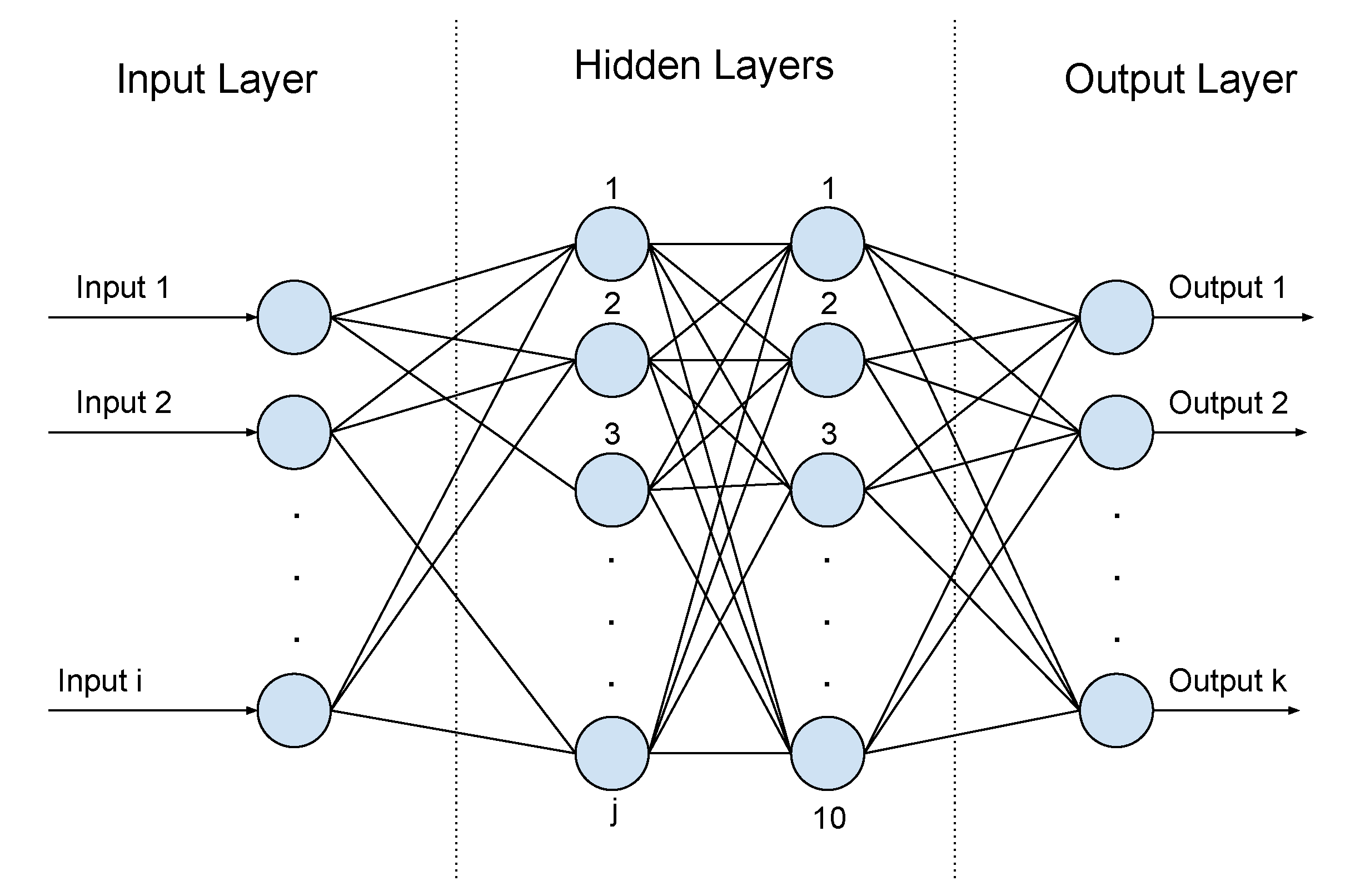
Figure 2.
The raw data of six different classes plotted on diagrams. The left and right lines of the red squares correspond to the limits of the window, ranged 1000-20000
Figure 2.
The raw data of six different classes plotted on diagrams. The left and right lines of the red squares correspond to the limits of the window, ranged 1000-20000
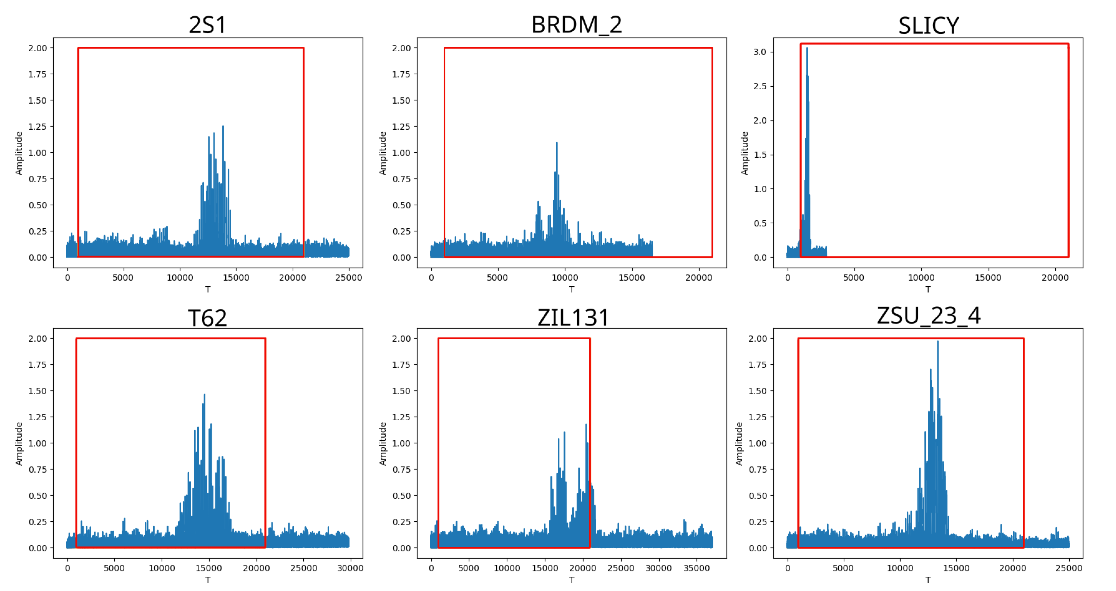

Table 1.
SOC results on differing networks.
| Layer 1 | Layer 2 | #Total Parameters | Estimated Total Size (MB) | Test Accuracy |
|---|---|---|---|---|
| 60 | 10 | 1,500,714 | 5.82 | 99.896% |
| 50 | 10 | 1,250,637 | 4.87 | 99.948% |
| 40 | 10 | 1,000,527 | 3.91 | 100.00% |
| 30 | 10 | 750,417 | 2.96 | 100.00% |
| 20 | 10 | 500,307 | 2.00 | 100.00% |
Table 2.
SOC results of different networks with the smaller window size.
| Layer 1 | Layer 2 | #Total Parameters | Estimated Total Size (MB) | Test Accuracy |
|---|---|---|---|---|
| 60 | 10 | 1,200,747 | 4.66 | 100.00% |
| 50 | 10 | 1,000,050 | 3.89 | 100.00% |
| 40 | 10 | 800,527 | 3.13 | 100.00% |
| 30 | 10 | 600,417 | 2.37 | 100.00% |
| 20 | 10 | 400,020 | 1,60 | 99.948% |
Table 3.
SOC results of different networks with the smaller window size and data sampling.
| Layer 1 | Layer 2 | N | #Total Parameters | Estimated Total Size (MB) | Test Accuracy |
|---|---|---|---|---|---|
| 60 | 10 | 2 | 600,747 | 2.33 | 100.00% |
| 4 | 300,747 | 1.17 | 100.00% | ||
| 8 | 150,747 | 0.59 | 99.849% | ||
| 50 | 10 | 2 | 500,637 | 1.95 | 99.948% |
| 4 | 250,637 | 0.98 | 99.844% | ||
| 8 | 125,637 | 0.49 | 99.896% | ||
| 40 | 10 | 2 | 400,527 | 1.57 | 100.00% |
| 4 | 200,527 | 0.78 | 100.00% | ||
| 8 | 100,527 | 0.39 | 99.896% | ||
| 30 | 10 | 2 | 300,417 | 1.18 | 99.948% |
| 4 | 150,417 | 0.59 | 99.844% | ||
| 8 | 75,417 | 0.30 | 99.896% | ||
| 20 | 10 | 2 | 200,307 | 0.80 | 99.896% |
| 4 | 100,307 | 0.40 | 99.896% | ||
| 8 | 50,307 | 0.20 | 99.896% |
Table 4.
EOC results on differing networks.
| Layer 1 | Layer 2 | Final Accuracy | Best Epoch | Best Accuracy |
|---|---|---|---|---|
| 60 | 10 | 80.36% | 6 | 81.06% |
| 50 | 10 | 98.96% | 4 | 99.22% |
| 40 | 10 | 99.04% | 2 | 99.48% |
| 30 | 10 | 97.91% | 6 | 98.70% |
Table 5.
EOC results of a network with the reduced input window size and data sampling.
| N | #Total Parameters | Estimated Total Size (MB) | Final Accuracy | Best Epoch | Best Accuracy |
|---|---|---|---|---|---|
| 1 | 800,494 | 3.13 | 96.09% | 6 | 99.39% |
| 2 | 400,494 | 1.57 | 98.96% | 8 | 99.48% |
| 4 | 200,494 | 0.78 | 98.87% | 6 | 99.48% |
| 8 | 100,494 | 0.39 | 97.22% | 5 | 98.18% |
Table 6.
Accuracies of neural networks used in related works and of the proposed networks.
| Dataset | Network | Conditions | Accuracy | |
|---|---|---|---|---|
| IMG | MSTAR [4] | A-ConvNet [10] | SOC | 99.13% |
| EOC | 87.40% | |||
| contrast-balanced | 98.00% | |||
| ResNet18 [18] | contrast-balanced | 98.90% | ||
| AP-CNN [12] | SOC | 98.10% | ||
| EOC | 93.57% | |||
| CNN-LSTM [14] | SOC | 99.38% | ||
| EOC | 95.57% | |||
| Yoon et al. [21] | SOC | 99.79% | ||
| EOC | 98.52% | |||
| OpenSARShip [16] | – | 84.25% | ||
| HOG-ShipCLSNet [15] | – | 78.15% | ||
| FUSAR-Ship [17] | – | 86.69% | ||
| IMG GBSAR [26] | ResNet18 [22] | – | 97.85% | |
| RAW | RCShip [27] | FastRCDet [24] | – | 77.12% |
| RAW GBSAR [28] | ResNet18 [23] | – | 93.06% | |
| MSTAR [4] | Proposed Networks | SOC | 99.90% | |
| EOC | 98.87% |
Table 7.
Power consumption and inference time of the proposed network on the tested embedded devices
Table 7.
Power consumption and inference time of the proposed network on the tested embedded devices
| Device | Power Consumption (W) |
SOC Inference Time (ms) | EOC Inference Time (ms) |
|---|---|---|---|
| NVIDIA RTX 4080, CUDA 12.0 | 320 | 0.23 | 0.29 |
| Khadas VIM3 | 4.084 | 21.60 | 21.75 |
| Raspberry Pi 5 | 5.458 | 1.53 | 1.83 |
Disclaimer/Publisher’s Note: The statements, opinions and data contained in all publications are solely those of the individual author(s) and contributor(s) and not of MDPI and/or the editor(s). MDPI and/or the editor(s) disclaim responsibility for any injury to people or property resulting from any ideas, methods, instructions or products referred to in the content. |
© 2025 by the authors. Licensee MDPI, Basel, Switzerland. This article is an open access article distributed under the terms and conditions of the Creative Commons Attribution (CC BY) license (http://creativecommons.org/licenses/by/4.0/).
Copyright: This open access article is published under a Creative Commons CC BY 4.0 license, which permit the free download, distribution, and reuse, provided that the author and preprint are cited in any reuse.


