Preprint
Article

This version is not peer-reviewed.

An Experimental Study Of The Vortical Structures In Supersonic Steam Jet Impinged On To The Wall

Submitted:

17 January 2025

Posted:

20 January 2025

You are already at the latest version

Abstract

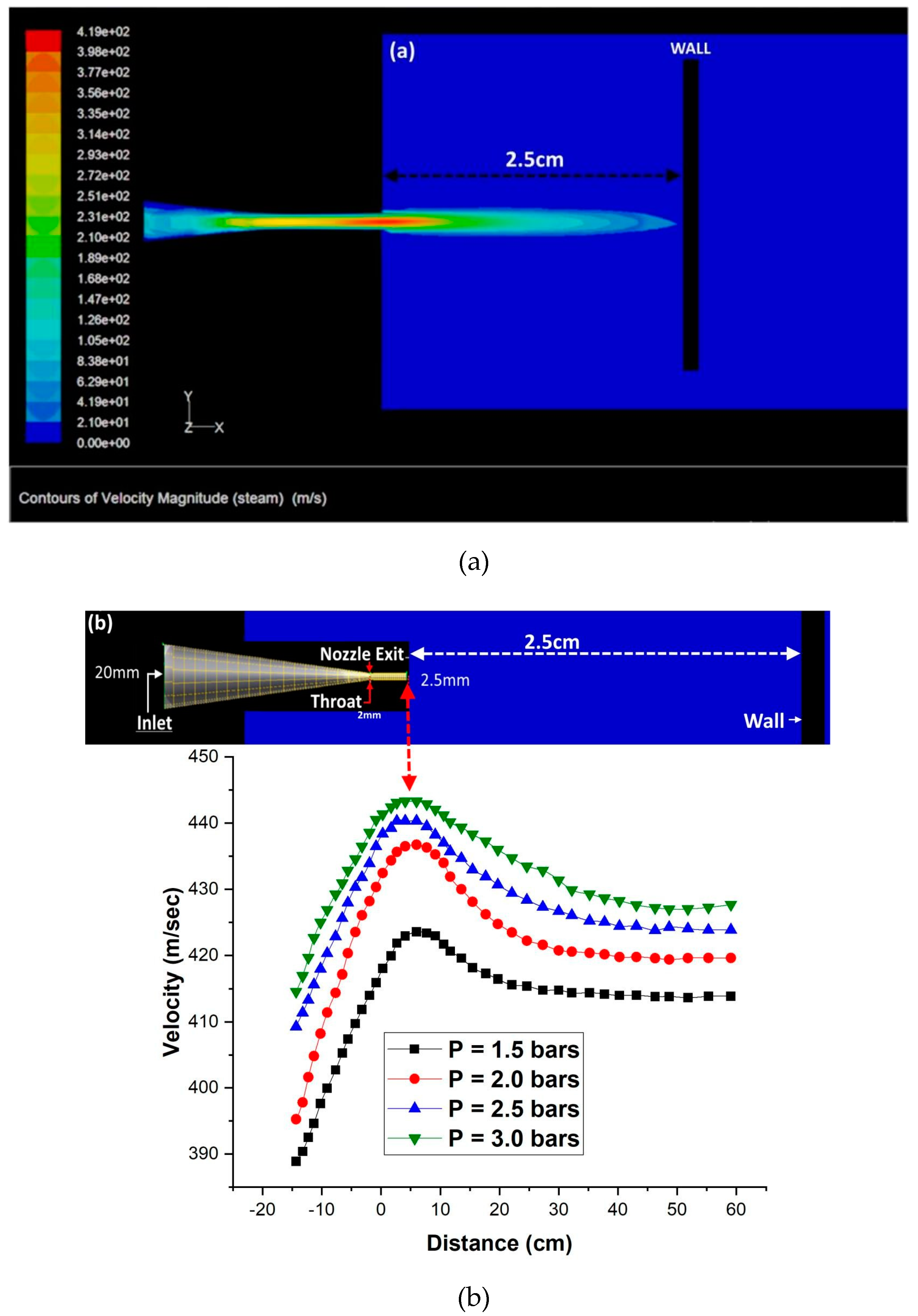
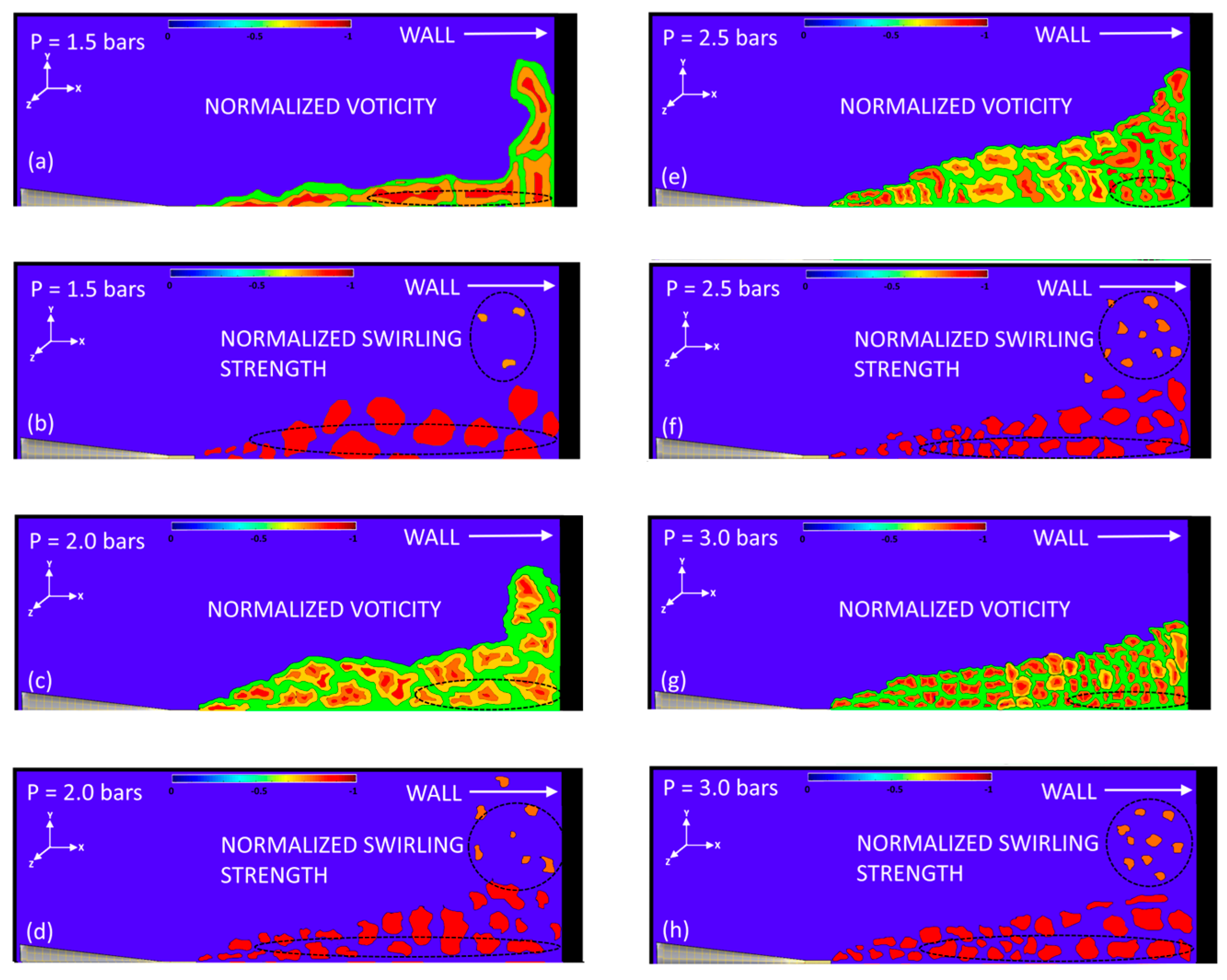
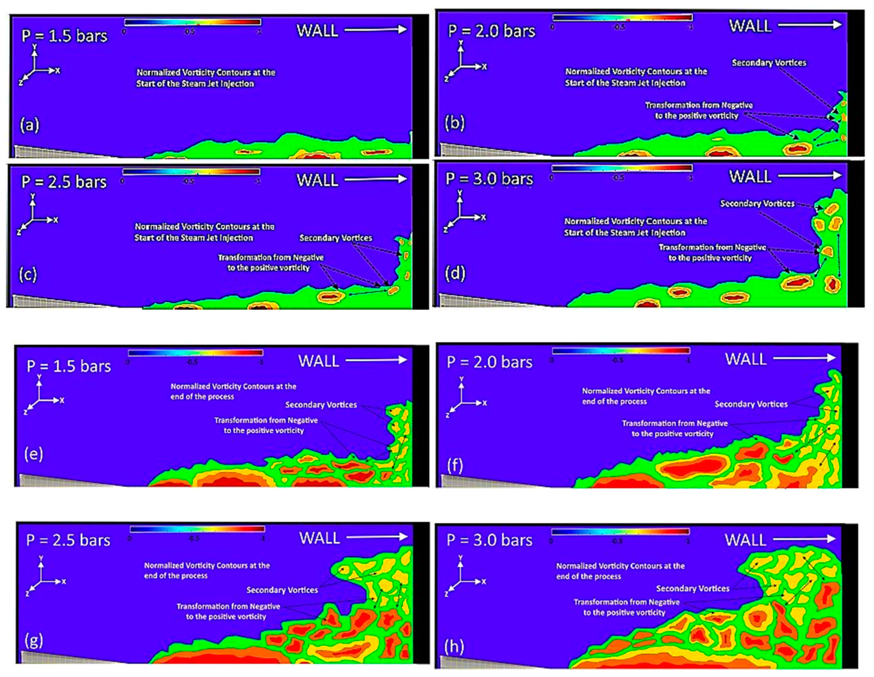
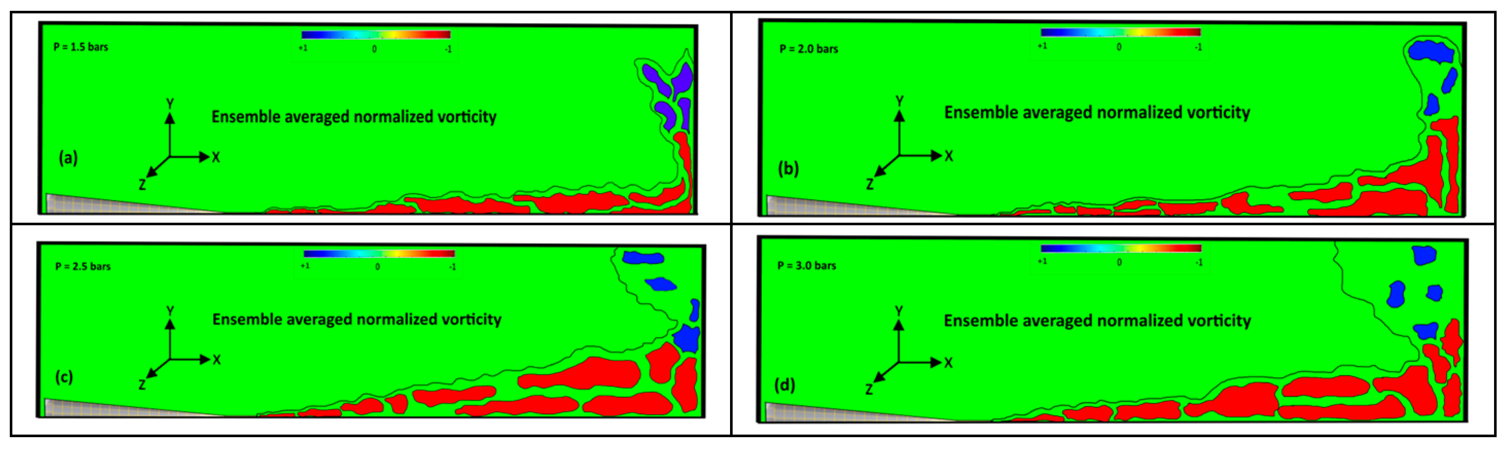
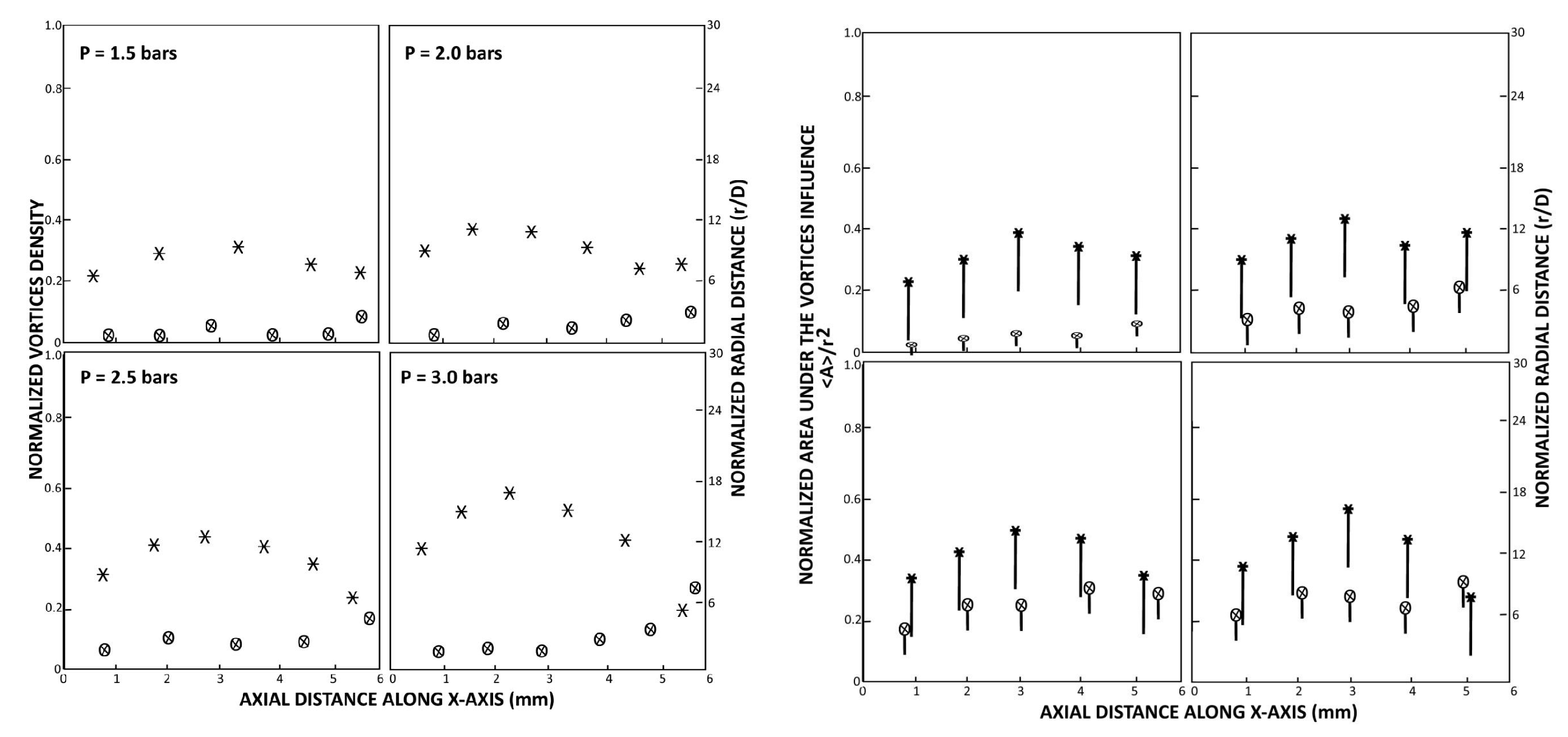
This study presents an experimental investigation into the impingement of a supersonic steam jet onto a wall. Steam was injected through a supersonic nozzle at a varying total pressure of 1.5-3.0 bars, producing a supersonic steam jet at a pressure gradient of 0.5-2.0 bars. The whole fluid domain is comprised of two regions: the jet region and the region near the wall involving the impingement of the supersonic steam jet. Within this region, the transformation of primary vortices into secondary vortices occurs and these vortices expel outward in the radial direction after impingement. Measurements have shown the spreading of the normalized density of the vortical structures along the axial length within the region near the wall. However, the probability density function analysis has indicated that the vortical structures become denser within the impingement region. Whereas subsequent to an impingement of the steam jet onto the wall, along the radial direction, weak traces of their existence in the jet region may be attributed to the vorticity diffusion within the jet region.

Keywords: 
;  ;  ;  ;  ;  

1. Introduction

When a jet, either consisting of the same fluid in its surroundings or a different one, impinges onto a wall and spreads in the surroundings along the radial direction to the jet, the characteristics of such a fluid domain are a combination of the hydrodynamics of the free jet as well as of the fluid within the boundary wall [1]. The jet will face retardation due to the surrounding fluid and the boundary wall. Thus, structures comprising vortices within such fluid domains are generated, which resemble closely with the structures that appear at the boundary of the interacting fluids. Furthermore, it has been observed that structures within the vicinity of the central jet or across the jet stream have close resemblance with those appearing at the periphery and surroundings of such vortices. The former has been termed as the primary vortices and the latter as the secondary vortices. The fluid present within the jet repels from the central region, whereas, the surrounding fluid is entrained into the mainstream of the fluid jet. Besides their resemblance to each other, a slight variation in their shapes may be attributed to the variations in the boundary conditions associated with them [1]. A significant volume of research has been conducted by the scientific community in this regard, which included studies involving air traveling within water and smoke was used as tracer particles [2]. In the current manuscript, the impingement of supersonic steam jet onto a wall has been studied. Steam jet interactions with the structures have myriad applications that range from steam interaction with turbine blades, textile products manufacturing, steam usage in the metal processing industry and in the paper industry, and a lot more can be narrated in this regard. Yet all these application areas enlighten the steam interaction with some solid body/wall, however, for further attention on this topic till date, only few studies have narrated the hydrodynamics of the fluid domain, focusing their interaction with the wall [3,4,5,6]. The vortical structures are formed when a supersonic steam jet impinges onto a wall at 90o, and such study requires detailed attention from the scientific community and the present manuscript is an effort in this regard. Jet impingement onto a wall was discussed in many studies, where the jet was generated using a converging nozzle. In such studies, the jet flow domain was characterized by the potential core region, which was stretched over 4-5 D (where D is the diameter of the nozzle exit) [7,8,9]. Other significant parameters being involved in such supersonic steam profile, include Reynolds number, distance between the nozzle and the wall, the jet exit velocity profile, the turbulence level [10], and the jet configuration and the shape of the nozzle [11]. The supersonic steam jet emerges from a converging- diverging nozzle. It is characterized by the nozzle design, as even at a very lower pressure gradient it is capable of producing the supersonic velocity profiles at its exit, as mentioned in our previous studies [12,13,14,15,16]. Following along the axial and radial directions (axial length L = 0 → L = ∞) & (r = 0 → r = r) respectively, the transformation of initially supersonic steam jet takes place from a uniform nature flow along the central axial line, with a thin shear layer near the nozzle exit, to a fully developed flow at far off locations. This includes scenarios like a radially expanding turbulent jet after impingement with the wall. Due to the inherent different nature of the fluid domains which are inhibited by the region that comprises of the jet around the nozzle exit [17], the region of the jet impingement [18], and the region where the jet expands [8], it is very difficult to simulate the whole of the fluid domain using a single turbulence mechanism [19]. The occurrence of the vortices and the interaction between them have a strong influence on the heat, momentum and mass transfer across the fluid domain and their interaction has been analyzed using equation 1 (Vorticity equation).
D ω D t = ω t + u . ω = ω . u ω . u + 1 ρ 2 ρ × ρ + × . Τ ρ + × B ρ
Where ω is the vorticity, t is time (s), u is the axial velocity (m/s), ρ is the fluid density (kg/m3), T is the viscous stress tensor and B is the sum of the external body forces. By using the experimental setup described in the latter section, the vortical distributions, the area under their influence as well as their swirling strengths are estimated. The details of the experimental setup and the outcomes extracted from the data are described in detail in the following sections.

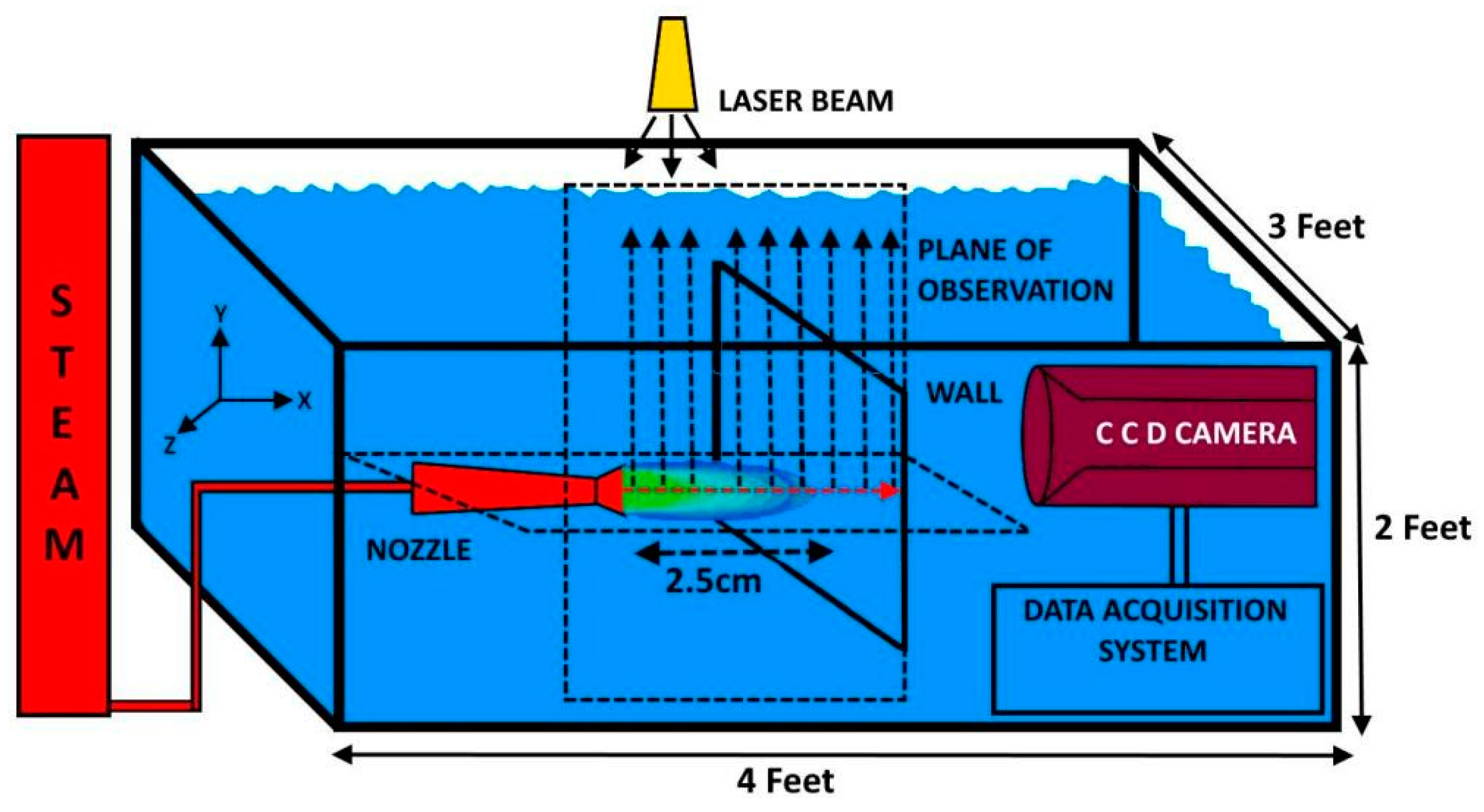
2. Experimental Setup

The experimental setup is comprised of a nozzle and a rectangular Perspex box. The nozzle geometry is shown in Figure 1. The capability of the nozzle with these dimensions has been confirmed to generate the supersonic jet flow in our previous studies [12,13,14,15,20]. The CFD study involves application of steady state model in the Ansys Fluent. The steam has been simulated by using the Direct Contact Condensation (DCC) Model [21]. The physical flow details of the DCC model including the key equations and the operating parameters are followed. In Direct Contact Condensation (DCC) model, each phase has been regarded as interpenetrating continua.
Each phase has its own governing equations representing the energy, momentum and continuity, and the coupling between these equations has been achieved by using the interphase exchange and pressure coefficients. Realizable model has been used to compute the turbulence and the symmetric model has been used for the drag formulation between the phases.
The continuity equation for the phase is given by,
t α q ρ q + . α q ρ q v q = p = 1 n m ˙ p q m ˙ q p + S q
whereas, is the velocity of the tℎ phase, is the rate of mass transfer from tℎ to tℎ phase, is the rate of mass transfer from tℎ to tℎ phase and is the source term. The governing equation for the momentum transfer is given by,
t α q ρ q v q + . α q ρ q v q v q = α q P + . τ q + α q ρ q g + p = 1 n R p q + m ˙ p q v p q m ˙ q p v q p + F q + F l i f t , q + F v m . q
Whereas v p q & v q p are the interphase velocities, F q is the external body force, τ q is the q t h phase stress strain tensor with F v m . q is the virtual mass force, & F l i f t , q is the lift force R p q is the interaction force between the phases and P is the pressure shared by the phases. The governing equation for the energy is given as;
t α q ρ q h q + . α q ρ q u q h q = α q P q t + τ q :   u q q q + S q + p = 1 n Q p q + m ˙ p q h p q m ˙ q p h q p  
Whereas, h q , q q ,   S q , are the specific enthalpy, heat flux, and the source term of the q t h phase, and Q p q ,   &   h q p   are the intensity of the heat exchange and enthalpy between the p t h and q t h phases. The details of the simulation conditions and the models used are given in the Table-01.
Table 1. Boundary conditions and details of the models used.
Phase Density Dynami c Kinem atic Youn g’s Poisso n’s press ure Tempera ture (0C) Ultim ate
(kg/m Viscosit Viscosi modu ratio (bars Tensil
3) y ty lus ) e
((Pa s, Ns/m2) x ((m2/s)x 10-6) (GPa) Strength
10-3) (MPa)
Const
ant value take Water from 0.798- 0.801- --- ---- Outlet press ure=1 bar 250C ----
Steam Co nstant value taken from Fluent data base Fluent data base Fluent data base --- --- Nozzl e Inlet= 1-3bars 100-1340C [22] ---
Model Solver: Pressure based
Formulation: Implicit
Multiph ase model Scheme: Euler 2 Phase
Viscous Model: k-epsilon 2 equations
k-epsilon: Realizable
Near wall treatment: Standard wall function
k-epsilon multiphase model: Mixture
Drag Steam-water: Symmetric
Heat: Ranz-Marshall
Mass transfer: Will be determined by User Defined Function (DCC model)
Under relaxation factor: 0.1
Pressure-velocity coupling: Phase coupled SIMPLE
Discretization: First order upwind
Multigrid control Cycle type: F- Cycle
Termination restriction: 0.1
AGM method stabilization method: Aggregative- BCGSTAB
Convergence criteria: 1 e-5
Direction of pressure specification method: Normal to the boundary Turbulence specification method: k-epsilo
Steam is injected through the inlet at a total pressure of 1.5-3.0 bars, which then flows through the nozzle. The nozzle is capable to induce supersonic flow at the given pressure range. The Perspex box has dimensions Length, L = 4 feet, Height, H = 2 feet, and Width, W = 3 feet (a schematic of the setup is shown in Figure 2). The nozzle is inserted into the box through a pipe insulated with heavy Teflon taping to preserve the quality of the injected steam. The distance between the nozzle and the wall is 2.5 cm. Velocity measurements have been obtained by using a particle image velocimetry (PIV) system, however, due to the physical limitations, just half of the whole region could be scanned using the PIV technique. This has been caused by the body of the nozzle hindering the laser light in the downward region of the nozzle. The PIV system consists of a charged coupled diode camera with resolution 2048 x 2048 ~ 7.4 μm2 pixels.
The laser has a pulse frequency of ~15 Hz and power 200 mJ/pulse with a National Electronics data acquisition and data processing software module. Fluorescent 1.0 g/cc microspheres have been used as tracer particles in this setup. The laser sheet was directed on the downward vertical configuration from the top whereas the position of the camera was aligned horizontally with the nozzle to take the PIV snaps at the mentioned frequency. Data has been acquired for 10 minutes and at a rate of 10 Hz. Thus, using this configuration, 6000 frames were acquired in 10 minutes against a single operating condition.
The frame for the CCD camera has been adjusted in such a way that it only focuses on the area shown by the upward dotted arrows in Figure 2. Anomaly detection has been performed into the generated frames to remove the uneven data points from the PIV frames. The calibration of the PIV system has been done through the use of a method that incorporates the accurate measurement of the laser pulse magnification and separation. The pulse separation has been measured by focusing the laser sheet on the photodetector, which itself has been connected to the oscilloscope. This indicates towards existence of estimated separation with respect to the distance between the point of light emergence and the point of light incidence on the photodetector. The magnification related errors have been measured by focusing the laser sheet light on a known dimension grid, being followed by taking the ratio of the measured grid spacing with the known grid spacing. This helps to estimate the extent of the optical distortions. If there is no distortion, then ratio value remains the same at all the locations along the fluid domain. The measurement uncertainties in the current case are around 0.1-0.3%. The distribution of vortical structures and the area under the influence of the vortices and their swirling strengths have been estimated using the relations which are described in detail in the proceeding section.

2.1. Mathematical Formulations

For the last two decades, the amount of information gathered using experimental and theoretical methods for the understanding of turbulence has grown appreciably. These include the common methods (e.g., hot wire method) used for the study of turbulence. Whereas on experimental grounds the PIV, and holography and on theoretical grounds Direct Numerical Simulation (DNS) and Large Eddy Simulation (LES) are the preferred methods. These methods discern well the dynamics, kinematics and scale resolution to extract the information related to the fluid domain. Reynold’s stress decomposition into its constituents i.e., the mean and fluctuating parts provide enough insight into the flow domain.
Yet these methods may prove successful to deliver correct components of Reynold’s stress, however, they have been proved not ideal to provide a clear understanding of the inhibiting flow process. The best method for drawing the complete picture of the process depends on the nature of the inhibited process and the goal to be achieved. In terms of statistical inter-relationship, Reynold’s decomposition method may prove to be the best choice. In view of the understanding of the structures and elements of the flow, the visualization methods can provide a deeper insight into the flow structures. However, the interaction between the smaller eddies and their interaction with the large flow structures can be exhibited through the detection of the smaller eddies. Also, the visualization of the streak lines across a fluid domain has been conducted. Even having our weak confidence on such techniques to offer accurate flow picture, however, such information has been obtained here to exhibit characterization of physical quantities. As illustrated by the studies [23,24], the streak lines roll up in a false manner in a flow that shows the presence of discrete vortices. Alternatively, the choice of the reference frame has immense importance as steady flows can appear unsteady in an incorrect frame of reference. The identification of the vortices in a vector field along with their diameter and strength calculations is normally accomplished by identifying regions of isolated nature, i.e., the regions containing higher strength of vorticities. In simple flow fields this may be an easy task, but in complex flow regimes this is not an easy task. In such a case, the vortices within a flow regime may be masked by the shearing flow profiles, thus making it difficult to identify the vortices and then to identify their contribution to the overall flow. The method to identify the state of motion of a fluid regime depends on the critical point estimation of the local velocity gradient tensor and its corresponding eigenvalues [25,26,27,28]. In a 3D domain, the velocity gradient tensor will have one real eigenvalue (λr) and a pair of complex conjugate eigenvalues (λcr±iλci). Now, here two conditions can be raised, first when the discriminant of the
equation is positive then the particles exhibit a swirling motion and 1 represents the period required to revolve around the axis of the . On the other hand, when is equal to zero, then the path of the particles is infinitely elliptical, and the flow would be the shearing flow. Thus, the vortex study using data of the swirling strength is independent of the frame of reference as it does not give any information related to the regions having the maximum vorticity, but these represent the regions that lack any swirling motion.
The relations used for the calculations of the vorticity and swirling strength is given by ψ θ = U x r U r x , and Ω c i = λ c i φ θ φ θ , which offers insight of the vortical structures [29]. It should be noted that among all the methods being applied for vortex extraction, the method of determining the swirling strength has proved very useful, especially when dealing with wall turbulence [30,31,32,33,34,35,36]. The method for the swirling strength determination was determined by Zhou. et. al. [28]. However, the method was developed further [37,38], and the swirling strength as an imaginary part of the complex eigenvalues for the velocity gradient tensor, was defined [39], which offeredan excellent vortex indicator in wall turbulence involving strong mean shear. Since the vorticity is the square of the angular velocity, it has been normalized by dividing it with the square of the maximum axial velocity U m 2 .   i.e., ω 2 U m 2 .
Also, the Probability Density Function (PDF) analysis has been performed by estimating the likelihood of the occurrence of the primary and secondary vortices across a PIV plane using the MATLAB Blob analysis tool [40]. Probability Density Function (PDF) analysis has been performed to the whole of the fluid domain to identify the regions of maximum primary and secondary vortices, which rely on the nature of their clockwise and anti-clockwise rotations. The central point of such regions is located and the area under the influence of such vortices along with the strength of these vortices [41] and their relative abundance have been calculated. The details regarding this Blob analysis tool has been given as follows.
Blob analysis is a machine-based technique which is based on the analysis of the consistent image regions. The objects have been analyzed, thus, tailored solutions for a wide range of visual inspection problems have been devised using this technique. In this technique first, all the images have been classified based on the color of the background, which is blue in our case and any other color shows the relative strength of the vortices. Thus, a combined histogram has been build based on the equation given below [42],
C j = m a x w m M j w B B j C m a x , 0 × D
Whereas, j represents the index of each histogram bin, the combined histogram maximum value has been shown here by C m a x , with the output range D. The colors of each pixel has been assigned value based on the classification, through which original RGB have been converted into normalized color spaces;
r = R R + G + B , g = G R + G + B , & b = B R + G + B
The central position x c , y c   and the velocity v i   of each blob has been estimated as;
x c = M 10 M 00 ,   y c = M 01 M 00  
v i   = ( x c i x c i 1 ) 2 + ( y c i y c i 1 ) 2   T  
Whereas;
M 00 = x y I x , y ,     M 10 = x y x I x , y ,   M 01 = x y y I x , y ,  
With M 00 ,   M 10 ,   &   M 01 are the first order moment calculated from the image intensity I x , y .   The second order moments of the area have been calculated as;
  M 20 = x y x 2 I x , y ,   M 02 = x y y 2 I x , y ,  
Which helps us calculate the major and minor axis of the blobs as;
a = 6 p + r + q 2 + p r 2   ,
b = 6 p + r q 2 + p r 2    
Whereas;
p = M 20 M 00 x c 2 ,   q = 2 M 20 M 00 x c y c ,   r = M 02 M 00 y c 2  
Thus using these relations, the aspect ratio, size, and area of each blob has been calculated which onwards helps us to observe the relative abundance of the vortical shapes inside the fluid region. The results and the related discussion on the outcomes are given in the following section.

3. Results & Discussion

In the current study, the supersonic steam jet has impinged on a static wall, the resulting flow profiles, the vortices generation and their interaction, along with the area under their influence and their swirling strengths have been obtained with the help of the data acquired by using a PIV system. The results and outcomes at varying operating conditions have been presented and discussed in detail as follows.

3.1. Analysis of the Vortices

Our understanding regarding the submerged jet injection and the resultant vortices has evolved hugely during the last few decades. In the cited literature [43], the inter- connection between turbulence and the resulting vortices and their induced entrainment of the surrounding fluid has been discussed. A layer that superimposes over the turbulent layer, thus giving birth to a surface that is immersed between these two layers, i.e., the turbulent layer and the overlapping layer of the non-turbulent fluid around it. These layers have relatively at simple configuration with each other and marked with instantaneous boundary layer based on the structures of the interacting fluids inside them. Thus, the vortices that have been created due to the shear of the turbulent high velocity fluid layer can appropriately be described as the diffusive propagation of the turbulent layer into surrounding fluid layer across the interface between them. In such scenarios, the random diffusive propagation of the turbulent layer into the surrounding fluid layer resulting into the nibbling of the surrounding fluids, whereas the non-turbulent surrounding fluid layers have been characterized by the main core region flow boundary [44,45]. Yet the whole process has resulted into the creation of the vortices across the interface, as well as the entrainment of the surrounding fluid, this whole sequence should be divided into three phases. In the first part, the middle layer and the non-turbulent layer have been set into motion by the main core turbulent flow. The initiation of the motion of the middle and top fluid layers will be governed by the turbulent boundary that will act to bring the top two layers intermittent to each other with subsequent formation of vortices characteristic of the top two layers. In the second phase, the main core turbulent flow will come into a connection with the motion of the top two-layer, as these two layers will start reducing their thickness till Kolmogorov scale, which has been termed as nibbling as previously mentioned. At this scale, the top two layers have mixed with the turbulent fluid under the action of viscosity and diffusion processes. This stage can be termed as “Turing” through the rapid decrease in the thickness of the intimate surrounding fluid layers. The last stage is marked with clear mixing, where the possibility of coalescence of the elements of the turbulent fluid, which may affect mixing and entrainment process.
When the supersonic steam jet has impinged on a wall, the jet flow domain must counter multiple retarding mechanisms (that include the jet quenching by the wall as well as the retardation being offered to the jet by the surrounding fluids. Normalized vorticity and its swirling strength have been determined and plotted at different inlet pressures (1.5-3.0 bars) as shown in Figure 3a–h.
It should be noted that these plots have shown the intermediate stages of the flow in between the events when the steam has been injected and the event when the supply of the steam has been terminated at the start and the end of the data acquisition phase respectively.
It has been observed that at the central region of the plane, the normalized negative vortices have maxima whereas this behavior degrades as soon as the jet moves outward along the radial direction, after the jet striking the wall. This has been shown by the circular marks in Figure 3a–h. A possible reason for such a behavior may be that the fluid at high velocity induced vortical structures at its interface with the surrounding water. These vortical structures have positive vorticity with respect to the negatively vorticity fluid elements at its interface. These negative vortical structure fluid elements have more concentration at the center which gradually reduce as the vortical structure fluid elements move away from the central portion.
The vortical structures and their swirling strengths have been determined using the relations given before. The vortical structures are present both in the jet region as well as near the wall region. However, at lower inlet pressure, a clear indication occurs towards the existence of the Kelvin Helmholtz instabilities, which act within the fluid layers resulting in the vorticities that rotate in anti-clockwise directions. These are the vortical structures encapsulating the round jet, which results in sustained enveloping profiles around the jet which afterwards break near the wall into small vortical structures and being expelled radially outwards. The distance, by which the enveloping vortical structures encapsulating the main round body of the jet, ranges from 0 D to 3.0 D. This is the standoff distance at which the nozzle is placed away from the wall.
The enveloping vortical structures encapsulate the round body of the jet before they strike with the wall, resulting in the structures quickly spreading out due to the radially expanding shear layer near the wall, this then tears them into small vortical structures moving away from the striking/impingement point. These are the secondary vortices (shown by the orange color contours in each figure). Large secondary vortices don’t appear across the region when the jet reaches to impinge at the wall. These large vortices are not clearly detected in the region even near the wall, rather a densely populated region (secondary vortices) near the wall will give rise to the vortices of different sizes and shapes across this chaotic region.

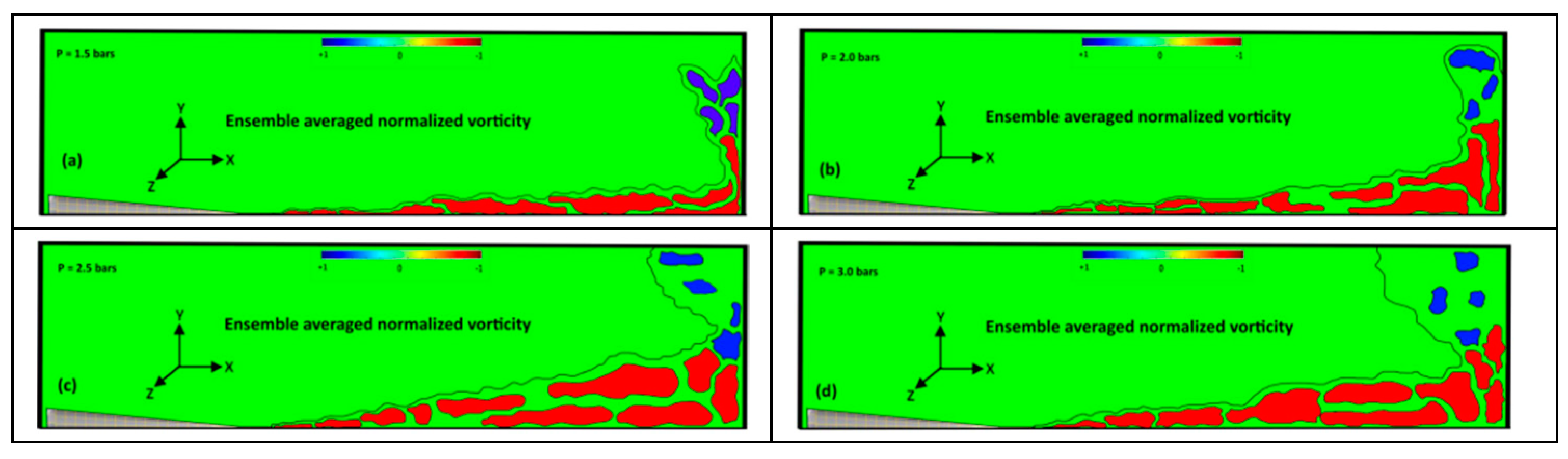
3.2. Transformation from Negative to Positive Vortices & Their Spatial Occurrence Probability

The formation of the vortical structures inside the two-phase flows and their transformation from negative to the positive vortices or vice-versa has a lot of implications in the fluid dynamic studies of multiphase flows. Starting from the propagation of the shockwaves in two-phase flows [46] to fast growing droplets in clouds, where the clustering of such vortices resulted into an increased concentration of the water contents after collisions among cloud’s entities [11,12] etc. The vorticities and their swirling strengths indicate the most traveled tracks and the shearing layers as shown in Figure 4a–c.
The clockwise vortical structures have been transformed into a thick layer of fluid vorticities which will be generated due to the turbulence induced by the impingement of the primary vortical structures on to the wall. The transformation of the primary vortices into the secondary vortices occurs in the region along the radial axis from a distance of r = 10 mm till r = 30 mm with pressure varying from 1.5 to 3.0 bars (Figure 5a–d). It should be noted that in Figure 5a–d the normalized vorticity has been shown at the start of the process. Whereas, just few seconds before the end of the process the normalized vorticity contours have been shown in Figure 5e–h.
It has been observed from the contours of the normalized vorticity, that the density of the transformed positive vortices is very low at the start of the process. At the end of the process, the density of these positive vortices is considerable as shown in Figure 5e–h).
These vortices exist in the region near the nozzle exit and, in the region, where enveloping vortices are generated all the way to the region near the wall. These positions along with the axial axis range from X/D = 0 till ~3 corresponding to the inlet pressure, P = 1.5-3.0 bars.
Along the normalized radial distance (r/D), the profiles for the ensembled averaged swirling strengths were estimated from r/D = 0 to r/D = 15. In this regard, to clarify the existence of the primary and secondary vortices, and their spatial transformation from primary to secondary vortices, Probability Density Function (PDF) analysis has been performed to the whole of the fluid domain to identify the regions of maximum primary and secondary vortices, relying on the nature of their clockwise and anti- clockwise rotations. The central point of such regions is located and the area under the influence of such vortices along with the strength of these vortices [41] and their relative abundance have been computed as shown in Figure 7a,b.
From Figure 7a,b, with an increase in the inlet steam pressure, there is a slight increase in the number of primary vortices in the surroundings of the main jet region. However, in the near-wall region, a small increase in the density of the dimensionless secondary vortices is observed. These results have been supported by an increasing trend in the area under the influence of the primary and secondary vortical structures. The normalized vortical structures density for the primary vortices have shown an increasing trend in terms of their number density that ranges from 0.2 to 0.6 for primary vortices, and from 0 to 0.3 for secondary vortices. Whereas in terms of the normalized area ratio ,, the range stretches between 0.02 and 0.6 for primary vortices and 0.01 and 0.3 for secondary vortices within the surroundings of the jet and in the near-wall region respectively. The impingement region and the near-wall region following the impingement are characterized by the length (X = 5-6mm), which corresponds to the stand-off distance between the supersonic steam jet nozzle and the normalized radial distance (r/D) that ranges from 0-30. Whereas, the normalized primary vortical structure density peaks exist at 0.27 and the secondary vortical structures density peaks exist at 0.22. Also, the normalized area under the influence of the primary vortical structures peaks exist at 0.4 and the area under the influence of the secondary vortices structures peaks exist at 0.3 in these regions. Furthermore, in these regions, in most of the cases, the normalized vortical structure density and the area under the influence of these vortical structures are found to be decreasing. However, this slight decrease may be attributed to the vorticity diffusion [47].

Conclusions

In the current manuscript, an experimental study has been undertaken, involving impingement of a supersonic steam jet onto a wall. The characterization of jet’s impingement is based on the generation of primary and secondary vortices as well as their normalized swirling strengths. It has been found that with an increase in the total inlet pressure from 1.5-3.0 bars, the normalized vortical structures density distribution has spread widely, which gives birth to the region of extremely chaotic activities. Primary vortices have been transformed into secondary vortices within the impingement region and in the near-wall region, where they are found to be expelled outward along the radial direction after the impingement. The density distribution of the normalized vortical structure through the spatial Probability Density Function (PDF) analysis reveals that the maximum number of secondary vortices are born near the impingement region and the region after the jet impingement with the wall, along the radial directions, whereas, the probability of such vortices being detected within the jet region is small, which may be attributed to the diffusion of vortices into each other.

Acknowledgment

The authors are thankful to the Ministry of Science and Higher Education of the Russian Federation.

Nomenclature

Symbol Description
L Axial length (m)
r Radial length (m)
D Nozzle diameter (m)
t Time (s)
u Axial velocity (m/s)
B Sum of external forces
Greek symbols
ω Vorticity
ρ Fluid density (kg/m3)
Viscous stress tensor
Optimal in-homogeneous proper orthogonal decomposition (POD) basis function for the axial component of the velocity
Ω Swirling strength
Subscripts
x Along axial axis
r Along radial axis
θ Ensemble averaged

References

  1. P. Bakke, An experimental investigation of a wall jet, J. Fluid Mech. 2 (1957) 467– 472. [CrossRef]
  2. T. Deng, S. Norris, R.N. Sharma, Numerical investigation on the stability of tunnel smoke stratification under the effect of water spray and longitudinal ventilation, Tunn. Undergr. Sp. Technol. 112 (2021) 103901. [CrossRef]
  3. J. Lede, J. Villermaux, R. Ouzane, M.A. Hossain, R. Ouahes, Production of hydrogen by simple impingement of a turbulent jet of steam upon a high temperature zirconia surface, Int. J. Hydrogen Energy 12 (1987) 3–11. [CrossRef]
  4. X. Li, J.L. Gaddis, T. Wang, Modeling of heat transfer in a mist/steam impinging jet, J. Heat Transfer 123 (2001) 1086–1092. [CrossRef]
  5. C.B. Domnick, F.K. Bera, D. Brillert, C. Musch, Modification of a steam valve diffuser for enhanced full load and part load operation using numerical methods, Period. Polytech. Mech. Eng. 60 (2016) 185–192. [CrossRef]
  6. J. Woisetschläger, H. Jericha, W. Sanz, F. Gollner, Optical investigation of transonic wall-jet film cooling, ASME Cogen Turbo Power 95 (1995).
  7. M. Shademan, R. Balachandar, V. Roussinova, R. Barron, Round impinging jets with relatively large stand-off distance, Phys. Fluids 28 (2016). [CrossRef]
  8. B.E. Launder, W. Rodi, The turbulent wall jet, Prog. Aerosp. Sci. 19 (1979) 81–128. [CrossRef]
  9. Y.M. Chung, K.H. Luo, Unsteady heat transfer analysis of an impinging jet, J. Heat Transfer 124 (2002) 1039–1048. [CrossRef]
  10. C.J. Hoogendoorn, The effect of turbulence on heat transfer at a stagnation point, Int. J. Heat Mass Transf. 20 (1977) 1333–1338. [CrossRef]
  11. J. Lee, S.J. Lee, The effect of nozzle configuration on stagnation region heat transfer enhancement of axisymmetric jet impingement, Int. J. Heat Mass Transf. 43 (2000) 3497–3509. [CrossRef]
  12. A. Khan, K. Sanaullah, M. Sobri Takriff, A. Hussain, A. Shah, I. Rafiq Chughtai, Void fraction of supersonic steam jet in subcooled water, Flow Meas. Instrum. 47 (2016) 35–44. [CrossRef]
  13. A. Khan, K. Sanaullah, M.S. Takriff, H. Zen, A.R.H. Rigit, A. Shah, I.R. Chughtai, Numerical and experimental investigations on the physical characteristics of supersonic steam jet induced hydrodynamic instabilities, Asia-Pacific J. Chem. Eng. 11 (2016) 271–283. [CrossRef]
  14. A. Khan, CFD Based Hydrodynamic Parametric Study of Inclined Injected Supersonic Steam into Subcooled Water, in: 2014. [CrossRef]
  15. A. Khan, K. Sanaullah, M.S. Takriff, H. Zen, L.S. Fong, Inclined Injection of Supersonic Steam into Subcooled Water: A CFD Analysis, Adv. Mater. Res. 845 (2014) 101–107. [CrossRef]
  16. A. Khan, K. Sanaullah, N.U. Haq, Development of a Sensor to Detect Condensation of Super-Sonic Steam, Adv. Mater. Res. 650 (2013) 482–487. [CrossRef]
  17. A.J. Yule, Large-scale structure in the mixing layer of a round jet, J. Fluid Mech. 89 (1978) 413–432. [CrossRef]
  18. K. Nishino, M. Samada, K. Kasuya, K. Torii, Turbulence statistics in the stagnation region of an axisymmetric impinging jet flow, Int. J. Heat Fluid Flow 17 (1996) 193– 201. [CrossRef]
  19. N. Zuckerman, N. Lior, Radial slot jet impingement flow and heat transfer on a cylindrical target, J. Thermophys. Heat Transf. 21 (2007) 548–561.
  20. A. Khan, K. Sanaullah, M.S. Takriff, H. Zen, A.R.H. Rigit, A. Shah, I.R. Chughtai, T. Jamil, Pressure stresses generated due to supersonic steam jet induced hydrodynamic instabilities, Chem. Eng. Sci. 146 (2016) 44–63. [CrossRef]
  21. A. Shah, I.R. Chughtai, M.H. Inayat, Numerical Simulation of Direct-contact Condensation from a Supersonic Steam Jet in Subcooled Water, Chinese J. Chem. Eng. 18 (2010) 577–587. [CrossRef]
  22. E.B. Entry, STEAM TABLES, A-to-Z Guid. to Thermodyn. Heat Mass Transf. Fluids Eng. (2011). [CrossRef]
  23. F.R. Hama, Streaklines in a perturbed shear flow, Phys. Fluids 5 (1962) 644–650. [CrossRef]
  24. I. Gursul, D. Lusseyran, D. Rockwell, On interpretation of flow visualization of unsteady shear flows, Exp. Fluids 9 (1990) 257–266. [CrossRef]
  25. M.S. Chong, A.E. Perry, B.J. Cantwell, A general classification of three-dimensional flow fields, Phys. Fluids A 2 (1990) 765–777. [CrossRef]
  26. DALLMANN, U. , On the Footprints of Three-Dimensional Separated Vortex Flows Around Blunt Bodies, AGARD CP 494 (1991).
  27. J. Zhou, R.J. Adrian, S. Balachandar, Autogeneration of near-wall vortical structures in channel flow, Phys. Fluids 8 (1996) 288–290. [CrossRef]
  28. J. Zhou, R.J. Adrian, S. Balachandar, T.M. Kendall, Mechanisms for generating coherent packets of hairpin vortices in channel flow, J. Fluid Mech. 387 (1999) 353– 396. [CrossRef]
  29. R.J. Adrian, K.T. Christensen, Z.C. Liu, Analysis and interpretation of instantaneous turbulent velocity fields, Exp. Fluids 29 (2000) 275–290. [CrossRef]
  30. S. Herpin, M. Stanislas, J. Soria, The organization of near-wall turbulence: A comparison between boundary layer SPIV data and channel flow DNS data, J. Turbul. 11 (2010) 1–30. [CrossRef]
  31. S.J. Lee, Y.S. Choi, Decrement of spanwise vortices by a drag-reducing riblet surface, J. Turbul. 9 (2008) 1–15. [CrossRef]
  32. V.K. Natrajan, Y. Wu, K.T. Christensen, Spatial signatures of retrograde spanwise vortices in wall turbulence, J. Fluid Mech. 574 (2007) 155–167. [CrossRef]
  33. Y. Wu, K.T. Christensen, Population trends of spanwise vortices in wall turbulence, J. Fluid Mech. 568 (2006) 55–76. [CrossRef]
  34. W.T. Hambleton, N. Hutchins, I. Marusic, Simultaneous orthogonal-plane particle image velocimetry measurements in a turbulent boundary layer, J. Fluid Mech. 560 (2006) 53–64. [CrossRef]
  35. K.T. Christensen, Y. Wu, Visualization and characterization of small-scale spanwise vortices in turbulent channel flow, J. Vis. 8 (2005) 177–185. [CrossRef]
  36. K.T. Christensen, R.J. Adrian, Statistical evidence of hairpin vortex packets in wall turbulence, J. Fluid Mech. 431 (2001) 433–443. [CrossRef]
  37. C.D. Tomkins, R.J. Adrian, Spanwise structure and scale growth in turbulent boundary layers, J. Fluid Mech. 490 (2003) 37–74. [CrossRef]
  38. Q. Chen, R.J. Adrian, Q. Zhong, D. Li, X. Wang, Experimental study on the role of spanwise vorticity and vortex filaments in the outer region of open-channel flow, J. Hydraul. Res. 52 (2014) 476–489. [CrossRef]
  39. H. Chen, D. Li, R. Bai, X. Wang, Comparison of swirling strengths derived from two- and three-dimensional velocity fields in channel flow, AIP Adv. 8 (2018) 055302. [CrossRef]
  40. MATLAB, Statistics for labeled regions - Simulink, (n.d.).
  41. R.L. (Ronald L. Panton, Incompressible flow, n.d.
  42. S. Lu, G. Tsechpenakis, D.N. Metaxas, M.L. Jensen, J. Kruse, Blob analysis of the head and hands: A method for deception detection, in: Proc. Annu. Hawaii Int. Conf. Syst. Sci., 2005: p. 20. [CrossRef]
  43. S. Corrsin, A.L. Kistler, Free-Stream Boundaries of Turbulent Flows, Johns Hopkins Univ.; Balt. MD, United States (1955).
  44. J.L. Henk Tennekes, Hendrik Tennekes, John Leask Lumley, A First Course in Turbulence - Emeritus Professor of Aeronautical Engineering Henk Tennekes, Hendrik Tennekes, John Leask Lumley, J. L... Lumley - Google Books, MIT Press., 1972.
  45. F.H. Clauser, The structure of turbulent shear flow, Nature 179 (1957) 60. [CrossRef]
  46. N.N. Smirnov, N.I. Zverev, M. V. Tyurnikov, Two-phase flow behind a shock wave with phase transitions and chemical reactions, Exp. Therm. Fluid Sci. 13 (1996) 11– 20. [CrossRef]
  47. R. van Hout, V. Rinsky, Y.G. Grobman, Experimental study of a round jet impinging on a flat surface: Flow field and vortex characteristics in the wall jet, Int. J. Heat Fluid Flow 70 (2018) 41–58. [CrossRef]
Figure 1. (a) CFD Study based velocity contours [12,13,14,15,20] (b) Supersonic Nozzle Design with velocity profiles.
Preprints 146433 g001
Figure 2. A schematic of an experimental setup.
Preprints 146433 g002
Figure 3. (a-h). Normalized vorticity and Normalized Swirling Strength at the varying inlet total pressure 1.5-3.0 bars.
Preprints 146433 g003
Figure 4. (a-d). Ensemble average vorticity profiles at the varying inlet pressure (1.5-3.0 bars).
Preprints 146433 g004
Figure 5. (a-d). Transformation of negative to positive vorticity after impingement of ths steam jet with the wall (at the start of the process). (e-h). Transformation of negative to positive vorticity after impingement of the steam jet with the wall (at the start of the process). The profiles for the normalized swirling strengths can be seen in Figure 6a–d, which indicate the the strongest vortices reside within the fluid domain.
Preprints 146433 g005
Figure 6. (a-d). Ensemble average swirling strength at varying pressure ranges from 1.5-3.0 bars.
Preprints 146433 g006
Figure 7. (a). Normalized Vortices density ( × Primary vortices) & ( ⨂ Secondary vortices) across axial and dimensionless radial directions at varying pressure (1.5-3.0) bars. (b). Normalized Area under the vortical influence († Primary vortices) & (⨂ Secondary vortices) across axial and dimensionless radial directions at varying pressure (1.5-3.0) bar.
Preprints 146433 g007
Disclaimer/Publisher’s Note: The statements, opinions and data contained in all publications are solely those of the individual author(s) and contributor(s) and not of MDPI and/or the editor(s). MDPI and/or the editor(s) disclaim responsibility for any injury to people or property resulting from any ideas, methods, instructions or products referred to in the content.
Copyright: This open access article is published under a Creative Commons CC BY 4.0 license, which permit the free download, distribution, and reuse, provided that the author and preprint are cited in any reuse.
Prerpints.org logo

Preprints.org is a free preprint server supported by MDPI in Basel, Switzerland.

Subscribe

Disclaimer

Terms of Use

Privacy Policy

Privacy Settings

© 2025 MDPI (Basel, Switzerland) unless otherwise stated