
Submitted:
17 January 2025
Posted:
17 January 2025
You are already at the latest version
Abstract
This paper proposes a unified reliability analysis framework for mechanical and structural systems equipped with Tuned Mass Dampers (TMDs), encompassing single-degree-of-freedom (1-DOF), two-degree-of-freedom (2-DOF), and ten-degree-of-freedom (10-DOF) configurations. The methodology combines four main components: (i) probabilistic uncertainty modeling for mass, damping, and stiffness, (ii) Latin Hypercube Sampling (LHS) to efficiently explore parameter variations, (iii) Monte Carlo Simulation (MCS) for estimating failure probabilities under stochastic excitations, and (iv) machine lSome ML models, such as Random Forest (RF), Gradient Boosting (GB), Extreme Gradient Boosting (XGBoost), and Neural Networks (NN) are used to predict structural responses and failure probabilities. The results show that ensemble methods, such as RF and XGBoost, are accurate. They can highlight important features as well. Neural Networks work well for nonlinear behavior, however, careful tuning is necessary to prevent overfitting. We also extended to a 10-DOF structure. These simulation results show that ML-based models are useful for large-scale reliability analysis. These findings also show how simulation methods and data-driven models work together to improve the reliability of TMD systems under uncertain inputs.
Keywords:
Structural Reliability
; Tuned Mass Damper
; Machine Learning
; Multi-Degree-of-Freedom
; Surrogate Modeling
1. Introduction
Modern engineering structures ranging from tall buildings and long-span bridges to industrial machinery and aerospace components are becoming increasingly complex and are subjected to diverse and often stochastic loading conditions [1]. Ensuring that these systems maintain their structural integrity and reliability over their intended service life is of paramount importance. Traditionally, Structural Reliability Analysis (SRA) was employed deterministic or semi-probabilistic methods under simplified assumptions [2,3]. While these foundational approaches offer valuable insights, although these basic approaches provide valuable insights, they often cannot capture the true complexity systems because of the multiple sources of uncertainty such as material properties, geometric variations, environmental forces.
As industrial demands push for more sophisticated structures and integrate performance-based design principles, the need for more accurate and computationally efficient reliability assessment tools grows markedly [4,5]. Monte Carlo simulations, polynomial chaos expansions, and other uncertainty quantification methods have expanded the scope of SRA [6]; however, they frequently become prohibitively expensive when the number of uncertain parameters and the complexity of the structural model increase. This challenge is especially pronounced in multi-degree-of-freedom (MDOF) systems, where interactions among numerous components must be accurately accounted for. For example, many large-scale infrastructures and mechanical systems employ TMDs to mitigate vibrational responses [7,8,9]. Although TMDs can significantly reduce the likelihood of catastrophic failures under dynamic loading, their performance depends on a range of uncertain factors, including mass, damping, stiffness, and external excitation characteristics.
Tuned Mass Dampers [10,11,12,13] are widely used to reduce the harmful effects of dynamic forces from wind, earthquakes, and other external loads. Many studies focus on simple models like 1-DOF or 2-DOF systems to understand basic vibration control. However, real structures often have many degrees of freedom. This makes modeling and reliability analysis more complex and computationally demanding. In the presence of uncertainties in parameters and external loads, The MCS has established itself as a robust technique for assessing structural reliability, particularly for random vibration problems [14,15]. However, the high computational cost of exhaustive simulations can become impractical as the number of degrees of freedom and thus the complexity increases. Recent research [16,17,18,19,20] has explored hybrid strategies that combine simulation-based approaches with ML to address this computational burden [21,22]. In these approaches, ML models serve as surrogate predictors for system responses, thereby reducing the overall number of high-fidelity simulations required.
This article unifies these concepts within a single framework, examining TMD-enhanced reliability from low-DOF to multi-DOF structural systems. First, low-degree-of-freedom setups are introduced as foundational cases, illustrating how TMD-equipped systems can be effectively modeled and how machine learning surrogates are constructed. The study then expands to a 10-DOF building-like structure, which represents a more realistic scenario with multiple interacting components. By incorporating probabilistic modeling for mass, damping, and stiffness, performing Monte Carlo simulations, and training different ML algorithms including Random Forest, Gradient Boosting, XGBoost, and Neural Networks the framework provides a holistic view of reliability assessment in TMD-equipped systems. The main objectives of this work are:
To show how uncertainty in mass, damping, and stiffness affects the vibration response and failure probability of TMD systems. To compare different machine learning models as efficient tools for predicting structural responses and failure probabilities. To demonstrate the scalability of the method by applying it to systems with both low and high degrees of freedom. In the subsequent sections, the methodologies ranging from uncertainty modeling and Monte Carlo simulation to machine learning are elaborated. The results for each system size are then presented, concluding with an analysis of model performance, feature importance, and the role of TMD parameters in mitigating vibrations.
2. Proposed Methodology
Figure 1 outlines the procedural framework. The process begins with the initiation of the reliability analysis framework for the mechanical system in question. This serves as the entry point for the subsequent steps that will systematically model uncertainties, conduct simulations, and apply machine learning techniques.
Figure 1 illustrates the theoretical framework for reliability analysis of a mechanical system. The process begins by identifying the uncertain parameters, such as mass (M), damping coefficient (C), and stiffness (K), and assigning suitable probability distributions to represent their variability. These distributions help capture practical uncertainties that can arise due to variations in materials or operating conditions.
Next, based on the selected distributions, Latin Hypercube Sampling is used to create a wide range of samples. It could provide a better coverage of the input than random sampling. By using these sampled parameters, the mechanical system is analyzed to evaluate its dynamic response.
Once the dynamic responses are obtained, Monte Carlo simulation is performed to estimate the failure probability. By running multiple simulations across the entire set of sampled parameters, a statistical measure of the system’s likelihood of failing to meet specified performance criteria is calculated. This probability helps explain the risk linked to different parameter setups.
Next, the response data is cleaned, normalized, and processed to get it ready for machine learning. These steps turn the raw simulation results into a dataset that works for training the model. Finally, a machine learning model is created to predict how the system behaves. It runs much faster than the original simulations. Once trained, it can quickly predict the system’s response for new input parameters, enabling efficient and practical reliability assessments in complex mechanical systems.
2.1. Uncertainty Modeling & Latin Hypercube Sampling
In a deterministic scenario, where the structural properties are fully known, the likelihood of failure can be measured directly by calculating the failure probability. However, this becomes more complex when uncertainties in the material’s properties are introduced. To quantify these uncertainties, multiple samples are drawn from the uncertainty space. Reliability analysis is then performed using first-passage probability theory and Monte Carlo simulations.
The present analysis assumes that uncertainties in mass , damping , and stiffness are each represented by normal distributions, , etc., following [22]. These distributions allow for a realistic portrayal of the inherent variability in these physical properties. LHS generates N samples of , ensuring a more thorough exploration of input space than simple random sampling. Each sample is then used to simulate the structural response under random excitation.
2.2. Failure Mechanism
A failure mechanism describes the physical process through which stresses cause damage to the components of a system, ultimately leading to its failure. According to [24?], overstress failures occur when the applied stress exceeds the material’s maximum allowable strength, causing significant elastic deformation, yielding, or fracturing. When the applied stress remains below this threshold, the material usually recovers without any lasting damage.
In the context of random vibration, similar failure mechanisms have been identified, as discussed in [14]. This study focuses on the first-passage failure mechanism. Specifically, it analyzes the overstress failure mechanism when a structure is subjected to static loads. For dynamic loads, the first-passage problem becomes the primary focus. Failure is defined as the random response exceeding a critical threshold for the first time.
We assume the first-passage failure: the structure fails if the maximum displacement surpasses a threshold at any time within [14]. Mathematically,
The threshold often reflects design codes or operational limits. If , the system remains safe.
2.3. Monte Carlo Simulation for Reliability
Monte Carlo simulation obtains an empirical estimate of by repeating the dynamic analysis for random excitations (Gaussian white noise or similar). Each trial yields a pass/fail outcome. The fraction of trials exceeding approximates the failure probability:
where if failure occurs, and 0 otherwise. As increases, gets closer to the true probability of failure [25].
This method calculates the failure probability by adding the indicator function values and dividing by the number of samples, . The Monte Carlo method works well for complex systems. It is helpful when solving the problem directly is not possible. It gives reliable results by following the law of large numbers. As the sample size increases, the estimate becomes more accurate.
2.4. State-Space Formulation and TMD Modeling
The TMD system, shown in Figure 2, includes two main parts: the primary structure, modeled as an N-degree-of-freedom (N-DOF) system, and the TMD unit, represented as an n-degree-of-freedom (n-DOF) system.
The TMD is attached to the primary structure in parallel. This allows for dynamic interaction between the two systems. The TMD could absorbs vibrational energy from the main structure. So that it can reduce the amplitude of vibrations and improve the stability.
This mathematical framework serves as a foundation for analyzing and optimizing the dynamic response of structures equipped with TMDs.
TMDs are placed to mitigate resonant frequencies. For an N-DOF structure plus TMD, mass (), damping (), stiffness () matrices can be written in block form to include the TMD degrees of freedom [21]. The equation of motion is:
where is the stochastic base acceleration, and r is a vector distributing base excitation. The mass matrix is block-diagonal and can be written as:
Where is the mass matrix for the structure and is the mass matrix for the TMD system. Specifically:
Similarly, the damping matrix and stiffness matrix can be expressed in block-diagonal form:
Next, we derive the state-space representation of the system by defining the state vector , which contains both displacements and velocities:
The dynamic equation in state-space form becomes:
Where is the input vector containing zeros except for the last element, , which represents Gaussian white noise. The matrix is the state system matrix, and the output equation is:
Here, is a diagonal matrix that selects the degrees of freedom of interest.
The state system matrix is structured as follows:
Where:
Here,
- is the damping ratio of the seismic model,
- is the natural frequency of the seismic model,
- describes the stiffness dynamics,
- captures the damping dynamics.
In the seismic model, Gaussian white noise serves as the excitation source. After deriving the dynamic equations and forming the state system matrix, the state-space model of the system can be constructed. Using this model, Monte Carlo simulation can be employed to calculate the structure’s displacement and failure probability.
2.5. Surrogate Modeling via Machine Learning
To minimize the need for repeated full-scale simulations, a surrogate model is trained using Monte Carlo simulation data. Models such as Random Forest, Gradient Boosting, XGBoost, and Neural Networks are employed. Each training sample consists of uncertain parameters and, optionally, time-domain signal features (e.g., RMS, kurtosis) mapped to observed outcomes, such as failure states or peak displacement. Once trained, the surrogate model enables rapid reliability predictions for new parameter sets.
Comparison of Machine Learning Algorithms
- Random Forest: Constructs an ensemble of decision trees using bootstrap sampling and randomized feature splits. It provides reliable performance and feature importance insights, although it may show slightly higher errors in highly nonlinear scenarios.
- Gradient Boosting: Sequentially builds trees to reduce the residual errors of the ensemble. It Often achieves high accuracy but requires longer training times.
- Extreme Gradient Boosting (XGBoost): A faster and more efficient boosting algorithm. It uses regularization and parallelization to maintain a balance between accuracy and efficiency.
- Neural Networks: good at modeling complex, nonlinear patterns. Their performance depends on proper tuning of hyperparameters and scaling of input data. When tuned well, Neural Networks often achieve the best accuracy.
The models are compared using metrics like Root Mean Square Error (RMSE), Mean Absolute Error (MAE), and Relative Error.
3. Numerical Study and Benchmarks
This section shows the simulation results for 1-DOF and 2-DOF structural systems. The input is random, and probabilities are used to model the structural properties. This method helps study how the system responds. Machine learning models are trained on data from simulations to predict the system’s behavior. This approach is faster and less expensive than running many simulations.
3.1. Part A: Low-DOF Systems
3.1.1. Single Degree-of-Freedom System
We assume that the single-degree-of-freedom (1-DOF) system is subjected to Gaussian white noise. The nominal values for the system are summarized in Table 1. Uncertainties in the mass (m), damping (c), and stiffness (k) parameters are modeled as normal distributions, denoted by . The standard deviations for the parameters are:
These values show the uncertainty in each physical property. The parameters of the base structure and the TMD are selected to reflect a practical vibration control setup. To include variability, Latin Hypercube Sampling is used to create a wide range of parameter combinations. Each combination is tested with random base acceleration to analyze how the system behaves under uncertain conditions.
When using machine learning algorithms with random elements, like Random Forest, it is important to validate their performance reliably. The randomness in these algorithms can cause results to vary between runs. To handle this, repeated k-fold cross-validation is used. This method calculates performance metrics by averaging results over several runs. It reduces the effect of randomness and gives a more consistent measure of how well the model works.
Figure 3 shows the performance of the Random Forest model with different datasets. In Figure 3a, the correlation coefficient measures the linear relationship between predicted and actual values. We can see that as the dataset size increases from 500 to 2000 samples, the correlation coefficient improves and keep stable around 0.9990 when it comes to 2000 samples. After that the risk of overfitting should be considered.
Figure 3b depicts the RMSE, which measures prediction accuracy. RMSE decreases significantly with larger datasets, stabilizing around 0.008 when the sample size exceeds 2000. The close agreement between cross-validation and test dataset values further demonstrates the model’s robustness and generalization capability.
Additionally, we compare the performance of three machine learning models—Random Forest, Gradient Boosting (GB), and XGBoost—in predicting system responses across different sample sizes. The comparison is based on the Mean Absolute Error (MAE), where lower MAE values represent higher prediction accuracy.
Table 2 shows the Mean Absolute Error values for three machine learning models with different sample sizes. The results show that as the sample size increases, the MAE of the models gets smaller. XGBoost performs the best with the lowest MAE. Gradient Boosting also does well, especially with larger datasets. Random Forest works well for smaller datasets, but its performance shifts as the dataset grows.
These findings show that boosting models, especially XGBoost, are better for larger datasets and complex patterns. This is because they have advanced ways to reduce errors. On the other hand, Random Forest may be a better choice for scenarios with smaller datasets where computational efficiency is a key requirement, despite its relatively lower accuracy for larger datasets.
3.1.2. Two-Degree-of-Freedom TMD System
This simulation analyzes a 2-DOF primary structure combined with a 1-DOF TMD. In this setup, the two primary masses are subjected with dynamic forces, while the TMD absorbs vibrational energy from both masses. This system resembles real-world structures, where multiple connected components interact dynamically and require coordinated vibration control methods.
Table 3 provides the nominal values of structural parameters, including mass, damping coefficient, and stiffness. The system consists of two primary structure and a TMD.
Parameter Tuning for Feature Selection
The structural features: , , , , , and represent the mass, stiffness, and damping coefficients in the system. These parameters are very important to describe the dynamic behavior and response when it is subjected to external forces.
Figure 4 presents the RMSE values for different machine learning models as the number of features increases. We can find that:
- All models show a reduction in RMSE as the feature count increases from 1 to 6, therefore we can achieve a better performance of prediction by adding features.
- XGBoost has the highest RMSE when only one feature is used, but then its performance improves a lot after adding a second feature. However, it maintains slightly higher RMSE compared to the other models as more features are added.
- Gradient Boosting and Random Forest exhibit similar performance, achieving consistently lower RMSE values throughout, and converge to nearly identical levels when all six features are included.
- The convergence of model performance with more features suggests diminishing returns beyond a certain point, where additional features have minimal impact on reducing RMSE.
The results show that all models improve with more features. However, Gradient Boosting and Random Forest are more robust and achieve better accuracy with lower RMSE than XGBoost. The diminishing returns suggest that selecting the right number of features is key to balancing accuracy and efficiency.
Comparison of Machine Learning Models
Table 4 presents the performance of various machine learning models in predicting the response of the 2-DOF system. The Neural Network performs the best, with an RMSE of 0.003703 and an MAE of 0.003264. This shows its strong ability to predict accurately in handling complex and nonlinear patterns.
XGBoost achieves the second-best performance, with an RMSE of 0.009211 and an MAE of 0.006150, followed by Gradient Boosting and Random Forest. Although these models provide accurate predictions, they do not perform as well as the Neural Network, especially in capturing the nonlinear dynamics and complex interactions of the 2-DOF system.
Evaluation of Predictive Performance
The predictive performance of machine learning models for failure probability is evaluated, including Neural Networks, Random Forest, Gradient Boosting, and XGBoost. Figure 5 shows scatter plots comparing the tested and predicted values for each model, providing a clear visual of their accuracy and capabilities.
From the scatter plots we can see that: The Neural Network has the highest accuracy. The relative error is the lowest at 0.98%, which indicates its strong ability to handle nonlinear relationships. However, there are signs of overfitting, as it may have learned some noise from the training data, which could affect its performance on new data.
As for Random Forest, Gradient Boosting, and XGBoost, they also perform well but have slightly higher prediction errors compared to the Neural Network. The scatter plots show bigger deviations from the ideal prediction line, which means lower accuracy. The relative errors are 7.03% for Random Forest, 7.66% for Gradient Boosting, and 6.07% for XGBoost. XGBoost is the best at capturing complex patterns, while Random Forest generalizes better because of its ensemble approach.
Some outliers are present in the scatter plots. These could be due to data complexity, limited training samples, measurement noise, or model limitations. For instance, simpler models like Random Forest may have difficulty capturing highly non-linear relationships, leading to inaccuracies in predictions.
3.2. Part B: Ten-Degree-of-Freedom Structure with TMD
This section shows the simulation results for a 10-degree-of-freedom structural model combined with a TMD. The primary objective is to evaluate the predictive performance of various machine learning models for these systems under stochastic excitations. The analysis is conducted under the following conditions:
- A 10-DOF structural model coupled with a single TMD unit.
- Base excitations modeled as Gaussian white noise to simulate random external forces.
3.2.1. Impact of Parameter Uncertainty on Structural Dynamics
To evaluate the impact of parameter uncertainties, the mass (m), damping coefficient (c), and stiffness (k) of the primary structure are modeled as independent normal distributions. Table 5 provides the nominal values of the structural parameters, along with their mean values and standard deviations (SD). Adding these uncertainties makes the model closer to real-world conditions and helps improve the accuracy and reliability of failure probability predictions.
Each mass parameter ( to ) is modeled with a mean value of and a standard deviation of , reflecting a consistent distribution across the structural elements. The damping coefficients ( to ) have a mean of and a standard deviation of , representing the system’s energy dissipation capabilities and the TMD’s role in minimizing oscillations. Similarly, the stiffness parameters ( to ) are characterized by a mean value of and a standard deviation of , contributing to the overall rigidity and load-bearing capacity of the structure. To account for these uncertainties, N Latin Hypercube Sampling (LHS) samples (e.g., 8,000–10,000) are generated, covering all floors’ mass, damping, and stiffness parameters. A pass/fail outcome is recorded for each sample based on whether the top-floor displacement () exceeds a predefined limit (, e.g., ).
3.2.2. Feature Importance
Random Forest regression is employed to identify which floors significantly influence the structural behavior. The mass parameters of the upper floors (e.g., ) are usually the most important features. This is because the TMD is located there, and higher levels experience larger displacements. Figure 6 shows that the mass of the upper floors ranks highest in importance. This suggests that design efforts should prioritize optimizing the properties of the top floors to improve how the structure performs.
Below is an analysis of the mass units ( to ) based on their location within the structure:
- Mass Units to : These lower-level mass units exhibit lower importance scores due to their positioning at the base of the structure. They are less influenced by significant lateral displacements that typically occur at higher levels during dynamic loading.
- Mass Units to : Positioned in the mid-levels of the structure, these mass units show moderate importance scores. They act as intermediaries, facilitating the transmission of vibrational energy from the lower levels to the upper floors.
- Mass Units and : The top-level mass units have the highest importance scores. Due to their location, and are significantly affected by large lateral displacements caused by external dynamic forces such as seismic or wind loads. The TMD, strategically placed at the top, interacts directly with these mass units to mitigate vibrations.
3.2.3. Time Domain Feature Analysis
In the previous section, we examined key physical properties like mass (mm), stiffness (kk), and damping (cc), which determine the dynamic behavior of the structure. Here, we focus on time-domain features from vibration signals to explore their impact on model predictions. Each feature provides unique insights into the system’s vibrations. For example, Kurtosis highlights sharp peaks in the signal. Skewness checks if the signal is uneven, and point out any bias in vibration. Root Mean Square (RMS) measures the energy of the signal. Crest Factor compares the signal’s peak value to its RMS.
Figure 7 shows a plot matrix that illustrates how time-domain features (Kurtosis, RMS, Skewness, Crest Factor) relate to failure probability (). RMS has the strongest connection to , shown by a clear linear trend. This makes RMS a dependable way to predict structural health. Higher RMS values, which indicate more vibrational energy, often signal potential structural issues or a greater chance of failure.
The Crest Factor also demonstrates a notable influence on failure probability, particularly during transient events. Its sensitivity to sudden peaks makes it a valuable feature for identifying potential structural issues, though its impact is less consistent compared to RMS. In contrast, Skewness and Kurtosis provide complementary information about the distribution shape of the vibration signal but exhibit weaker direct correlations with . In summary, RMS and Crest Factor emerge as the most critical predictors of failure probability, while Skewness and Kurtosis offer additional insights that enhance overall model performance.
3.2.4. Comparative Results of ML Models
Figure 8 compares the tested and predicted values across various machine learning models.
Random Forest (Figure 8a): The scatter plot illustrates a close alignment of predicted values with actual values, with points clustering tightly around the diagonal red line representing perfect predictions. A relative error of 0.75% demonstrates reasonable predictive accuracy. However, minor deviations suggest limitations in capturing more complex non-linear interactions within the dataset.
XGBoost (Figure 8b): The scatter plot for XGBoost similarly shows strong alignment between predicted and actual values, achieving the same relative error of 0.75% as Random Forest. The tight clustering around the diagonal line underscores XGBoost’s reliability and its comparable performance to Random Forest in managing the dataset’s characteristics.
Neural Network (Figure 8c): The Neural Network outperforms other models, as evidenced by the tight clustering of predicted values along the diagonal line. The Neural Network achieves the lowest relative error of 0.23%, showing excellent predictive accuracy. Its ability to handle non-linear relationships explains why it outperforms Random Forest and XGBoost.
Summary: These results highlight the trade-offs between machine learning models. The Neural Network stands out for capturing complex non-linear patterns, making it the best choice for tasks needing high accuracy, as shown by its low relative error.
Conversely, ensemble methods such as Random Forest and XGBoost perform well in minimizing absolute errors, as reflected by their competitive RMSE and MAE values, making them suitable for scenarios where reducing significant prediction errors is critical.
4. Conclusions
This study has established a robust reliability analysis framework for TMD-equipped structures, ranging from simple 1-DOF and 2-DOF systems to a complex 10-DOF building-like model. By using probabilistic parameter modeling, the proposed method achieves both accurate and efficient estimates of structural failure probabilities. Models like Random Forest and XGBoost performed well. They gave accurate predictions. They also identified the most important features.Neural Networks handled complex non-linear behaviors well. However, they required careful tuning to avoid overfitting. These results show the importance of including uncertainty in TMD design. Real-world conditions often differ from ideal assumptions. Surrogate modeling makes it easy to quickly evaluate different scenarios. It removes the need for repeated, time-consuming simulations.
In the future, this method can be used for larger and more complex structures. It can also consider changing properties over time and material wear. Real-time monitoring data can be added to create digital twin models for adaptive TMD adjustments. This approach paves the way for more reliable, data-driven solutions to structural safety and vibration control challenges in dynamic and uncertain environments.
Funding
This research received funds from the China Scholarship Council.
Conflicts of Interest
The authors declare no conflict of interest.
References
- Barlow, R.E.; Proschan, F. Mathematical Theory of Reliability; Society for Industrial and Applied Mathematics, 1996. [CrossRef]
- Menard, S. Applied logistic regression analysis; Sage, 2002.
- Hurtado, J.E. Structural Reliability: Statistical Learning Perspectives; Vol. 17, Springer Berlin Heidelberg, 2004. [CrossRef]
- Kabir, H.M.D.; Khosravi, A.; Hosen, M.A.; Nahavandi, S. Neural Network-Based Uncertainty Quantification: A Survey of Methodologies and Applications. IEEE Access 2018, 6, 36218–36234. [Google Scholar] [CrossRef]
- Minh, L.Q.; Duong, P.L.T.; Lee, M. Global Sensitivity Analysis and Uncertainty Quantification of Crude Distillation Unit Using Surrogate Model Based on Gaussian Process Regression. Industrial & Engineering Chemistry Research 2018, 57, 5035–5044. [Google Scholar] [CrossRef]
- Xu, J.; Wang, D. Structural reliability analysis based on polynomial chaos, Voronoi cells and dimension reduction technique. Reliability Engineering & System Safety 2019, 185, 329–340. [Google Scholar] [CrossRef]
- Marelli, S.; Sudret, B. An active-learning algorithm that combines sparse polynomial chaos expansions and bootstrap for structural reliability analysis. Structural Safety 2018, 75, 67–74. [Google Scholar] [CrossRef]
- Schöbi, R.; Sudret, B.; Marelli, S. Rare Event Estimation Using Polynomial-Chaos Kriging. ASCE-ASME Journal of Risk and Uncertainty in Engineering Systems, Part A: Civil Engineering 2017, 3. [Google Scholar] [CrossRef]
- Tian, A.H.; Fu, C.B.; Li, Y.C.; Yau, H.T. Intelligent Ball Bearing Fault Diagnosis Using Fractional Lorenz Chaos Extension Detection. Sensors 2018, 18. [Google Scholar] [CrossRef]
- Peng, Y.; Sun, P. Reliability-based design optimization of tuned mass-damper-inerter for mitigating structural vibration. Journal of Sound and Vibration 2024, 572, 118166. [Google Scholar] [CrossRef]
- de Salles, H.B.; Miguel, L.F.F.; Lenzi, M.S.; Lopez, R.H. Reduced-order model for RBDO of multiple TMDs on eccentric L-shaped buildings subjected to seismic excitations. Mechanical Systems and Signal Processing 2024, 206, 110906. [Google Scholar] [CrossRef]
- Miguel, L.F.F.; Elias, S.; Beck, A.T. Reliability-based optimization of supported pendulum TMDs’ nonlinear track shape using Padé approximants. Engineering Structures 2024, 306, 117861. [Google Scholar] [CrossRef]
- Ma, W.; Yang, Y.; Yu, J.; Yang, G. Improving processing stability of thin-walled casing workpieces by sucker-mounted TMD: Optimization, design, and implementation. Mechanical Systems and Signal Processing 2024, 216, 111512. [Google Scholar] [CrossRef]
- Crandall, S.H.; Mark, W.D. Random vibration in mechanical systems; Academic Press, 2014.
- Roberts, J. First-passage probabilities for randomly excited systems: diffusion methods. Probabilistic Engineering Mechanics 1986, 1, 66–81. [Google Scholar] [CrossRef]
- Lieu, Q.X.; Nguyen, K.T.; Dang, K.D.; Lee, S.; Kang, J.; Lee, J. An adaptive surrogate model to structural reliability analysis using deep neural network. Expert Systems with Applications 2022, 189, 116104. [Google Scholar] [CrossRef]
- Li, X.Q.; Song, L.K.; Bai, G.C. Recent advances in reliability analysis of aeroengine rotor system: a review. International Journal of Structural Integrity 2022, 13, 1–29. [Google Scholar] [CrossRef]
- Peng, Y.; Zhou, T.; Li, J. Surrogate modeling immersed probability density evolution method for structural reliability analysis in high dimensions. Mechanical Systems and Signal Processing 2021, 152, 107366. [Google Scholar] [CrossRef]
- Li, Z.A.; Dong, X.W.; Zhu, C.Y.; Chen, C.H.; Zhang, H. Vectorial surrogate modeling method based on moving Kriging model for system reliability analysis. Computer Methods in Applied Mechanics and Engineering 2024, 432, 117409. [Google Scholar] [CrossRef]
- Fan, H.; Wang, C.; Li, S. Novel method for reliability optimization design based on rough set theory and hybrid surrogate model. Computer Methods in Applied Mechanics and Engineering 2024, 429, 117170. [Google Scholar] [CrossRef]
- You, W. Reliability assessment of TMD-based control structures: A Statistical Learning Perspective. PhD thesis, Université de Lyon, 2020.
- Venanzi, I. Robust optimal design of tuned mass dampers for tall buildings with uncertain parameters. Structural and Multidisciplinary Optimization 2015, 51, 239–250. [Google Scholar] [CrossRef]
- Dasgupta, A.; Pecht, M. Material failure mechanisms and damage models. IEEE Transactions on Reliability 1991, 40, 531–536. [Google Scholar] [CrossRef]
- Blischke, W.R.; Murthy, D.P. Reliability: modeling, prediction, and optimization; John Wiley & Sons, 2011.
- Au, S.; Beck, J.L. First excursion probabilities for linear systems by very efficient importance sampling. Probabilistic engineering mechanics 2001, 16, 193–207. [Google Scholar] [CrossRef]
Figure 1.
Flowchart of the proposed reliability analysis procedure, combining Monte Carlo simulation, TMD-based system modeling, and ML surrogates.
Figure 1.
Flowchart of the proposed reliability analysis procedure, combining Monte Carlo simulation, TMD-based system modeling, and ML surrogates.
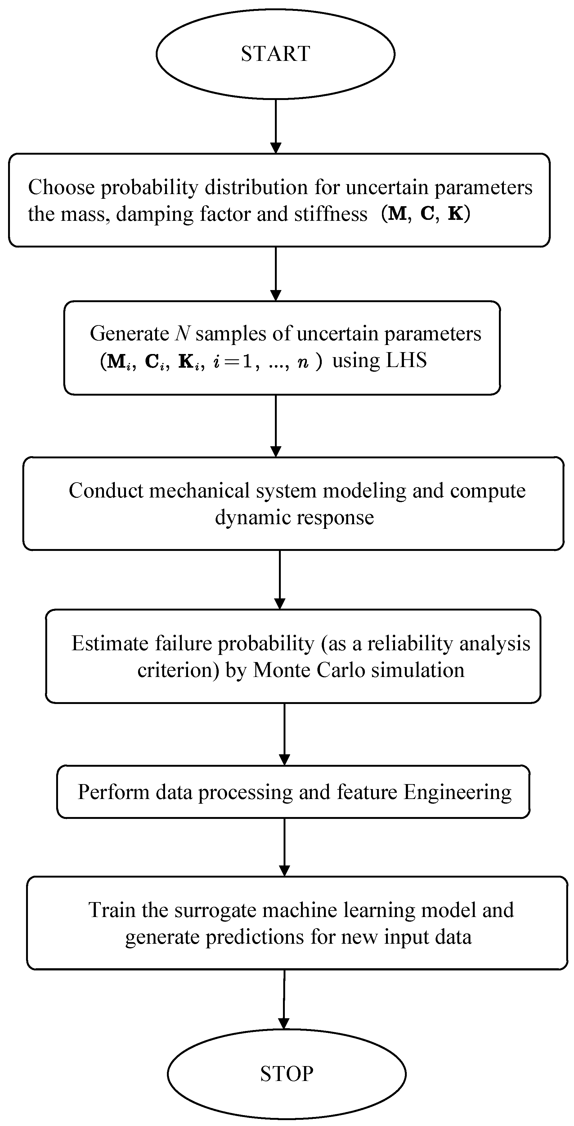
Figure 2.
Multi-degree-of-freedom structural system equipped with TMDs.
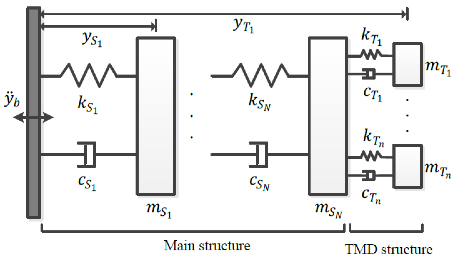
Figure 3.
Performance metrics of the Random Forest model: (a) Correlation Coefficient between predicted and observed values. (b) RMSE representing the average prediction error magnitude.
Figure 3.
Performance metrics of the Random Forest model: (a) Correlation Coefficient between predicted and observed values. (b) RMSE representing the average prediction error magnitude.
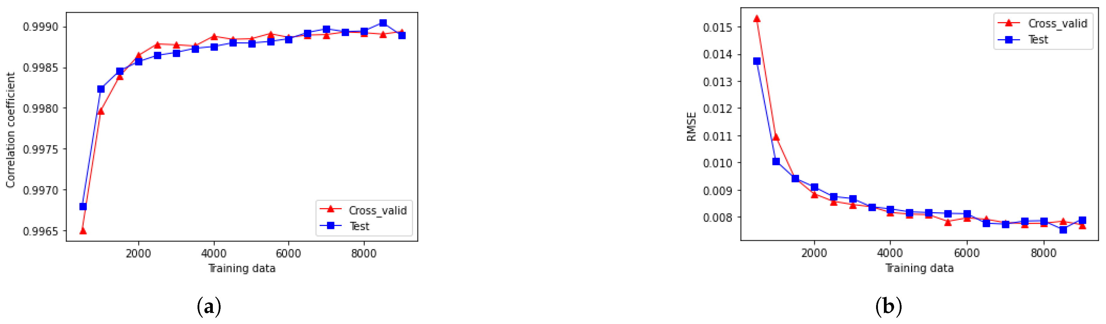
Figure 4.
Performance of various ML algorithms based on the number of features considered.
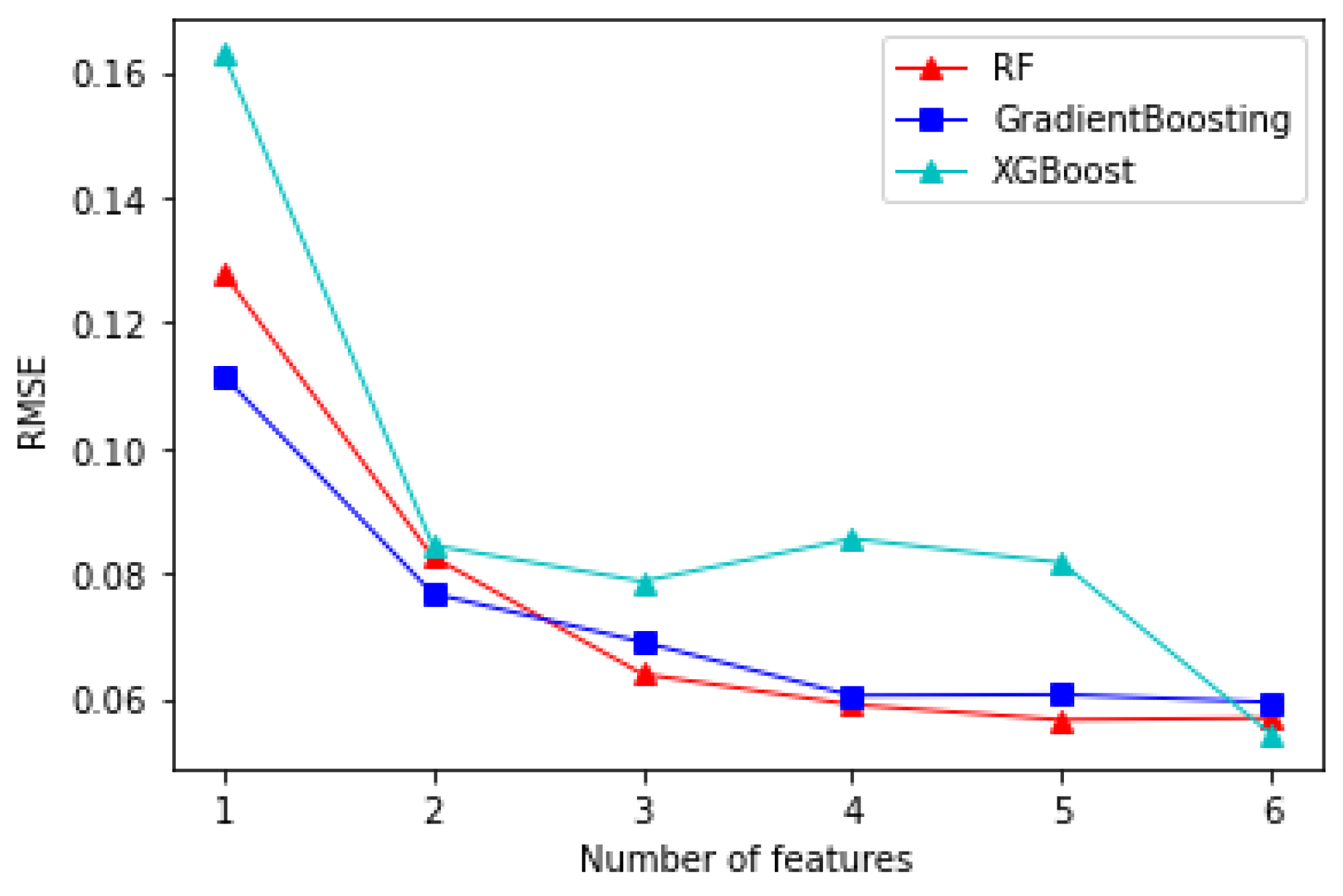
Figure 5.
Scatter plots showing the relationship between tested and predicted values for failure probability across different ML models: (a) Neural Network. (b) Random Forest.(c) Gradient Boosting. (d) Extreme Gradient Boosting.
Figure 5.
Scatter plots showing the relationship between tested and predicted values for failure probability across different ML models: (a) Neural Network. (b) Random Forest.(c) Gradient Boosting. (d) Extreme Gradient Boosting.
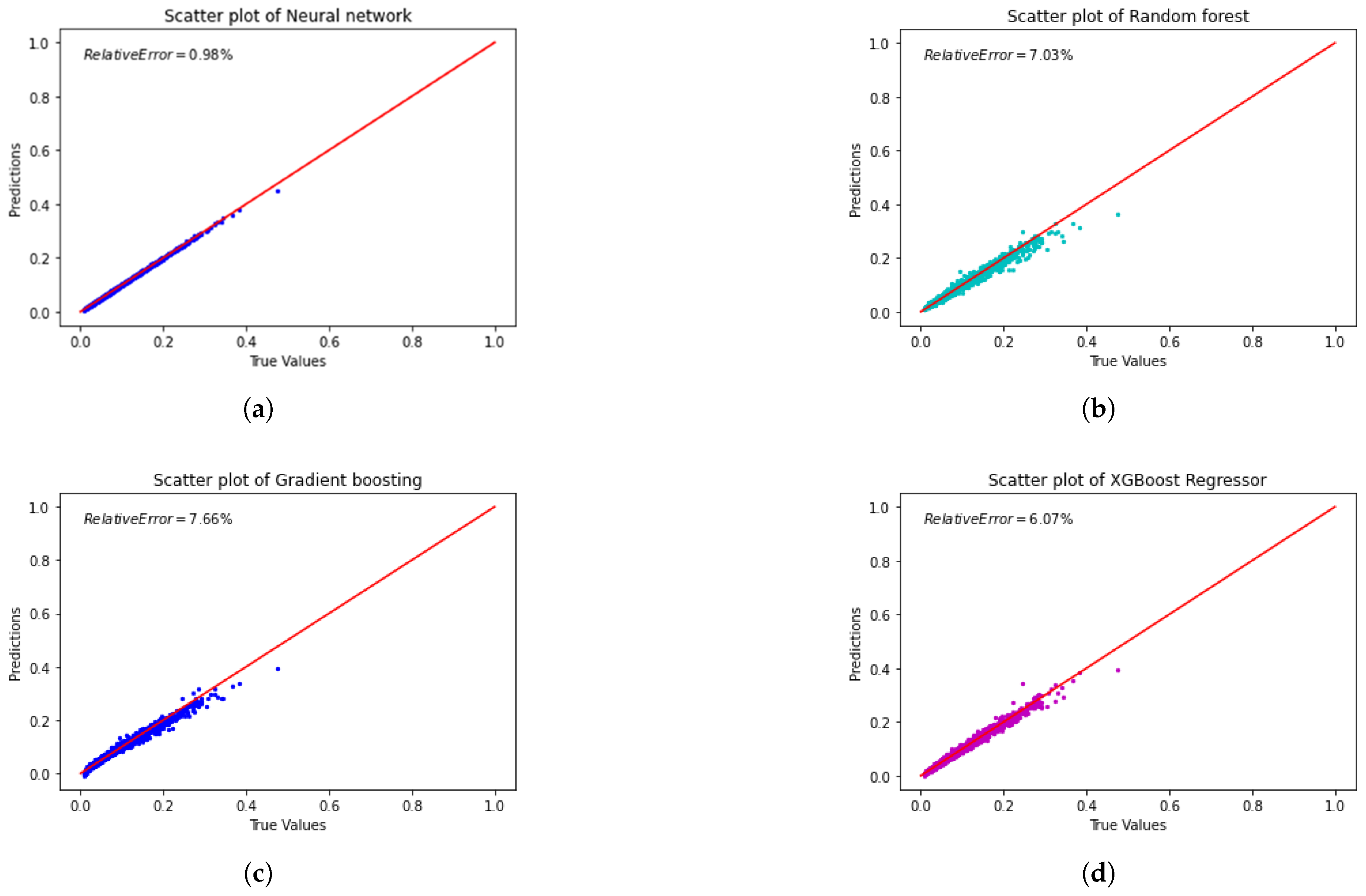
Figure 6.
Feature importance of different mass units.
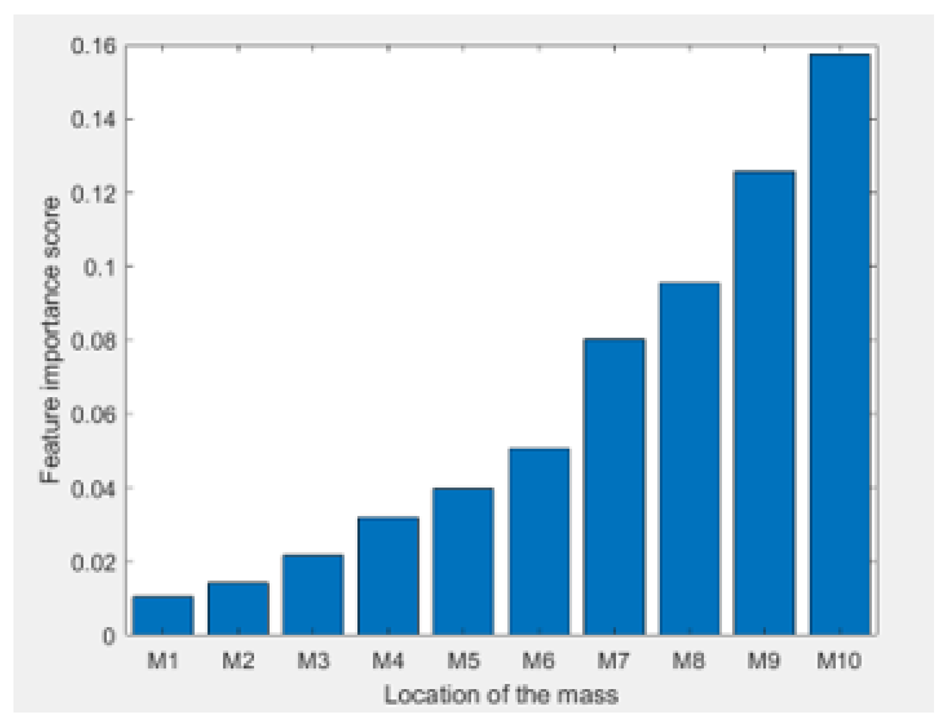
Figure 7.
Plotmatrix of inputs and output, showing the relationship between different parameters.
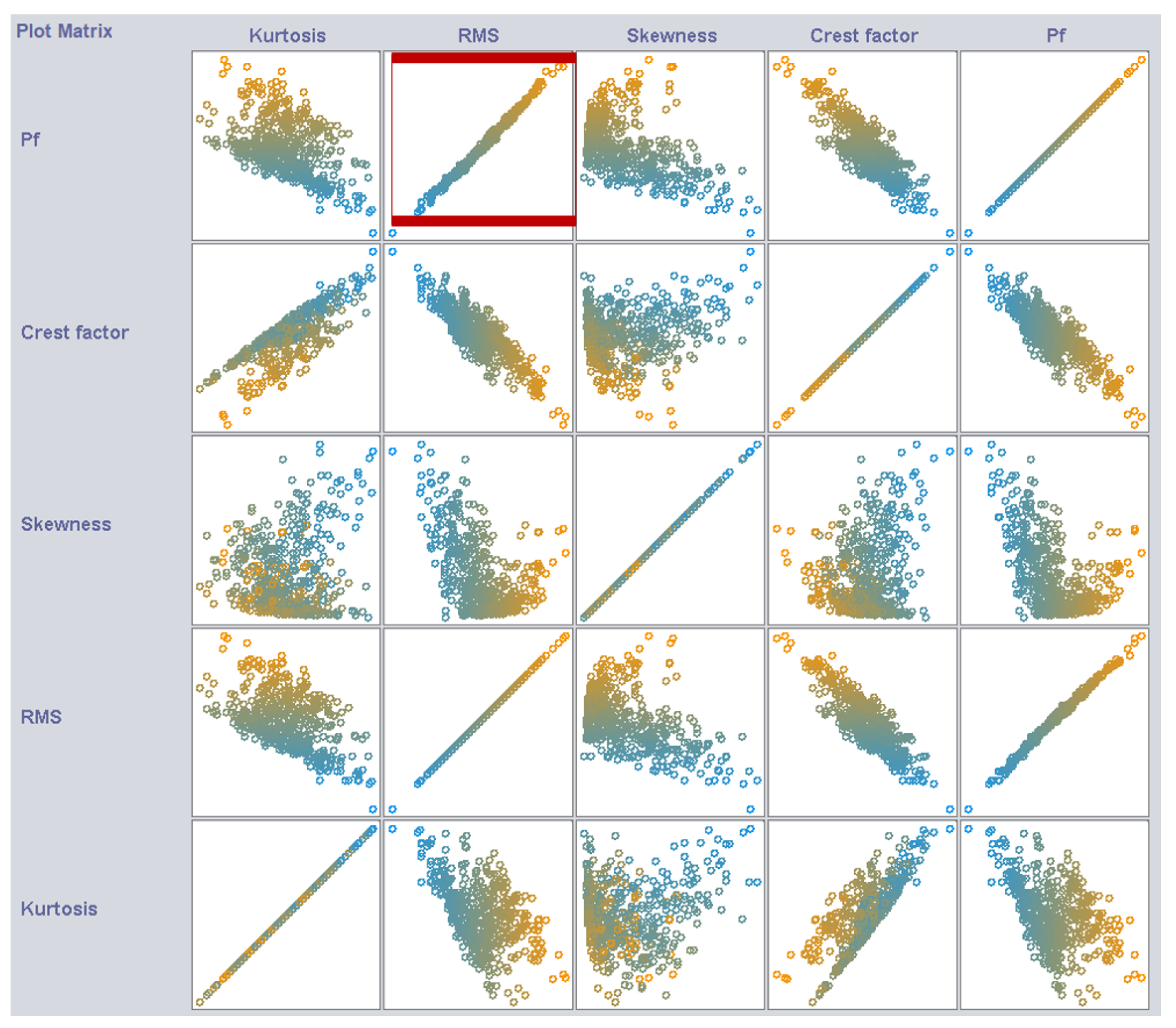
Figure 8.
Scatter plots comparing tested vs. predicted values for failure probability using different ML models.(a) Test vs. Predicted values (Random Forest). (b) Test vs. Predicted values (XGBoost).(c) Test vs. Predicted values (NN)).
Figure 8.
Scatter plots comparing tested vs. predicted values for failure probability using different ML models.(a) Test vs. Predicted values (Random Forest). (b) Test vs. Predicted values (XGBoost).(c) Test vs. Predicted values (NN)).
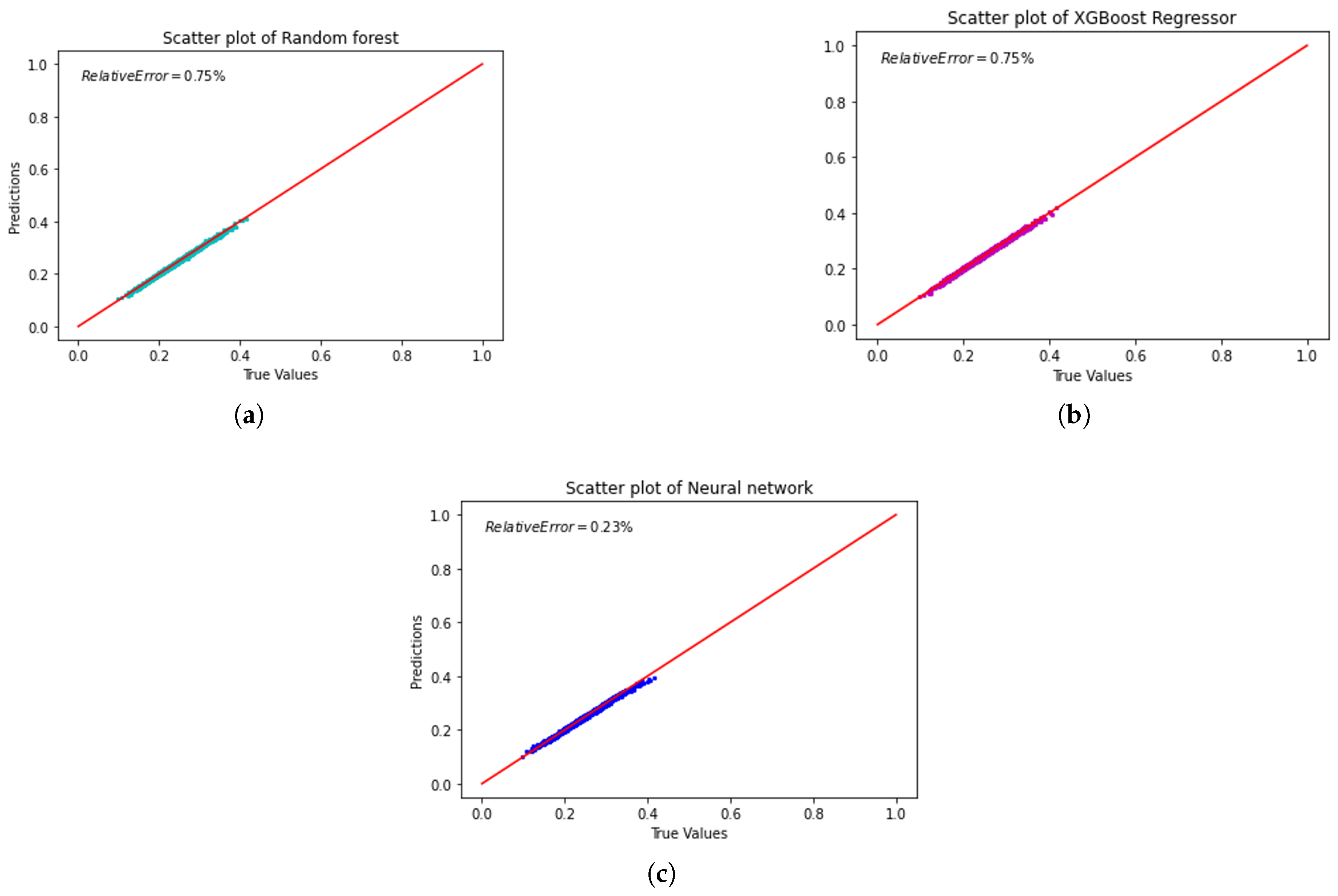

Table 1.
Sample nominal parameters for a 1-DOF TMD system.
| Component | Mass (kg) | Damping (N·s/m) | Stiffness (N/m) |
|---|---|---|---|
| Base structure | 1.0 | 0.03 | 696.4 |
| TMD | 0.02 | 0.0695 | 12.725 |
Table 2.
Comparison of MAE for Different ML Models Across Varying Sample Sizes.
| Sample Size | Random Forest | Gradient Boosting | XGBoost |
|---|---|---|---|
| 2,000 | 0.004830 | 0.004479 | 0.004447 |
| 5,000 | 0.004204 | 0.004013 | 0.003911 |
| 8,000 | 0.003755 | 0.003840 | 0.003819 |
| 10,000 | 0.003763 | 0.003708 | 0.003794 |
Table 3.
Nominal Values of the 2-DOF Structure.
| Parameter | Mass () | Damping () | Stiffness () |
|---|---|---|---|
| 1st DOF | 6 | 62 | 6,500 |
| 2nd DOF | 6 | 62 | 6,500 |
| TMD | 1.38 | 38.997 | 1.8327 |
Table 4.
Comparison of RMSE and MAE for Different ML Models.
| Model | RMSE | MAE |
|---|---|---|
| Random forest | 0.011663 | 0.007297 |
| Gradient boosting | 0.009969 | 0.006335 |
| Xtrem Gradient Boosting | 0.009211 | 0.006150 |
| Neural network | 0.003703 | 0.003264 |
Table 5.
Nominal values of the TMD-based structure.
| Variables | Mean | SD |
|---|---|---|
Disclaimer/Publisher’s Note: The statements, opinions and data contained in all publications are solely those of the individual author(s) and contributor(s) and not of MDPI and/or the editor(s). MDPI and/or the editor(s) disclaim responsibility for any injury to people or property resulting from any ideas, methods, instructions or products referred to in the content. |
© 2025 by the authors. Licensee MDPI, Basel, Switzerland. This article is an open access article distributed under the terms and conditions of the Creative Commons Attribution (CC BY) license (http://creativecommons.org/licenses/by/4.0/).
Copyright: This open access article is published under a Creative Commons CC BY 4.0 license, which permit the free download, distribution, and reuse, provided that the author and preprint are cited in any reuse.


