Submitted:
14 January 2025
Posted:
16 January 2025
You are already at the latest version
Abstract
The limitations of fossil energy sources and environmental concerns have prompted efforts to utilize clean and sustainable energy alternatives. The solid oxide fuel cell operating at intermediate temperatures with ammonia fuel is one of the promising options to replace conventional energy sources. Additionally, employing fuel cell performance prediction methods with high accuracy and speed is critically important. In this research, we first numerically simulate the solid oxide fuel cell using ammonia fuel, considering electrolyte leakage and intermediate operating temperatures. Subsequently, we select the effective input parameters to calculate the fuel cell's performance under various conditions. After generating a sufficient dataset, we apply different machine learning algorithms to predict the objective functions, including power density and maximum temperature of the fuel cell. The results reveal the complexity of predicting the fuel cell's power density compared to its maximum temperature. Furthermore, it was found that the XG Boosting method, with an R² value of 0.99, demonstrates the highest efficiency in predicting the parameters of maximum temperature and power density. It was also observed that the Random Forest and K-Neighbors methods had the lowest accuracy in predicting power density and maximum temperature, respectively, among the eleven methods used.
Keywords:
Solid Oxide Fuel Cell
; Ammonia Fuel
; Electrolyte Leakage
; Intermediate Working Temperature
; Machine Learning
1. Introduction
As the demand for energy rises and concerns about the environment and climate change grow, along with the rising costs and depletion of fossil fuels, research is increasingly focused on clean and sustainable energy sources. The use of fuel cells appears to be a promising approach for utilizing these resources, as suggested by the research findings. Fuel cells have suitable characteristics, including low emissions of pollutants and environmental impacts, low noise, good durability and stability, and high efficiency. The solid oxide fuel cell has garnered increased interest compared to other fuel cell types, attributed to its superior efficiency, versatility with a range of input fuels, adaptability for various scales of application, usability in combined cycles, less sensitivity to impure fuels, and lower catalyst costs. However, the high operating temperature characteristic of conventional solid oxide fuel cells presents numerous challenges, such as efficiency loss over time, thermal stresses, the generation of detrimental compounds like nitrogen oxides, and extended startup durations. Moreover, the utilization of hydrogen as a fuel source within solid oxide fuel cells presents significant challenges. The inherent properties of hydrogen, encompassing its low energy density, the necessity for intricate and costly technologies and infrastructure for both storage and transportation, as well as the potential hazards associated with leakage, have catalyzed the advancement of solid oxide fuel cells that employ alternative fuels and operate at intermediate temperatures (400 to 700 degrees Celsius) in recent years (1,2). Among all chemical compounds, ammonia contains the highest concentration of hydrogen, which can be liquefied and stored under moderate temperature and pressure conditions. This property facilitates its transportation to various locations through multiple methods, including maritime shipping. Furthermore, it used without emitting carbon compounds. The energy density of liquid ammonia is approximately equal to that of fossil fuels and more than twice that of compressed hydrogen gas, positioning it as a viable candidate for application in solid oxide fuel cells. Solid oxide fuel cells with intermediate operating temperatures can effectively use ammonia as a fuel. Ammonia serves as a carbon-free energy carrier, offering superior production and distribution advantages compared to hydrogen. Recent developments indicate that the direct application of ammonia within the fuel cell, along with its thermal decomposition at the anode, is not only practical but also enhances the efficiency of the cell. Furthermore, this approach has the potential to diminish the release of harmful pollutants and mitigate the risk of degradation of cell components (3). To simulate a solid oxide fuel cell with intermediate working temperature and ammonia fuel, it is essential to employ kinetic models that can accurately and efficiently predict the ammonia decomposition reaction process. At low operating temperatures, the hydrogen inhibition phenomenon is significant and affects the process of ammonia decomposition at different hydrogen concentrations. Therefore, the Temkin-Pyzhev kinetic model was employed instead of the Tamara kinetic model, which is a conventional model for high temperatures. This shift in the modeling approach allows for a more accurate representation of the reaction kinetics under the specific temperature conditions encountered in this study. This model has been validated through numerous studies, and its applicability has been substantiated up to a temperature of approximately 660 °C.
In recent years, the application of artificial intelligence subfields, particularly machine learning, has seen significant growth within engineering disciplines. These methodologies can analyze intricate datasets derived from numerical simulations or experimental investigations, thereby identifying patterns and complex interrelationships among various parameters. For instance, in the numerical simulation of a fully porous solid oxide fuel cell operating at intermediate temperature and utilizing ammonia as fuel, numerous factors—including the porosity of the electrolyte and electrodes, operating temperature, chemical and electrochemical reactions, concentrations of different compounds, and pressure—can influence the fuel cell's performance. These factors contribute to nonlinear expressions and complexities within the relationships and equations governing the system. Consequently, the process of solving and calculating key parameters, such as the maximum temperature or power density of the fuel cell, can be both time-consuming and challenging. Under these conditions, the creation of comprehensive and precise data sets encompassing a range of different parameter values can facilitate the training of machine learning models to discern the relationships and computational patterns associated with the target parameter. Subsequently, the trained model can predict the target function across various cases with high accuracy and efficiency (4).
In 2022, Legala et al. conducted a study examining the performance of a polymer fuel cell through the application of two machine learning techniques: artificial neural network and support vector machine. The research utilized two sets of laboratory data and one-dimensional simulation for the machine learning analysis. The input variables considered in the study included current, temperature, reactant pressure, and humidity, while the output variables comprised voltage, resistance, and membrane hydration. The findings indicated that the artificial neural network has superior performance relative to the support vector machine (5). Thereafter, in 2024, Madhavan et al. investigated the performance of machine learning algorithms for predicting the output parameters related to the corrosion current density and impedance of a polymer fuel cell, utilizing the input terms of thickness, contact angle, and voltage. The research assessed the performance of artificial neural networks (ANN) and extreme gradient boosting (XGB) methods, with findings demonstrating that the artificial neural network exhibited superior performance (6). The Finite Gaussian Distribution of Relaxation times method was utilized by Williams et al. (7) to analyze electrochemical impedance spectroscopy data from solid oxide fuel cells with 600°C working temperature. The findings showed that this approach was effective in determining the relationship between electrode voltage and current. In 2023, Vairo et al. (8) studied the safety of fuel cell operations in the shipbuilding and marine industry through numerical simulation and machine learning. To predict the output term, which in this study is the presence of leakage, a boosted-gradient decision tree algorithm with input terms of voltage, electric current, frequency, and internal resistance was employed. The results indicated that the decision tree method was effective in accurately predicting the safe functioning of fuel cells. Tofigh et al. (9) utilized a modified artificial neural network model to predict the transient performance of tubular solid oxide fuel cells. The required dataset was generated through experimental procedures, with key input parameters comprising flow rate, air and fuel flow rates, and operating temperature. The results confirmed that the selected machine learning algorithm achieved high accuracy and computational efficiency in predicting the output voltage of the fuel cell. Rizvandi et al. (10) conducted a numerical analysis of the stack performance of solid oxide fuel cells, assuming ammonia decomposition as the primary source of fuel consumption. Considering the ammonia decomposition endothermic reaction and the temperature drop at the fuel cell inlet, the effects of thermal stress were evaluated. The findings indicated that ammonia decomposition in both direct internal and external modes has a minimal impact of less than five percent on the fuel cell's performance and a lower level of thermal stress was noted in the co-flow mode. In addition, the magnitude of thermal stress exhibits a direct and inverse correlation with the inlet temperature and the velocity of air flow, respectively. In another investigation, Asadi et al. (11) calculated the appropriate values of temperature, pressure, anode and cathode stoichiometry coefficients, and relative humidity through numerical simulation of the of the polymer fuel cell in various flow field states in order to find the highest efficiency. These data used to train the multi-objective optimization (MOO) method to obtain the highest power density value. The performance of fuel cell-battery of Toyota Mirai 2 vehicle was evaluated by Legala et al. (12) with artificial neural network method. In this study, various data were extracted in different modes by surveying the vehicle on the dynamometer chassis, selecting fifteen input features and five output terms. The results illustrated that the optimal network structure for predicting target variables, which incorporates two hidden layers, is the rectified linear unit (ReLU) activation function and adaptive moment estimation (Adam) with coefficient of determination (R-Squared) exceeding 0.98. Pan et al. (13) investigated the operational efficiency of a polymer fuel cell utilizing artificial neural network. In this research, following the identification of influential terms, the requisite training data for machine learning was derived through numerical simulation. The root mean square error (RMSE) was approximately 0.2% according to their findings. Zhou et al. (14) established a laboratory infrastructure dedicated to polymer fuel cells, which enabled the generation of essential data for machine learning applications. They used the long short-term memory (LSTM) method and genetic algorithm to calculate the optimal fuel cell performance conditions. The results showed a coefficient of determination greater than 0.98. The performance of a combined cycle system comprising solid oxide and molten carbonate fuel cells with gasifier and carbon dioxide recovery units was optimized using an artificial neural network by Hai et al. (15). The findings demonstrated the neural network's capability to discern the connection between input and output data, as well as its efficiency in system optimization within a brief timeframe. In another study investigated by Hai et al. (16), the efficiency of solid oxide fuel cell with absorption-ejection refrigeration optimized with three different machine learning algorithms, including support vector machine, decision tree (DT), and artificial neural network. Wang et al. (17) employed machine learning technique coupled with multi-objective genetic algorithms to analyze and enhance the efficiency of a solid oxide fuel cell utilizing methane as the main fuel source. Their investigation involved predicting three output variables: maximum temperature, current density, and carbon deposition. The predicted terms exhibited the coefficient of determination more than 0.97. In 2020, Xu et al. (4) delved into solid oxide fuel cell performance with methane as input fuel by combining deep neural network and numerical simulation. The results demonstrated that all target variables including the heat source, maximum temperature gradient and current density, were predicted with appropriate accuracy. Iskenderoglu et al. (18) utilized two machine learning techniques, namely random forest (RF) and support vector machines, to forecast the output voltage of a solid oxide fuel cell. In this study, the required data for machine learning models was generated in a laboratory setting. Upon evaluation of the models, it was determined that the support vector machine exhibited a higher accuracy in comparison with the random forest method. In the assessment carried out by Lai et al. (19), the thermoelectric performance of methane-fueled solid oxide fuel cell was investigated using multiple linear regression (MLR) and artificial neural networks. The fuel cell power and temperature were predicted by employing the Pearson Correlation Coefficient (PCC) through this study. The findings demonstrated that the neural network approach exhibited a lower error rate of 0.66, in contrast to the multiple linear estimation method, which recorded an error rate of 1.89.
In the current paper, the ammonia-fueled solid oxide fuel cell operating at intermediate temperature is utilized due to ammonia’s unique characteristics, including its suitable energy density and environmental compatibility. This study employs Temkin-Pyzhev kinetic model, while considering the hydrogen inhibition and ammonia decomposition process, to achieve efficient results of electrochemical equations. Subsequently, a numerical simulation is conducted of all porous tubular solid oxide fuel cell with proton conduction, considering ammonia fuel, the Temkin-Pyzhev kinetic model, and the intermediate working temperature. Moreover, the influence of six input variables—namely, operating temperature, electrolyte porosity, anode and cathode characteristics, and the flow rates of fuel and air—on various objective functions, which include power density and both maximum and average temperatures within the fuel cell, is investigated through a parametric study and sensitivity analysis. Finally, the collected data set from numerical simulation is employed to train eight distinct machine learning algorithms, followed by an evaluation of their accuracy in predicting target variables.
2. Materials and Methods
In this study, the model geometry is simulated in a two-dimensional axisymmetric form. The ammonia fuel and air enter the fuel cell through the innermost and outermost channels, respectively. The chemical reaction of ammonia decomposition occurs within the anode, where hydrogen is generated to provide the electrochemical reaction and proton production. Subsequently, the proton moves through the electrolyte and reaches the cathode, where water is generated during the oxidation reaction. The porous nature of the electrolyte allows various species to pass through. Figure 1 illustrates the model geometry in two and three dimensions (20).
Figure 2 provides a two-dimensional representation of the problem's geometry, highlighting the species involved in both chemical and electrochemical reactions. It illustrates how these species flow in through the fuel and air channels, with the potential to traverse different sections of the fuel cell. Additionally, Figure 2 depicts the chemical reaction associated with ammonia decomposition occurring in the anode area.
Table 1 shows the sizes of the various parts of the fuel cell.
The ammonia Fuelled SOFC operates in the temperature range of 400 to 700 degrees Celsius. Therefore, the application of the Temkin-Pyzhev kinetic model, which incorporates the phenomenon of hydrogen inhibition, is deemed suitable for the decomposition of ammonia. This model is represented in Equation (1) [1].
In Equation (1), the expressions , , and are the rates of the chemical reaction of ammonia decomposition, the partial pressures of ammonia and hydrogen, respectively. Additionally, R and T denote the universal gas constant and temperature, respectively.
2.1. Governing Equations
To numerically simulate and assess the performance of a fuel cell, it is essential to identify, define, and solve the governing equations. As previously noted, different species within the fuel and air flows enter the fuel cell at specific velocities and temperatures. After moving and penetrating the electrodes, these species engage in chemical and electrochemical reactions that generate electric current. In this context, the conservation equations for mass, momentum, species, electric flux, and energy are established, along with an explanation of the relevant assumptions (21,22).
2.1.1. Flow Field
The analysis of the velocity and pressure distributions of fuel and air flows within channels is carried out using the mass and momentum conservation equations. These equations are applied under the conditions of laminar and compressible flow (with a Mach number below 0.3) and are considered in a steady-state context, as outlined in Equations (2) and (3) (23).
In the above equations, the quantities V, , p and μ are the velocity field, density, pressure field, and dynamic viscosity of the fluid flow, respectively. The variable denotes the mass produced or consumed per unit volume, which is used in electrodes according to chemical and electrochemical reactions and has a value of zero in channels and electrolytes.
The Darcy-Brinkman equation is employed to analyze flows in porous media, such as electrodes and electrolytes, by considering the impact of porosity on velocity and pressure fields as follows:
In Equation (4), the terms and κ are the porosity of the medium and the permeability coefficient, respectively.
2.1.2. Species
The fuel and air flows are gaseous mixtures containing hydrogen, nitrogen, water vapor, and ammonia species that are produced or consumed in the anode and cathode sections of the fuel cell. These species are transported through two mechanisms: diffusion and accumulation. The mole fraction of each species at various locations is computed using the Stefan-Maxwell conservation equation, represented in Equation 5.
and are the infiltration mass flux and volume fraction of each species, respectively. also represents the production or consumption of each species in terms of moles per unit volume.
Symbols , , , , , and represent Infiltration driving factor, effective binary diffusion coefficient, effective transfer factor, binary diffusion coefficient, molar fraction of species, average molar mass and molar mass of species, respectively.
2.1.3. Electric Flux
Through the oxidation reaction occurring at the anode, hydrogen gas is transformed into protons. The movement of these protons and electrons through the electrolyte and the external circuit generates ionic and electrical currents. Equations (9) and (10) illustrate the electrochemical oxidation and reduction reactions that take place at the fuel cell's anode and cathode, respectively.
Conservation of flux (Ohm's law) is used to investigate and analyze ionic and electrical currents in the electrolyte, anode, and cathode as follows:
In the above relations, , , and represent the electronic and ionic conductivities and the electronic and ionic potentials, respectively. The quantity determines the current produced or consumed in the fuel cell. The Butler-Volmer equation is employed to ascertain the connection between the current and the excess activation potential.
, , , , F and η are the electrochemical active surface area of the porous electrode per unit volume, exchange current density, anodic and cathodic charge transfer coefficient, Faraday constant and excess activation potential, respectively. The variables and represent the ratios of reduced and oxidized species in relation to their respective reference values.
The excess activation potential (η) is defined as follows:
is the open circuit potential, which is zero at the anode and is determined as follows at the cathode:
2.1.4. Energy
Considering the importance and influence of temperature on fuel cell performance, alongside the endothermic nature of ammonia decomposition, the energy conservation equation is utilized to determine the temperature distribution within a fuel cell.
Under the assumption of local thermal equilibrium, it is considered that the temperature of both the fluid and solid phases within the porous medium is identical. For the fluid flow (perfect gas) in the fuel and air channels, the specific heat capacity and average molar mass are determined based on temperature, pressure, and the mole fraction of the gas mixture components. Effective thermal conductivity is then applied to compute the temperature distribution in the porous media, which encompasses both the electrodes and the electrolyte. In Equation 16, , T, and are the specific heat capacity, temperature, heat source or sink resulting from chemical and electrochemical reactions and effective thermal conductivity, respectively. is defined as follows:
The heat source includes the heat produced or consumed in different parts of the fuel cell, which is defined as Equation 18.
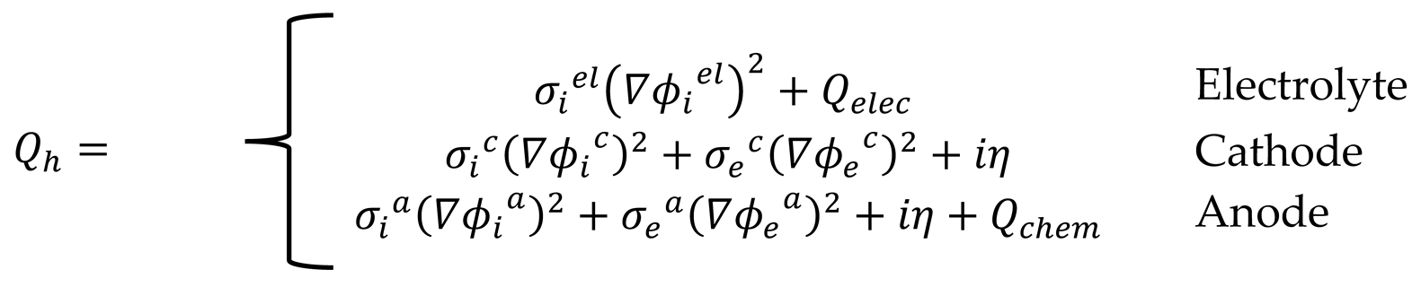
, , iη and are the heat source from electrochemical reactions, ohmic heat loss, excess potential heat dissipation and chemical reaction from ammonia decomposition, respectively. The thermal enthalpy of the endothermic reaction of ammonia decomposition is 46 kJ/mol.
2.2. Validation
In this section, the accuracy and precision of the numerical solution is examined with the research of Ranasinghe et al. (24). In Figure 2, the power density-current density changes in the two studies are compared, which indicates the appropriate accuracy of the solution method used in this study.
To predict target parameters using machine learning algorithms, a sufficient dataset is essential. Therefore, in the initial phase, six key input variables are identified: anode porosity, cathode porosity, electrolyte porosity, inlet temperature, fuel flow rate, and air flow rate. Subsequently, by varying these input parameters within a specific range, the resulting values for the target functions—such as power density, maximum temperature, and average temperature of the fuel cell—are determined.
3. Data Analysis
Following the simulation of a proton solid oxide fuel cell operating at an average temperature using ammonia fuel, the impact of different input parameters on the fuel cell's performance is analyzed while maintaining other variables constant. By varying the input parameters within a relevant range, the target parameters are calculated. Figure 4 illustrates the changes in power density in relation to the input parameters.
Figure 1.
Effect of changing input parameters on power density.
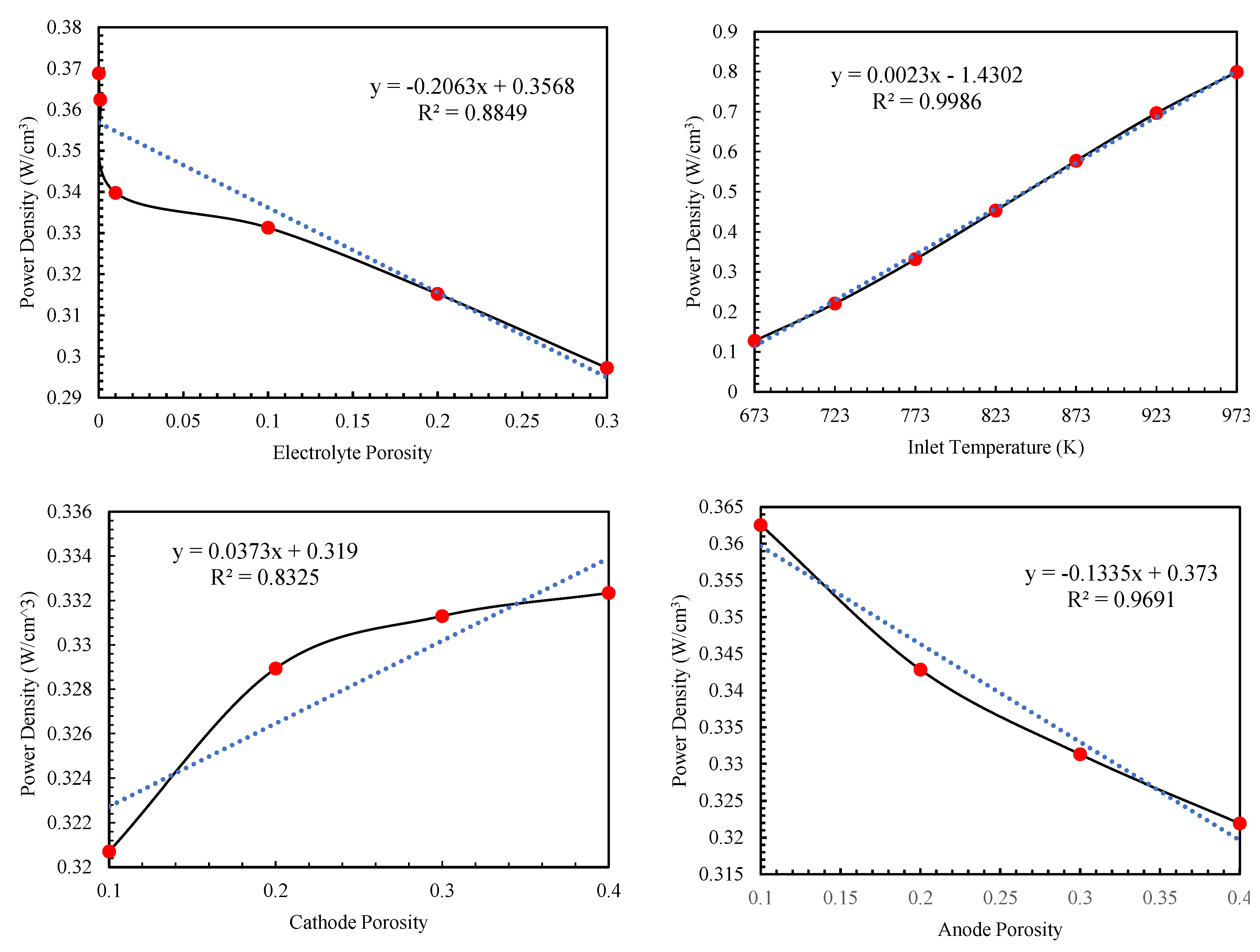
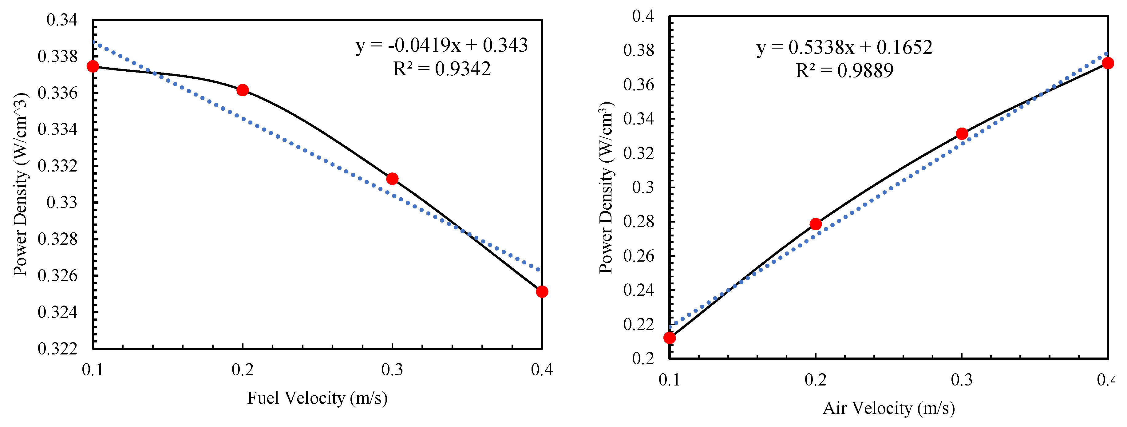
The simulation and resolution of the equations are conducted at a voltage of 0.7 V, an inlet temperature of 773 Kelvin, and an electrolyte porosity of 0.1. Additionally, the porosity and flow velocity are set at 0.3 and 0.3 m/s, respectively. As illustrated in Figure 4, an increase in electrolyte porosity leads to a decline in fuel cell performance. The power density experiences a more significant decrease at porosity values below 0.01, with an 8% reduction when porosity increases from 0.0001 to 0.01 and a 20% reduction when it rises to 0.3. Conversely, the power density of the fuel cell increases linearly as inlet temperature grows, demonstrating a predictable relationship with accurate estimation. For instance, the power density rises from 0.22 at 673 K to 0.8 at 973 K as the temperature increases. However, increasing the porosity of the anode and cathode electrodes negatively impacts the fuel cell’s performance. Increasing the anode porosity reduces the power density of the fuel cell. As can be seen in Figure 4, this decreasing trend can be predicted with a good approximation in a linear manner. Increasing the porosity of the cathode enhances the performance of the fuel cell, exhibiting a gradual and nonlinear slope, in contrast to the influence of the anode. Additionally, as displayed in Figure 4, the impact of anode porosity is significant and surpasses that of cathode porosity. Increasing the fuel and air flow rates have an inverse effect on the performance of fuel cells and a rise in the air flow rate correlates with an almost linear increase in the fuel cell's power density. For instance, boosting the air flow from 0.1 to 0.4 results in approximately a 76% increase in power density. Conversely, raising the ammonia flow rate, which serves as the input fuel, negatively impacts the fuel cell's power output. However, this negative effect is less pronounced compared to other factors; for example, an increase in fuel flow from 0.1 to 0.4 leads to a reduction in power density by 3.6%.
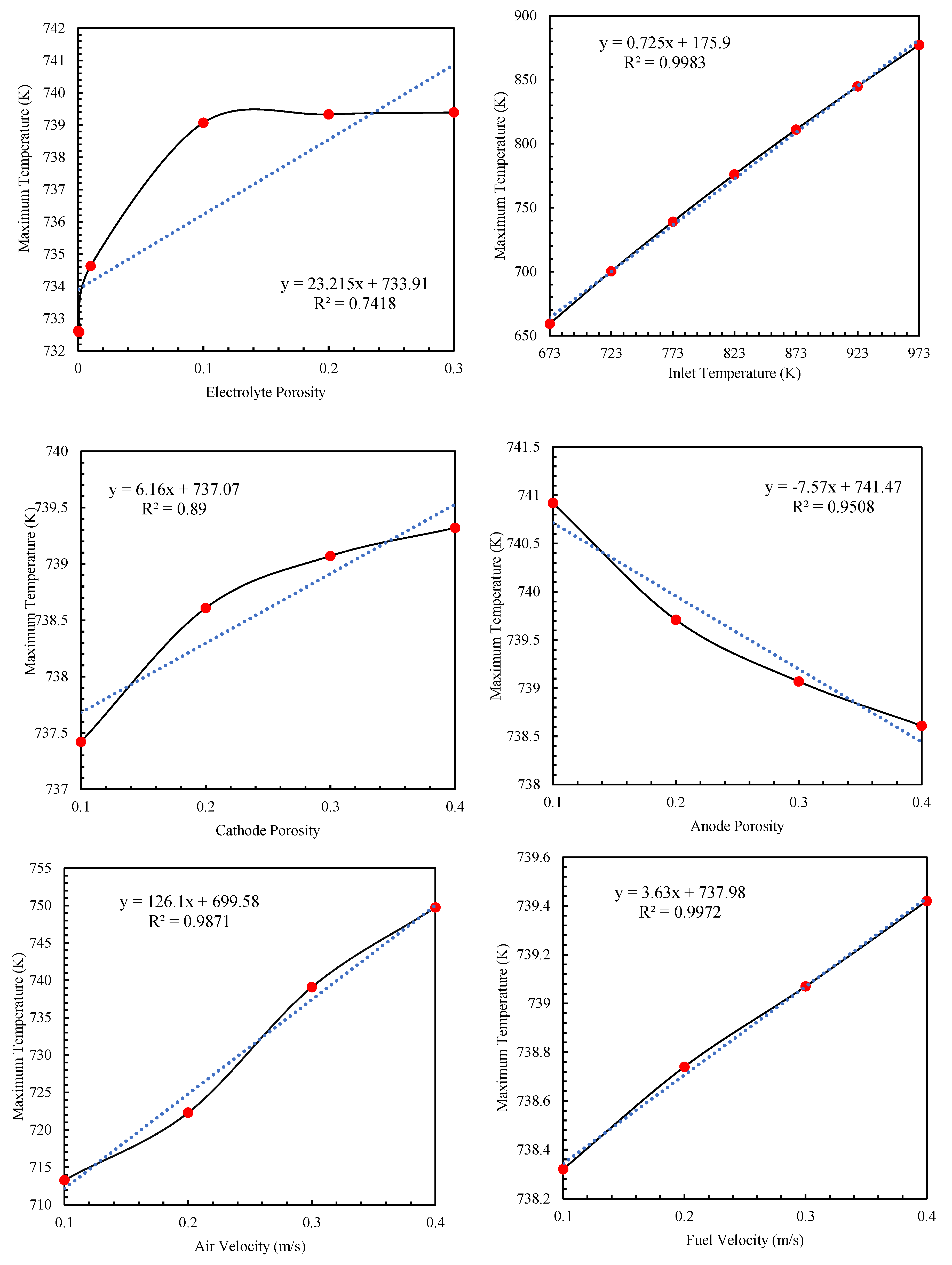
Figure 5 shows the impact of the selected input parameters on the targeted variables, which encompass the fuel cell's maximum temperature and power density. Augmentation of electrolyte porosity leads to a slight elevation in the maximum temperature of the fuel cell, approximately 0.1. However, further increases in porosity do not result in any notable alteration in the maximum temperature. Moreover, the fluctuations observed in the graph signify a non-linear pattern in the correlation between maximum temperature and the rise in electrolyte porosity. Increasing the porosity of the fuel cell from 0.0001 to 0.1 results in an approximate eight-degree increase in the maximum temperature of the fuel cell. Regarding the effect of inlet temperature, as expected, a direct relationship is observed between the maximum temperature and the fuel cell inlet temperature. The alterations in the diagram of maximum temperature and inlet temperature indicate a linear correlation between the two variables with reasonable accuracy. Figure 5 highlights the differing effects of porosity on the maximum temperature of the anode compared to the cathode. Elevating the anode's porosity leads to a linear decrease in the fuel cell's maximum temperature, with a reduction of two degrees when porosity rises from 0.1 to 0.4. In contrast, changes in the cathode's porosity have a significantly different effect, resulting in a temperature increase. An increase in cathode porosity from 0.1 to 0.4 causes an increase in temperature by two degrees in a nonlinear trend. Furthermore, Figure 5 demonstrates a clear relationship between the flow rates of fuel and air and the maximum temperature attained by the fuel cell. Adjusting the fuel flow rate from 0.1 to 0.4 raises the maximum temperature by two degrees, while a similar increase in the air flow rate from 0.1 to 0.4 leads to an approximate 32-degree temperature rise.
Figure 4.
Effect of changing input parameters on maximum temperature.
3.1. Correlation Between Data
After generating the input expressions and conducting the calculations, 1,030 data points are generated. Before utilizing this data for machine training, essential processing steps must be undertaken. Initially, the influence of each data point on the others is assessed using the Pearson correlation method. Figure 5 illustrates these effects as reflected in the Pearson Correlation coefficient. As can be seen, the input temperature has the greatest effect and is directly related to the power density of the fuel cell. Additionally, Figure 5 indicates that factors such as porosity or leakage in the electrolyte, as well as a high fuel flow rate, negatively affect the fuel cell's performance.
Table 2 presents the statistical status of the data prior to the preprocessing and preparation phase for machine training. The table includes all calculations of applicable values for solid oxide fuel cell.
To reduce the impact of data arrangement on machine learning, the data is initially shuffled. Once the values are rearranged, it is essential to divide the dataset into training and testing subsets. Specifically, 80% of the data (824 numbers) is allocated for training the machine, while the remaining 20% (206 numbers) is designated for testing.
After separating the data for training and testing the machine, the next step involves data preprocessing. The training data undergoes a standardization process, which serves as a preprocessing technique to normalize all input variables within the dataset. Standardization transforms the data in such a way that each term has a mean of zero and a standard deviation of one. This procedure is crucial for various machine learning algorithms that are sensitive to the scale of input features.
In the equation provided, and denote the different values and the average of each input variable, respectively. Following the computation of the average for each variable, its standard deviation is then determined using Equation 20 as shown below.
represents the standard deviation of each input variable. Following the computation of the average and standard deviation for every input term utilized in machine training, the fitting procedure is conducted. Once fitting is complete, the transformation process of the resulting data takes place, following the Equation 21.
The value of each input term j that has been standardized is denoted by . Additionally, it is essential to apply the transformation process to the data used to evaluate the machine's performance. The fitting process is performed only on the training data to ensure that the machine is not trained on the data used for testing. Following the preprocessing of the data, the machine can proceed to training. Ten machine learning algorithms are employed for this purpose and subsequently assessed for their performance.
4. Results and Discussion
Once the machine has been trained using different algorithms, it undergoes evaluation and testing. For this assessment, the mean absolute error (MAE) and root mean square error (RMSE) criteria are utilized. After predicting the fuel cell's performance with the trained machine, the discrepancies between the predicted values and the actual values are calculated to determine the validity of the machine's performance.
As shown in Table 3, based on the R2 index, the XG Boosting, Gradient Boosting, Random Forest, and Decision Tree algorithms have the best performance in predicting the power density of the fuel cell, respectively. Accordingly, the R2 of the mentioned algorithms is more than 0.99.
Table 4 demonstrates the machine's performance in predicting the maximum temperature of the fuel cell. Notably, the XG Boosting, Decision Tree, Random Forest, Support Vector Machine, and Gradient Boosting algorithms demonstrate optimal performance, with R² values exceeding 0.99.
Comparing the data in Table 3 and Table 4 indicates that the algorithms exhibit greater accuracy in predicting maximum temperature than in forecasting power density. This accuracy improvement is particularly pronounced in the Support Vector Machine algorithm. Accordingly, the R2 of the machine in predicting the power density and maximum temperature is 0.88 and 0.99, respectively. This discrepancy may be attributed to the more linear trend observed in maximum temperature changes in relation to the input parameters, especially the input temperature.
Figure 7 compares the performance of the Support Vector Machine and XG Boosting algorithms. The figure displays both the predicted and actual data, illustrating a strong and acceptable fit for the XG Boosting algorithm in comparison to the Support Vector Machine. High prediction accuracy is reflected in the proximity of the points to the Y=X line, while the deviation from this line signifies a substantial difference between the actual and predicted values.
Figure 8 displays a comparison of the performance of XG Boosting and K Neighbors in predicting the maximum temperature of a fuel cell. The data indicates that the accuracy of maximum temperature predictions is generally better across various algorithms when compared to predictions for power density. While K Neighbors demonstrates lower accuracy relative to the other algorithms, it still achieves an R² value of 0.94.
5. Conclusions
In this study, a solid oxide fuel cell utilizing ammonia fuel, with considerations for electrolyte leakage and average operating temperature, was initially simulated in a tubular (symmetric) configuration. Following the validation of the numerical solution method, key input parameters—such as electrolyte and electrode porosity, fuel and air flow rates, and input temperature—were selected for calculating the objective functions, which included the maximum temperature and power density of the fuel cell. A data set was then generated by varying the input parameters, resulting in 1,030 values, which was used for machine training. Eighty percent of this data was allocated for training the machine with eleven different algorithms, while the remaining twenty percent was utilized for performance evaluation of the trained models. The key findings are outlined below:
- By employing the Pearson correlation coefficient, it was found that the inlet temperature has the most significant influence on the objective functions. Additionally, the analysis revealed that the impact of inlet temperature on the maximum temperature is greater than its effect on the fuel cell's power density.
- The input variables of electrolyte porosity and flow rate exhibit an inverse relationship with power density. Consequently, an increase in either the fuel flow rate or electrolyte porosity is expected to lead to a more pronounced decline in fuel cell performance in comparison to other input parameters.
- The inlet temperature exhibits a direct relationship and has the most substantial impact on the maximum temperature of the fuel cell. In addition, the fuel flow rate shows an inverse relationship and has a significant effect on the maximum temperature in comparison to other input parameters.
- The efficacy of various algorithms in forecasting power density and maximum temperature differs from each other. Accordingly, the XG Boosting algorithm demonstrates the highest accuracy in predicting power density, while the Support Vector Machine algorithm shows the lowest accuracy in this regard.
- The performance of all algorithms deployed in training and testing the machine for predicting maximum temperature is satisfactory, with R² values exceeding 0.9. Consequently, XG Boosting demonstrates the highest accuracy in these predictions, while K Neighbors exhibits the lowest accuracy.
Author Contributions
Conceptualization, methodology, software, validation, formal analysis, investigation, resources, data curation, writing—original draft preparation, writing—review and editing, visualization, M.K.; supervision, M.G. All authors have read and agreed to the published version of the manuscript.
Funding
This research received no external funding.
Data Availability Statement
Data sharing is not applicable.
Conflicts of Interest
The authors declare no conflicts of interest.
References
- Cheddie, DF. Temkin-Pyzhev Kinetics in Intermediate Temperature Ammonia-Fed Solid Oxide Fuel Cells (SOFCs). Int J Power Energy Res [Internet]. [cited 2024 Dec 6] Available from: https://www.researchgate.net/publication/327469802_Temkin-Pyzhev_Kinetics_in_Intermediate_Temperature_Ammonia-Fed_Solid_Oxide_Fuel_Cells_SOFCs. 2018, 2. (accessed on null). [Google Scholar] [CrossRef]
- Ilbas M, Alemu MA, Cimen FM. Comparative performance analysis of a direct ammonia-fuelled anode supported flat tubular solid oxide fuel cell: A 3D numerical study. Int J Hydrogen Energy. 2022, 47, 3416–28. [Google Scholar] [CrossRef]
- Jeerh G, Zhang M, Tao S. Recent progress in ammonia fuel cells and their potential applications. J Mater Chem A [Internet]. [cited 2024 Dec 6]. Available from: https://pubs.rsc.org/en/content/articlehtml/2021/ta/d0ta08810b. 2021, 727–52.
- Xu H, Ma J, Tan P, Chen B, Wu Z, Zhang Y, et al. Towards online optimisation of solid oxide fuel cell performance: Combining deep learning with multi-physics simulation. Energy AI. 2020, 1, 100003. [Google Scholar] [CrossRef]
- Legala A, Zhao J, Li X. Machine learning modeling for proton exchange membrane fuel cell performance. Energy AI. 2022, 10, 100183. [Google Scholar] [CrossRef]
- Madhavan PV, Shahgaldi S, Li X. Modelling Anti-Corrosion Coating Performance of Metallic Bipolar Plates for PEM Fuel Cells: A Machine Learning Approach. Energy AI. 2024, 17, 100391. [Google Scholar] [CrossRef]
- Williams NJ, Osborne C, Seymour ID, Bazant MZ, Skinner SJ. Application of finite Gaussian process distribution of relaxation times on SOFC electrodes. Electrochem commun. 2023, 149, 107458. [Google Scholar] [CrossRef]
- Vairo T, Cademartori D, Clematis D, Carpanese MP, Fabiano B. Solid oxide fuel cells for shipping: A machine learning model for early detection of hazardous system deviations. Process Saf Environ Prot. 2023, 172, 184–94. [Google Scholar] [CrossRef]
- Tofigh M, Salehi Z, Kharazmi A, Smith DJ, Hanifi AR, Koch CR, et al. Transient modeling of a solid oxide fuel cell using an efficient deep learning HY-CNN-NARX paradigm. J Power Sources. 2024, 606, 234555. [Google Scholar] [CrossRef]
- Rizvandi OB, Nemati A, Nami H, Hendriksen PV, Frandsen HL. Numerical performance analysis of solid oxide fuel cell stacks with internal ammonia cracking. Int J Hydrogen Energy. 2023, 48, 35723–43. [Google Scholar] [CrossRef]
- Asadi MR, Ghasabehi M, Ghanbari S, Shams M. The optimization of an innovative interdigitated flow field proton exchange membrane fuel cell by using artificial intelligence. Energy. 2024, 290, 130131. [Google Scholar] [CrossRef]
- Legala A, Kubesh M, Chundru VR, Conway G, Li X. Machine learning modeling for fuel cell-battery hybrid power system dynamics in a Toyota Mirai 2 vehicle under various drive cycles. Energy AI. 2024, 17, 100415. [Google Scholar] [CrossRef]
- Pan Y, Ruan H, Wu B, Regmi YN, Wang H, Brandon NP. A machine learning driven 3D+1D model for efficient characterization of proton exchange membrane fuel cells. Energy AI. 2024, 17, 100397. [Google Scholar] [CrossRef]
- Zhou F, Sun C, Pu J, Li J, Li Y, Xie Q, et al. Efficiency optimization of fuel cell systems with energy recovery: An integrated approach based on modeling, machine learning, and genetic algorithm. J Power Sources. 2024, 615.
- Hai T, Alenizi FA, Ubeid MH, Goyal V, Alhomayani FM, Mohammed Metwally AS. Using machine learning for comparative optimizing a novel integration of molten carbonate and solid oxide fuel cells with CO2 recovering and gasification. Int J Hydrogen Energy. 2023, 48, 38454–72. [Google Scholar] [CrossRef]
- Hai T, Alenizi FA, Mohammed AH, Goyal V, Marjan RK, Quzwain K, et al. Solid oxide fuel cell energy system with absorption-ejection refrigeration optimized using a neural network with multiple objectives. Int J Hydrogen Energy. 2024, 52, 954–72. [Google Scholar] [CrossRef]
- Wang Y, Wu C, Zhao S, Wang J, Zu B, Han M, et al. Coupling deep learning and multi-objective genetic algorithms to achieve high performance and durability of direct internal reforming solid oxide fuel cell. Appl Energy. 2022, 315, 119046. [Google Scholar] [CrossRef]
- İskenderoğlu FC, Baltacioğlu MK, Demir MH, Baldinelli A, Barelli L, Bidini G. Comparison of support vector regression and random forest algorithms for estimating the SOFC output voltage by considering hydrogen flow rates. Int J Hydrogen Energy. 2020, 45, 35023–38. [Google Scholar] [CrossRef]
- Lai M, Zhang D, Li Y, Wu X, Li X. Application of Multiple Linear Regression and Artificial Neural Networks in Analyses and Predictions of the Thermoelectric Performance of Solid Oxide Fuel Cell Systems. Energies [cited 2024 Dec 6]. Available from: https://www.mdpi.com/1996-1073/17/16/4084/htm. 2024, 17, 4084. [Google Scholar] [CrossRef]
- Keyhanpour M, Ghasemi M, Pourbagian M. Parametric Study of Ammonia-Fueled Tubular AP-SOFC with Temkin-Pyzhev Kinetic Model. Iran Chem Eng J. 2023, 22, 98–123. [Google Scholar]
- Keyhanpour M, Ghasemi M. 3D Investigation of Tubular PEM Fuel Cell Performance Assuming Fluid- Solid- Heat Interaction. J Comput Methods Eng. 2022, 41, 79–99. [Google Scholar]
- Keyhanpour M, Ghasemi M. 3D Simulation of Effect of Geometry and Temperature Distribution on SOFC Performance. Fluid Mech Aerodyn [Internet]. Available from: https://fma.ihu.ac.ir/article_206906_en.html. 2022, 10, 169–84.
- Sayadian S, Ghassemi M, Ahmadi S, Robinson AJ. Numerical analysis of transport phenomena in solid oxide fuel cell gas channels. Fuel. 2022, 311, 122557. [Google Scholar] [CrossRef]
- Ranasinghe S, International PM-2017 I, 2017 undefined. Modelling of single cell solid oxide fuel cells using COMSOL multiphysics. ieeexplore.ieee.orgSN Ranasinghe, PH Middleton2017 IEEE Int Conf Environ Electr 2017•ieeexplore.ieee.org [Internet]. [cited 2024 Dec 6]; Available from: https://ieeexplore.ieee.org/abstract/document/7977790/.
Figure 1.
Configuration of 3D tubular SOFC a) front view b) layers.
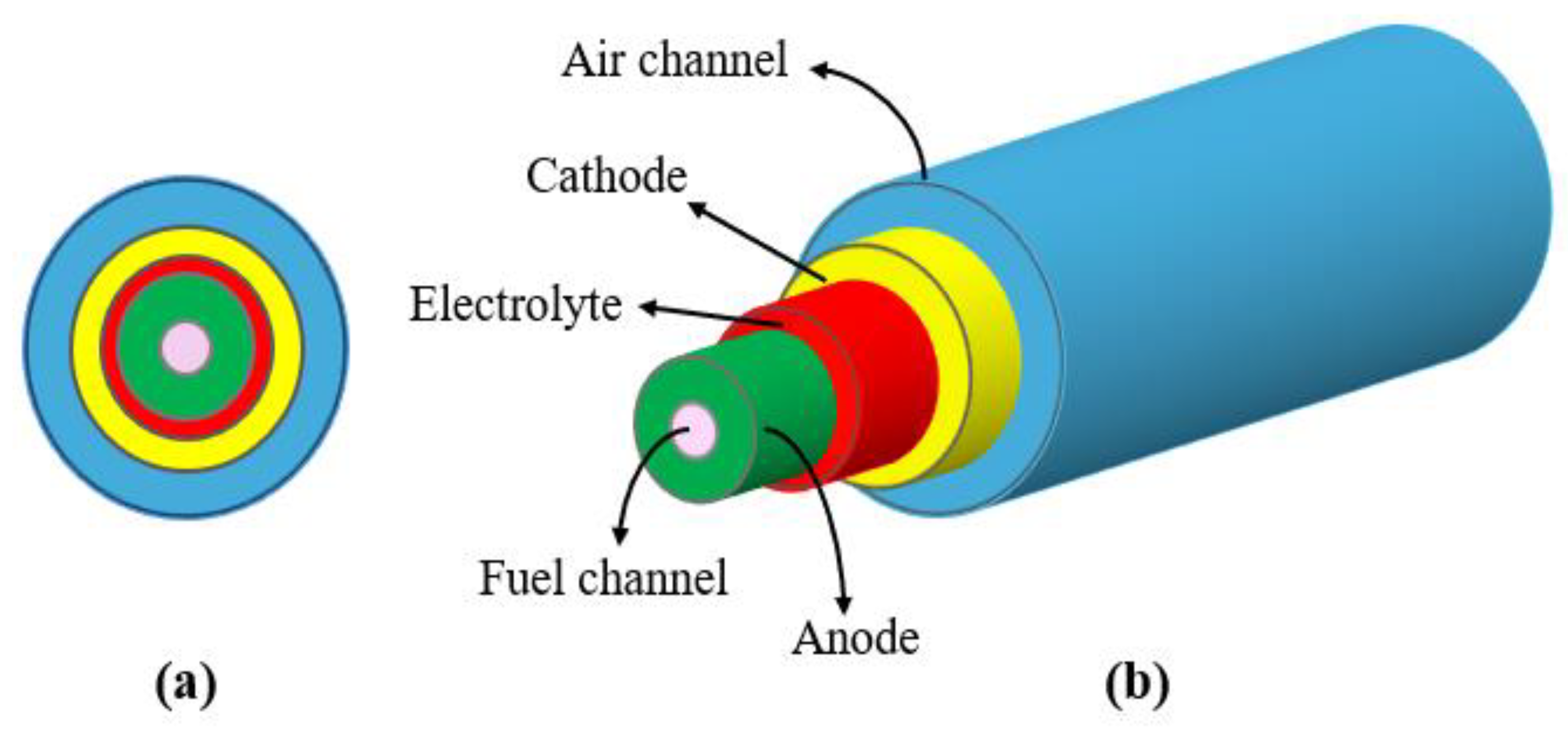
Figure 2.
2D view of SOFC ammonia Fuelled with chemical and electrochemical reactions.
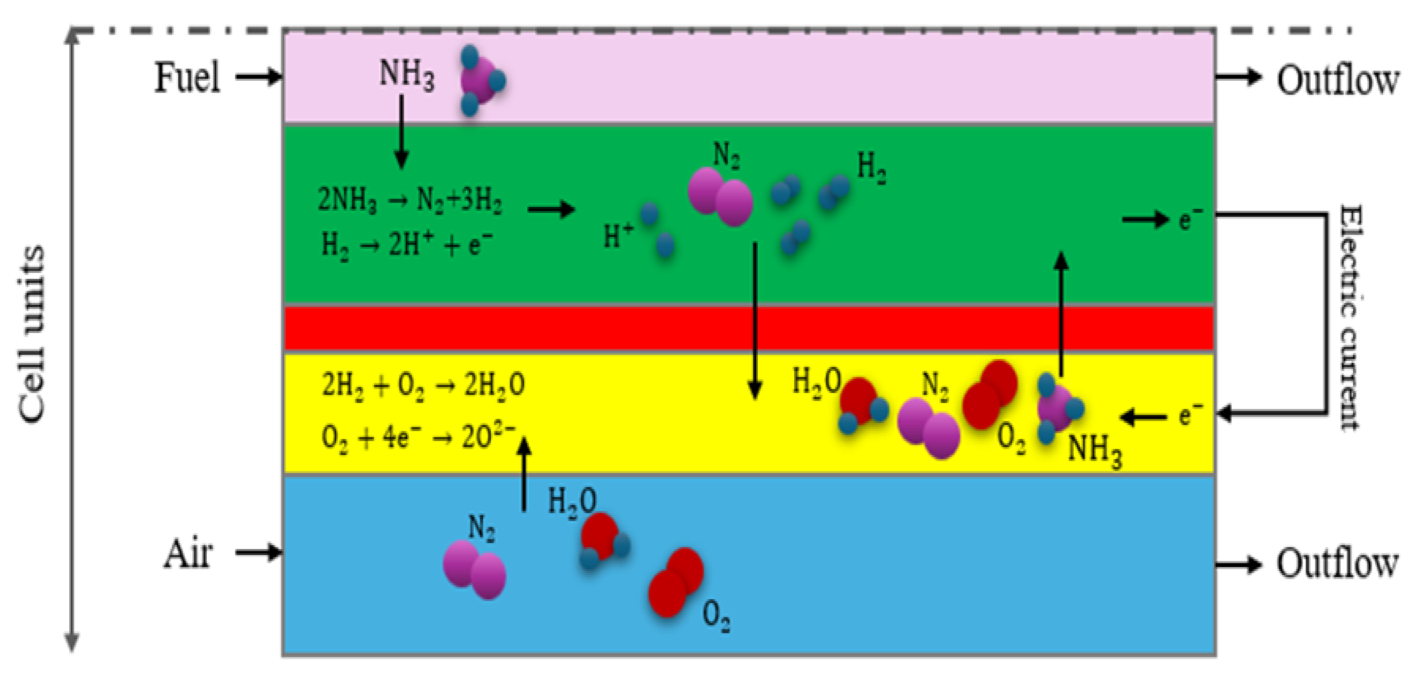
Figure 2.
Validation diagram.
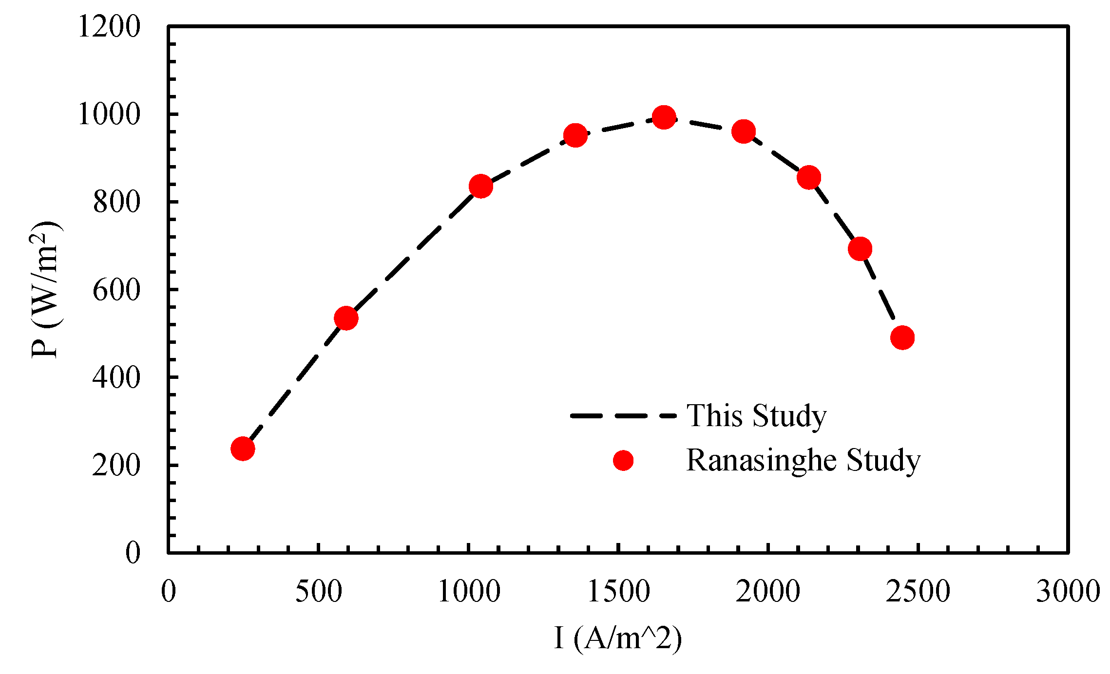
Figure 2.
Pearson Correlation Coefficient.
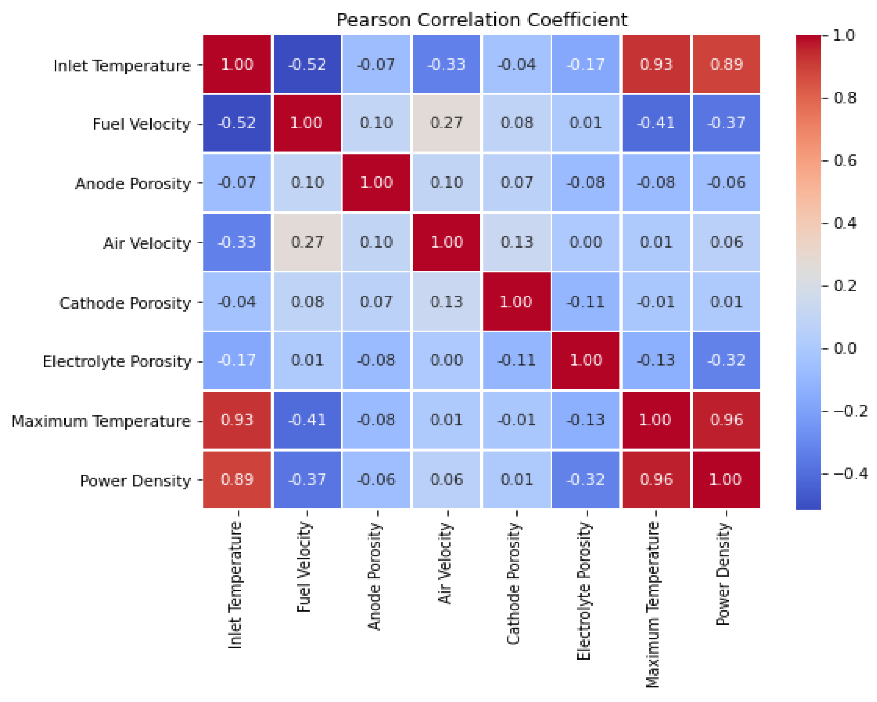
Figure 7.
Comparison of XG Boosting and Support Vector Machine in Prediction of Power Density.
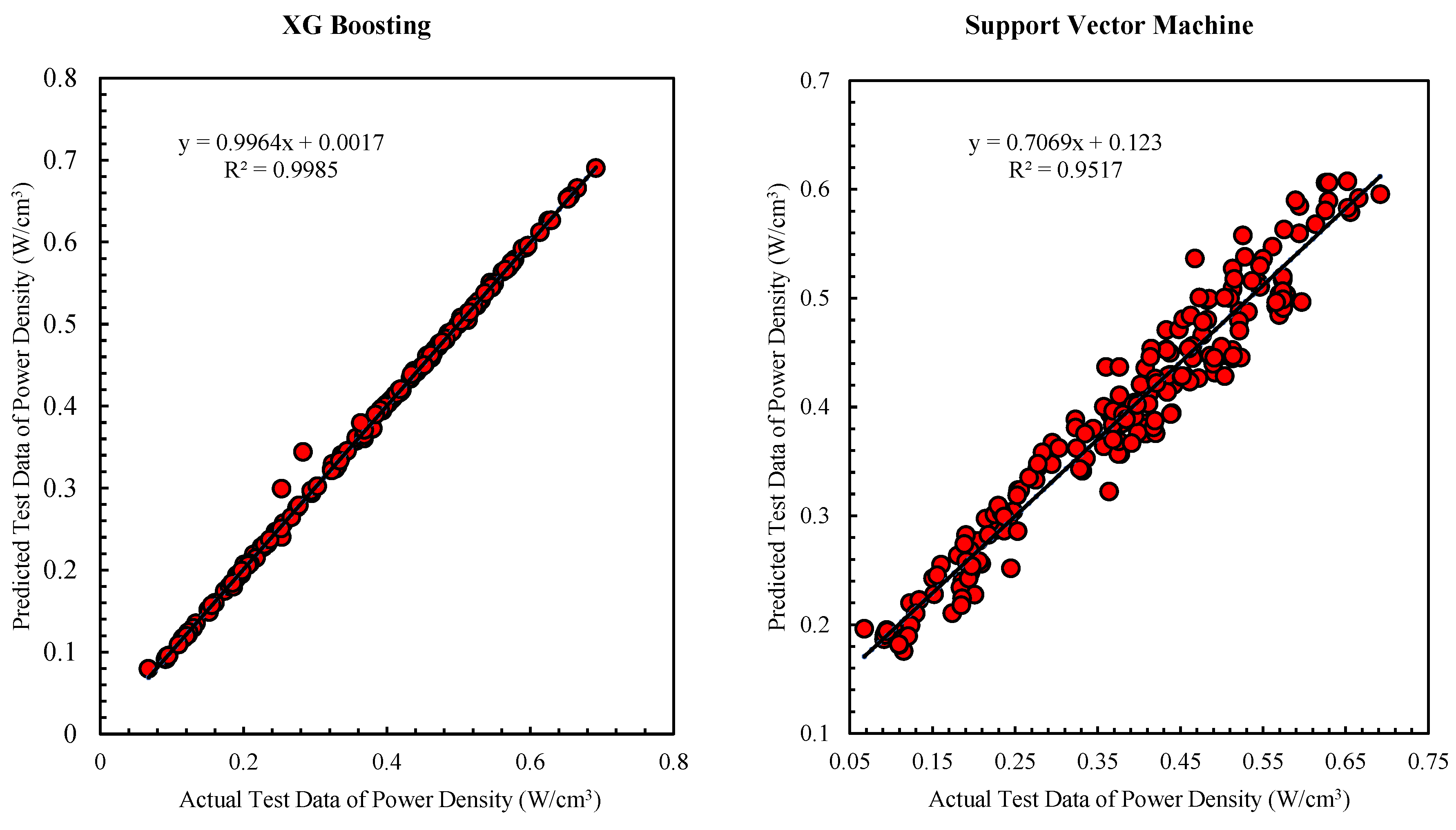
Figure 8.
Comparison of XG Boosting and K Neighbours in Prediction of Power Density.
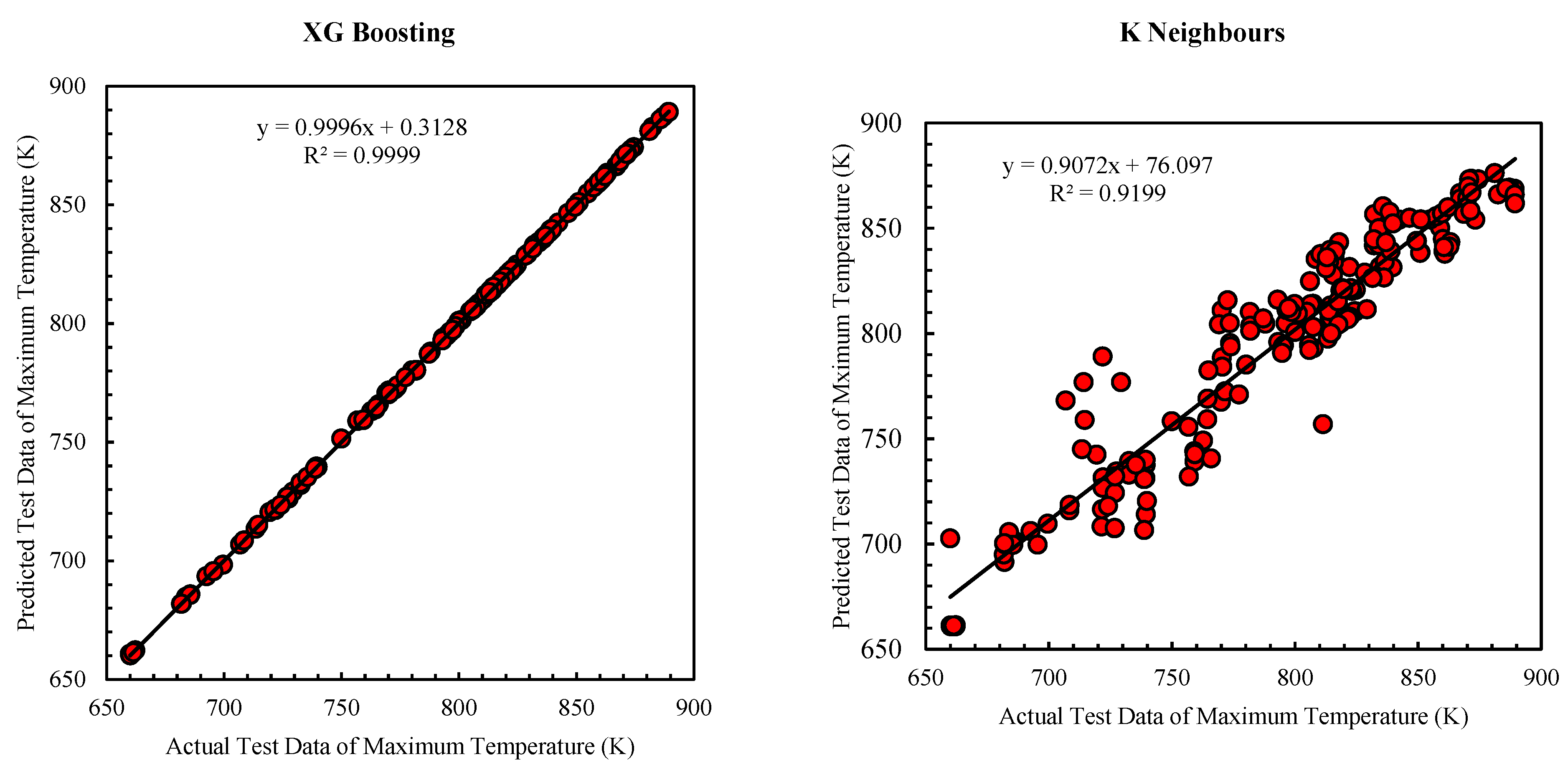

Table 1.
Size of the various parts of the fuel cell.
| Parameter | Size (mm) |
|---|---|
| Fuel channel radius | 0.35/2 |
| Anode thickness | 0.35 |
| Electrolyte thickness | 0.01 |
| Cathode thickness | 0.06 |
| Air channel thickness | 0.35 |
| Fuel cell length | 10 |
Table 2.
Statistical Data Status.
| Parameters | Inlet Temperature |
Fuel Velocity | Anode Porosity | Air Velocity |
Cathode Porosity | Electrolyte Porosity |
Maximum Temperature | Power Density | |
|---|---|---|---|---|---|---|---|---|---|
| Count | 1030.00 | 1030.00 | 1030.00 | 1030.00 | 1030.00 | 1030.00 | 1030.00 | 1030.00 | |
| Mean | 862.63 | 0.26 | 0.32 | 0.28 | 0.34 | 0.11 | 789.08 | 0.37 | |
| STD | 92.94 | 0.09 | 0.06 | 0.10 | 0.06 | 0.10 | 62.34 | 0.16 | |
| Min | 673.00 | 0.10 | 0.10 | 0.10 | 0.10 | 0.0001 | 654.64 | 0.07 | |
| 25% | 800.00 | 0.15 | 0.25 | 0.20 | 0.30 | 0.01 | 739.56 | 0.23 | |
| 50% | 900.00 | 0.25 | 0.35 | 0.30 | 0.35 | 0.10 | 805.44 | 0.41 | |
| 75% | 950.00 | 0.35 | 0.35 | 0.35 | 0.40 | 0.20 | 836.47 | 0.49 | |
| Max | 973.00 | 0.50 | 0.50 | 0.50 | 0.50 | 0.50 | 890.70 | 0.69 |
Table 3.
Machine Performance in Power Density Prediction with Various algorithms.
| Regression Models | RMSE_train | MAE_train | R2_Train | RMSE_test | MAE_test | R2_test |
|---|---|---|---|---|---|---|
| Linear | 0.03099652 | 0.02289843 | 0.96183529 | 0.03154692 | 0.02413547 | 0.95963308 |
| Stochastic Gradient Descent | 0.03101462 | 0.02277184 | 0.96179071 | 0.03167708 | 0.02407398 | 0.95929927 |
| Ridge | 0.03099653 | 0.02289313 | 0.96183526 | 0.03154936 | 0.02413246 | 0.95962682 |
| Decision Tree | 0.00000000 | 0.00000000 | 1.00000000 | 0.01102635 | 0.00309556 | 0.99506854 |
| Random Forest | 0.00193758 | 0.00101979 | 0.99985087 | 0.00892497 | 0.00380967 | 0.99676909 |
| Support Vector Machine | 0.05483591 | 0.04573663 | 0.88055549 | 0.05402141 | 0.04557084 | 0.88162947 |
| Lasso | 0.03113737 | 0.02255870 | 0.96148766 | 0.03170878 | 0.02377720 | 0.95921778 |
| Gradient Boosting | 0.00630288 | 0.00459090 | 0.99842197 | 0.00727113 | 0.00528423 | 0.99785555 |
| K Neighbors | 0.03218481 | 0.02503208 | 0.95885302 | 0.04547824 | 0.03457744 | 0.91610828 |
| XG Boosting | 0.00136861 | 0.00102359 | 0.99992560 | 0.00613662 | 0.00249331 | 0.99847254 |
| Artificial Neural Network | 0.03099678 | 0.02286982 | 0.96183465 | 0.03155168 | 0.02410902 | 0.95962090 |
Table 4.
Machine Performance in Maximum Temperature Prediction with Various algorithms
| Regression Models | RMSE_train | MAE_train | R2_train | RMSE_test | MAE_test | R2_test |
|---|---|---|---|---|---|---|
| Linear | 9.634103 | 7.533192 | 0.976046 | 10.47626 | 7.887151 | 0.971602 |
| Stochastic Gradient Descent | 9.635198 | 7.519635 | 0.97604 | 10.46618 | 7.862889 | 0.971657 |
| Ridge | 9.634109 | 7.534488 | 0.976045 | 10.47671 | 7.888727 | 0.9716 |
| Decision Tree | 0 | 0 | 1 | 1.005492 | 0.341553 | 0.999738 |
| Random Forest | 0.388605 | 0.188909 | 0.999961 | 1.193282 | 0.461912 | 0.999632 |
| Support Vector Machine | 0.896029 | 0.498045 | 0.999793 | 1.238221 | 0.791369 | 0.999603 |
| Lasso | 9.634103 | 7.533444 | 0.976046 | 10.47658 | 7.887702 | 0.9716 |
| Gradient Boosting | 1.765142 | 1.162257 | 0.999196 | 2.037377 | 1.388921 | 0.998926 |
| K Neighbors | 12.70697 | 9.762762 | 0.958328 | 14.25822 | 10.52725 | 0.947398 |
| XG Boosting | 0.088429 | 0.059149 | 0.999998 | 0.518606 | 0.23728 | 0.99993 |
| Artificial Neural Network | 9.634103 | 7.533192 | 0.976046 | 10.47626 | 7.887151 | 0.971602 |
Disclaimer/Publisher’s Note: The statements, opinions and data contained in all publications are solely those of the individual author(s) and contributor(s) and not of MDPI and/or the editor(s). MDPI and/or the editor(s) disclaim responsibility for any injury to people or property resulting from any ideas, methods, instructions or products referred to in the content. |
© 2025 by the authors. Licensee MDPI, Basel, Switzerland. This article is an open access article distributed under the terms and conditions of the Creative Commons Attribution (CC BY) license (http://creativecommons.org/licenses/by/4.0/).
Copyright: This open access article is published under a Creative Commons CC BY 4.0 license, which permit the free download, distribution, and reuse, provided that the author and preprint are cited in any reuse.


