A Gis-Based Decision Support Model (DSM) for Harvesting System Selection on Steep Terrain: Integrating Operational and Silvicultural Criteria

1. Introduction

Logging operations on steep terrain present significantly greater challenges compared to those conducted on gentle slopes, due to increased risks of environmental damage, higher operational costs, greater technical complexities, and more severe worker safety issues (Jordan et al., 2010; Visser & Stampfer, 2015). As a result, it becomes critical to carefully select the most appropriate harvesting system for such conditions. In that regard, operators face two main alternatives: ground-based machine systems and cable-based machine systems.

Ground-based machine systems (GBS) are generally associated with higher productivity levels due to their efficiency in accessing and processing timber (Spinelli et al., 2016). However, cable-based machine systems (CBS) result in significantly less stand damage, which makes them preferable in ecologically sensitive areas (Holzfeind et al., 2020; Schweier & Ludowicy, 2020). The challenge lies in identifying the optimal system for each particular site, one that achieves a balance between high productivity and low environmental impact.

That decision can be guided by five key criteria: slope gradient, soil bearing capacity, geomorphological hindrances (the ground obstacles such as rocks or debris), the existing forest road network, and sensitive zones that are restricted from timber harvesting, including stream management zones (SMZ), biotopes and other special protection areas. Those criteria collectively influence the feasibility, safety, and environmental impact of the chosen harvesting system (Piragnolo et al., 2019). A thorough understanding and accurate assessment of those factors are paramount to successful planning.

To optimize information acquisition and analysis for those criteria, Geographic Information System (GIS)-based approaches are invaluable. GIS provides a powerful platform for integrating spatial data, enabling precise mapping, modeling, and decision-making. By employing GIS tools, forest managers can develop tailored, site-specific harvesting plans that not only maximize productivity but also ensure sustainability and compliance with environmental protection standards (Sivrikaya et al., 2010).

This study aims at developing a systematic procedure for selecting the most appropriate harvesting system for each specific forest area, based on remotely sensed site and stand characteristics. The proposed method comprehensively incorporates all the above listed criteria essential for determining whether a forest is suitable for harvesting and, if so, which harvesting system should be applied. Furthermore, an additional factor, which ideally plays a critical role in optimizing the selection of harvesting machine configurations, is considered. This factor, distinct from site conditions, pertains to the forest stand characteristics—specifically, the silvicultural criterion. Within this context, the silvicultural criterion is primarily represented by the distribution of stem diameters across various patches of the forest stand.Therefore, stem diameter classes are used to integrate silvicultural objectives into operational planning, and not just to guide machine selection based on its capability to handle certain tree sizes (Mederski et al., 2019; Spinelli & Magagnotti, 2010). Mapping the spatial distribution of diameter classes within the stand is rather meant to help forest managers in implementing silvicultural considerations alongside technical constraints within operational planning.

This combined information enables the forest manager to strategically plan operational corridors, aligning harvesting activities with silvicultural goals such as selective thinning, regeneration promotion, or habitat preservation. Such a map provides a practical tool for harmonizing technical feasibility with ecological and management objectives, making the planning process both efficient and silviculturally effective.

Jodłowski and Kalinowski (2018) examined the technical and economic feasibility of mechanized harvesting systems in mountainous areas, using literature reviews, case studies, and GIS data, though silvicultural aspects were not integrated. Cavalli and Amishev (2019) evaluated winch-assisted harvesting on steep terrain but did not provide practical decision tools. Klosterhuber and Plettenbacher (2013) analyzed harvesting systems in South Tyrol, focusing on road networks, slope gradients, geomorphology, and cost-efficiency. They identified ecological considerations but lacked forest stand integration. Phelps et al. (2021) developed a GIS-based tool for wheel-based harvesting machinery, considering slope, skidding distance, and stand age as a proxy for timber volume, but it did not enable fine-scale silvicultural recommendations. Bont et al. (2022) created a decision tool incorporating GIS, NFI data, and decision trees to optimize system selection but excluded individual tree-level data. Advanced technologies like ALS and drones have been studied for detailed forest stand analysis (Miraki et al., 2021; Stereńczak et al.; Zhang et al., 2016). Research into deep learning for ecological data processing (Goodwin et al., 2022; Zhao et al., 2023) includes applications for drone-captured data (Diez et al., 2021; Persson, 2024). Studies also explore the DeepForest package for analyzing drone-derived data (Bennett et al., 2022; Gan et al., 2023; Sivanandam & Lucieer, 2022).

Collectively, these studies call for the integration of widely available tools and datasets into a unified, streamlined procedure. Such a framework would utilize (i) orthophotos with three spectral bands for tree detection (instead of drone captured images); (ii) the open-source DeepForest Python module for tree crown identification; (iii) allometric functions to estimate tree diameters based on crown dimensions; (iv) digital terrain models (DTM) and digital surface models (DSM) for site assessments; and (v) GIS tools (QGIS, SAGA GIS, GRASS GIS) for mapping criteria.

For the purpose of this study, field validation was conducted in a Norway spruce-dominated test area in South Tyrol, Italy and consisted of field surveys to validate the accuracy of remote sensing-based predictions against ground measurements. Two main assumptions shaped the study: i) a focus on highly mechanized logging systems and ii) the exclusion of cost, productivity, and efficiency analyses. The novelty of the proposed method lies in its practical and budget-friendly approach, requiring only three initial raster layers, orthophoto, digital terrain model (DTM) and digital surface model (DSM), and the use of an open-source computer vision algorithm, combined with a silvicultural focus to guide harvesting system selection and operational planning.

2. Methods and Materials

For the purpose of this study, the following harvesting systems were considered: (i) a standard harvester-forwarder system (wheeled or tracked), where felling and processing are conducted by the harvester and extraction by the forwarder; (ii) a winch-assisted harvester- forwarder system, where the machines are tethered by a winch for use in steep terrain; and (iii) a tower yarder system, where felling is performed motor-manually with chainsaws, extraction by a tower yarder and processing by a roadside processor (possibly integrated within the tower yarder unit). Both ground-based and cable-based systems encompass two distinct alternatives: a small-scale application, designed to efficiently handle logs with a mean diameter of up to 20 cm, and a large-scale application, tailored to meet the requirements for processing logs with diameters exceeding 20 cm.

GIS technology was used to analyze and map site-specific and stand-specific criteria. Two GIS platforms were employed: QGIS (QGIS Development Team, 2024), which integrates tools from the SAGA GIS environment (Conrad et al., 2016), and GRASS GIS (GRASS Development Team, 2024).

Raster layers were generated for each criterion to allow spatially explicit predictions for every point within the study area. Six criteria were analyzed: five of them being site-specific (layers i) to v) in the following) and one stand-specific (layer vi):

i) The first layer mapped watercourses using data from the official geoportal of the South Tyrolean Citizen Network (Geoportal of South Tyrol, 2024). A buffer of 10 meters on either side of all watercourses was excluded from harvesting activities.

ii) The second layer represented the forest road network. Since soil disturbance and compaction are essentially influenced by the number of passes of the machines ( Marchi et al., 2014, Picchio et al., 2020) we decided for a rather conservative approach and deemed areas within 200 meters off roads suitable for ground-based systems. This range was delineated using the GRASS GIS tool r.grow.distance. Areas beyond this distance were categorized as suitable for cable-based systems. iii) The third layer, slope, was derived from a digital terrain model (DTM) with a resolution of 2.5 × 2.5 meters, also sourced from the South Tyrol Geoportal.

iv) The fourth layer captured terrain ruggedness, a critical factor for ground-based extraction systems, calculated using the Topographic Roughness Index (TRI) within the SAGA GIS environment (Conrad et al., 2015). The TRI measures the variability in elevation around a specific pixel by calculating the standard deviation of elevations for the neighboring pixels. Parameters were adjusted to reduce sensitivity to abrupt elevation changes, using a linear weighing function for the impact of the distance of pixels around a reference pixel, and a 12.5 × 12.5-meter calculation window to ensure a generalized terrain assessment. v) The fifth layer assessed soil bearing capacity as a topographical proxy for factors like precipitation, permeability, vegetation, bedrock, and soil type. As such the Topographical Wetness Index (TWI) was used (GRASS Development Team, 2024): that estimates the potential for soil moisture accumulation in the landscape, and is calculated according to the formula:

$$\mathrm{T}\mathrm{W}\mathrm{I}=\mathrm{l}\mathrm{n} ({\displaystyle \frac{\mathrm{u}\mathrm{p}\mathrm{s}\mathrm{l}\mathrm{o}\mathrm{p}\mathrm{e} \mathrm{c}\mathrm{a}\mathrm{t}\mathrm{c}\mathrm{h}\mathrm{m}\mathrm{e}\mathrm{n}\mathrm{t} \mathrm{a}\mathrm{r}\mathrm{e}\mathrm{a}}{\mathrm{t}\mathrm{a}\mathrm{n} \left(\mathrm{s}\mathrm{l}\mathrm{o}\mathrm{p}\mathrm{e}\right)}})$$

(1)

The Topographic Wetness Index (TWI) intuitively indicates that larger catchment areas combined with gentler slopes are more prone to water accumulation, resulting in higher index values. This insight was essential for evaluating soil bearing capacity in the context of mechanized ground-based harvesting.

vi) The sixth layer incorporated the distribution of diameter at breast height (DBH) classes, which is critical for determining the appropriate harvesting system, as well as assessing silvicultural goals and practice. This layer was generated through a series of computational steps:

Step 1: Tree detection from orthophotos: The tree detection process employed the open-source deep-learning algorithm DeepForest (Weinstein et al., 2020), which is built on Convolutional Neural Networks (CNNs). DeepForest is available as a Python module, making it accessible and easy to integrate into various workflows. This algorithm is specifically designed to detect tree crowns from high-resolution aerial imagery, offering a pre-trained model ready for immediate use while also providing the flexibility to create fine-tuned models tailored to custom datasets. To fine-tune the DeepForest model for the context of this study, the process involved the following steps: First, a test section of the area, represented by the orthophoto, was selected. Predictions were made using the DeepForest pre-trained model. Ground truth annotations for the test section were then created using the web-based tool LabelMe (Russell et al., 2008). Based on these annotations and the test section image, the DeepForest model was fine-tuned by configuring the hyperparameters as follows: The number of epochs (the total passes the algorithm makes through the entire dataset during training) was set to 10, the learning rate (the step size used for updating the model’s parameters or weights during each iteration) was defined as 0.001; and the batch size (the number of samples in a single pass during the model’s training process) was set to 4. Subsequently, predictions were made using the fine-tuned model. Finally, the outcomes of both the pre-trained and fine-tuned models were compared to the ground truth, and their predictive performances were evaluated by calculating the F1 score (Rijsbergen, 1979).

Since the algorithm cannot reasonably differentiate tree species, we assumed a homogeneous Norway spruce stand, the dominant species in the test area. Given that tree detection accuracy deteriorates when the scale of the orthofoto exceeds a certain limit, the orthofoto was divided into sub-tiles and the optimal size was found based on trial-and-error adjustments to maintain precision. We identified tree positions as the centers of crown rectangles outlined by DeepForest, and calculated crown diameters as the average of the rectangle’s sides. Since the output from DeepForest is an unreferenced PNG file, the extracted data were reprojected to the spatial reference system EPSG:25832 (ETRS89, UTM Zone 32N) for integration into the GIS framework.

Step 2: DBH Calculation: Tree diameters were estimated using allometric functions, which are based on relationships between tree parameters that are measurable through remote sensing, and DBH. Three equations were tested: those of Hasenauer (1997), Pretzsch et al. (2002), and Jucker et al. (2017). The Hasenauer and Pretzsch formulas are calibrated for Central European forests and use tree crown dimensions as the sole predictor variable. Hasenauer based his observations on open grown trees. The Pretzsch formula for Norway spruce has the following form:

$$DBH=e^{{\displaystyle \frac{\log \left(CA\right)-(-1.43)}{1.2}}}$$

(2)

where CA is the Crown Area (m²).

The Hasenauer formula for Norway spruce is expressed as follows:

$$DBH=e^{{\displaystyle \frac{\ln \left(CW\right)-(-0.3232)}{0.6441}}}$$

(3)

where CW is the Crown Width (m).

The third formula is a more generalized model, encompassing a wide range of biogeographic regions and biomes worldwide. It applies to temperate and boreal forests, tropical and subtropical forests, as well as savannas. Unlike more regionally calibrated equations, this formula is designed for broad applicability and utilizes two tree-specific parameters as predictors: crown width and tree height. This formula takes the form:

$$DBH=0.557\ast {(h\ast CW)}^{0.809}\ast e^{{\displaystyle \frac{{0.056}^2}{2}}}$$

(4)

where CW is the crown width (m) and h is the tree height (m).

Step 3: Once the diameters of all trees detected by the computer vision algorithm were obtained, it was necessary to transform the point data into area-related values to evaluate the stocking diameter class for each pixel in the test area. This was achieved using the GRASS GIS v.surf.idw tool, which applies the inverse distance weighting (IDW) algorithm. IDW is an interpolation method that estimates unknown values of the surrounding area based on known point data. Since our tool is designed to support silvicultural decision-making, we focused on leveraging the IDW algorithm to effectively delineate the diverse range of patches within our forest. Therefore, the settings were optimized to perform the interpolation with small areas, ensuring precise representation of spatial variability. Afterwards, the interpolated diameter values were reclassified into homogeneous patches. A threshold of 10 cm was assumed, as silvicultural treatments such as precommercial thinning typically target trees exceeding this diameter (Gauthier & Tremblay, 2018; Simard et al., 2004). Based on this threshold, the following diameter classes were defined: 11–20 cm (pole stage wood), 21–50 cm (tree wood), and >50 cm (old growth).

In addition to the diameters, the tree heights for each tree detected by the computer vision algorithm, was calculated. This was done by creating a Canopy Height Model (CHM), calculated as the difference between the Digital Surface Model (DSM) and the Digital Terrain Model (DTM). Using QGIS’s Sample raster values tool, tree heights were extracted at the precise tree-top coordinates.

Finally, all the generated layers were superimposed to evaluate the optimal harvesting configuration for each pixel of the test area. This spatial analysis was conducted using the GRASS GIS r.mapcalc function. Compared to other similar tools such as the QGIS raster calculator, r.mapcalc offers the advantage of handling complex mathematical operations across multiple layers, making it particularly suited for the multifaceted requirements of this study. This functionality allowed seamless integration of diverse criteria, enabling a pixel-by-pixel assessment of the most suitable harvesting configuration across the test area.

To execute the generated model, predefined thresholds for specific harvesting systems were applied to account for terrain and operational constraints. For example, ground-based logging systems were limited by maximum allowable slopes, TRI (Terrain Ruggedness Index), and TWI (Topographic Wetness Index) values. The key assumptions were as follows: standard harvester/forwarder systems were deemed suitable for slopes of up to a 40% incline, while winch-assisted harvester/forwarder systems could operate effectively on slopes up to 100%. For slopes exceeding the 100% incline, cable-based systems were identified as the only viable option (Leslie, 2019; Marchi et al., 2018; Obi & Visser, 2020). For low-impact operations using ground-based machines, maintaining a Topographic Ruggedness Index (TRI) not larger than 1 and a Topographic Wetness Index (TWI) not larger than 5 is critical to minimizing environmental disturbance. If operations can tolerate greater environmental impacts, the allowable thresholds increase, with TRI capped at a maximum of 2 and TWI not exceeding 10 (Pourali et al., 2016).

Validation of results was crucial to this study and was achieved by applying the model to a test area and then performing on-site field measurements for validation of stand measurement predictions. A systematic grid was created using the Polygon Divider and Centroids tools in QGIS, resulting in 30 fixed sample plots. Each plot had a diameter of 15.96 m, covering an area of 200 m². Within these plots, the following parameters were recorded: tree species, diameter at breast height (DBH) of each tree, and the height of the mean tree.

The primary goal of comparing field data with the DeepForest algorithm’s outputs was to assess whether the algorithm failed to detect certain trees and, if so, to determine the proportion of undetected trees. An additional objective was to evaluate whether the algorithm exhibited biases in detecting trees across diameter classes. Specifically, the analysis sought to identify whether the algorithm disproportionately overlooked trees in the pole-stage wood class compared to the other two growth classes (tree wood and old growth) or vice versa, while excluding trees below a 10 cm diameter. Furthermore, terrain validation aimed at selecting the most accurate of the three formulas used for estimating diameter at breast height (DBH) from crown size. To that end, we employed the two-sample Anderson-Darling test (Anderson & Darling, 1952), which is sensitive to differences in the tails of data distributions. In addition, the following accuracy metrics were adopted: the mean absolute error (MAE) i.e. the average of the absolute differences between predicted and observed values, the mean bias error (MBE) i.e. the average of the differences between predictions and observations, and the normalized root mean square error (NRMSE) which is the mean square error of the differences, normalized by the range of the observations. Each formula underwent rigorous testing, and the one providing the closest alignment with the empirical data was ultimately adopted.

Test Area

Our 91.2-hectare test area is situated in the municipality of Rasen-Antholz/Rasun-Anterselva in South Tyrol, Italy. This steep, north-facing slope has an average inclination of 48% and is characterized by two notable features. First, it exhibits a fragmented ownership structure, leading to inconsistent forest management practices across the various wood lots. Second, the area has experienced increasing bark beetle infestations in recent years, prompting salvage logging through clear-cutting on many affected patches. Those dynamics have contributed to a highly uneven-aged forest structure, reflecting the combined influence of small-scale management practices and disturbance-driven regeneration patterns. All analyses were performed using Python (version 3.11.7) [Python Software Foundation, 2023].

3. Results

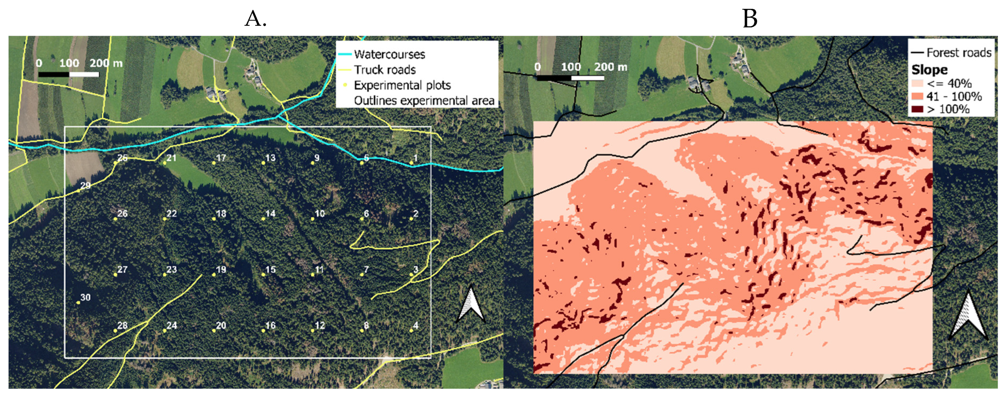
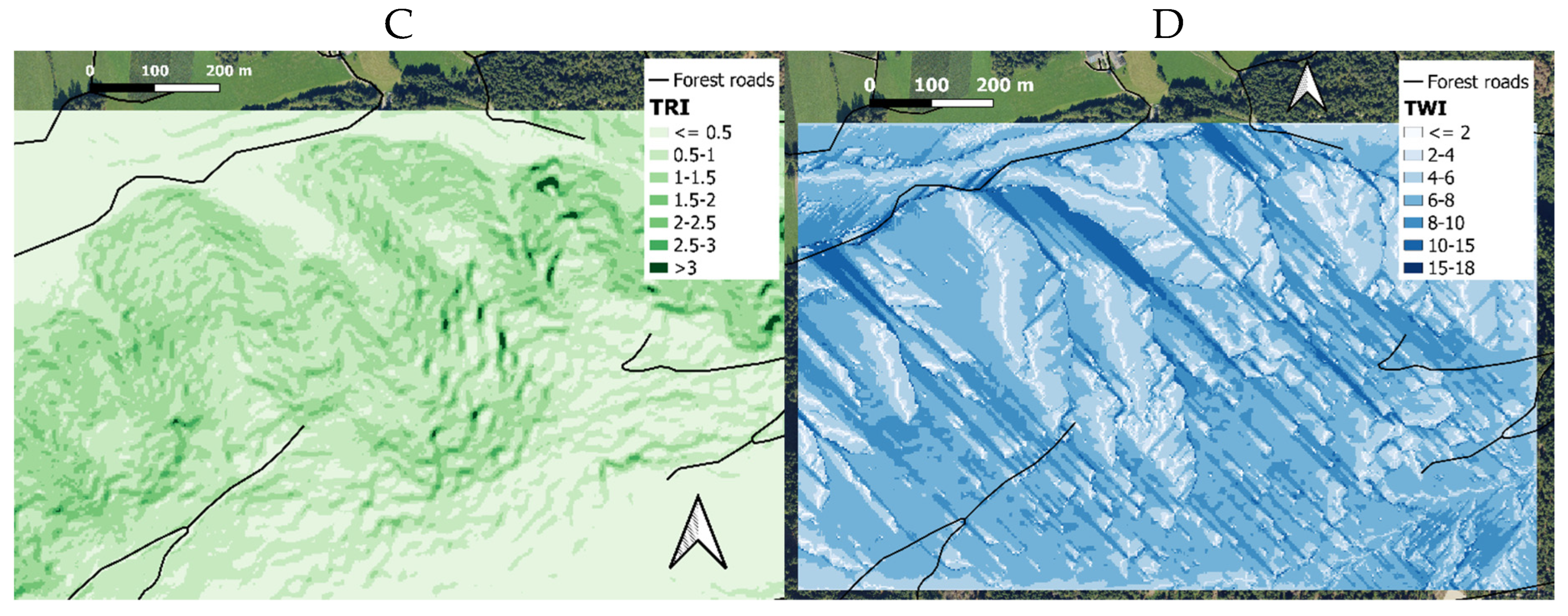
In the following section, we present the raster layers derived using the methodology described above. Each raster layer represents one of the six criteria analyzed to identify the most suitable harvesting system. Figure 1A illustrates the experimental area, showing the plot locations established for on-site validation of the results. The figure also displays the forest road network and the watercourses within the experimental site. Notably, the spatial decision-support model incorporated these two layers, with forest roads and watercourses represented in rasterized form. Figure 1B depicts the slope map, where values were grouped into three functional classes for clarity: up to 40%, between 40% and 100%, and above 100%. Figure 1C shows the layer for the Topographical Ruggedness Index (TRI), used as a proxy for terrain undulation. The values for TRI on our test area range from 0.006 to 4.237. Figure 1D presents the mapping of the Topographical Wetness Index (TWI): higher values are observed in ditches where the terrain is concave, and lower values on ridges where the terrain is convex. This alignment becomes particularly evident when comparing the TWI layer with the orthophoto in Figure 1A, demonstrating the reliability and spatial accuracy of the results. The values for TRI on our test area range from 0.0 to 18.841.

The generation of the sixth layer for the spatial decision support model involved three distinct work steps: tree crown identificationestimate of tree diameter, and stem diameter class mapping.

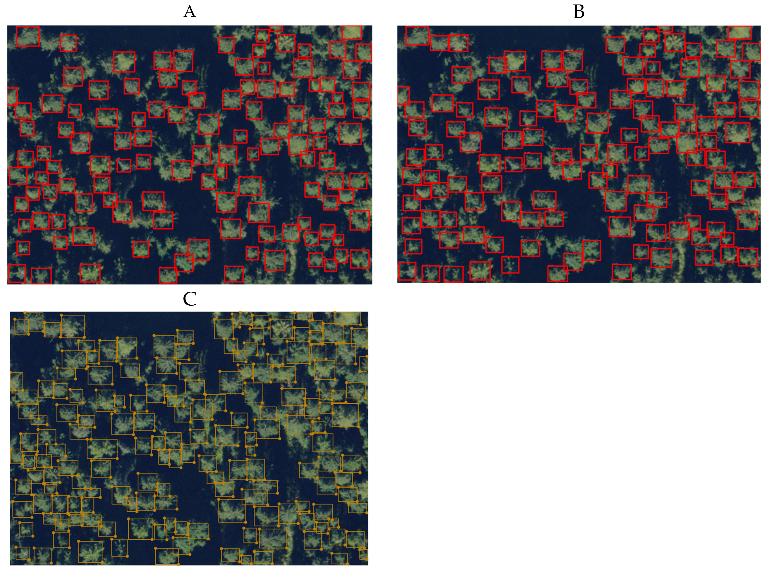
The result of step one is illustrated in Figure 2. It provides the test section for the fine-tuning of the DeepForest algorithm. The tree crowns identified by using the pre-trained model before and after fine-tuning are shown in Figure 2A,B, respectively Finally, the ground truth as delineated by hand is shown in Figure 2C.

The predictive performance of the two models was assessed using the following paarmeters: Precision, Recall and F1 score (Table 1).

The share of overlooked trees for both models (i.e. pre-trained and fine-tuned) is around 30%. Precision is notably higher than Recall, highlighting that the algorithm makes fewer errors in identifying trees where none exist (False Positives) than it fails to identify actual trees (False Negatives, i.e., overlooked trees). The F1 represents the harmonic mean of Precision and Recall. The fine-tuned model (F1 = 0.794) performs slightly better than the pre-trained model (F1 = 0.752). Therefore, the former was adopted for the purpose of this study.

Regarding the field measurements, data collection was successfully conducted on 28 out of the intended 30 sample plots. One of the plots fell within an agricultural field (see Figure 1A), rendering it unsuitable for the study, while another plot was inaccessible due to the extreme steepness of the terrain.

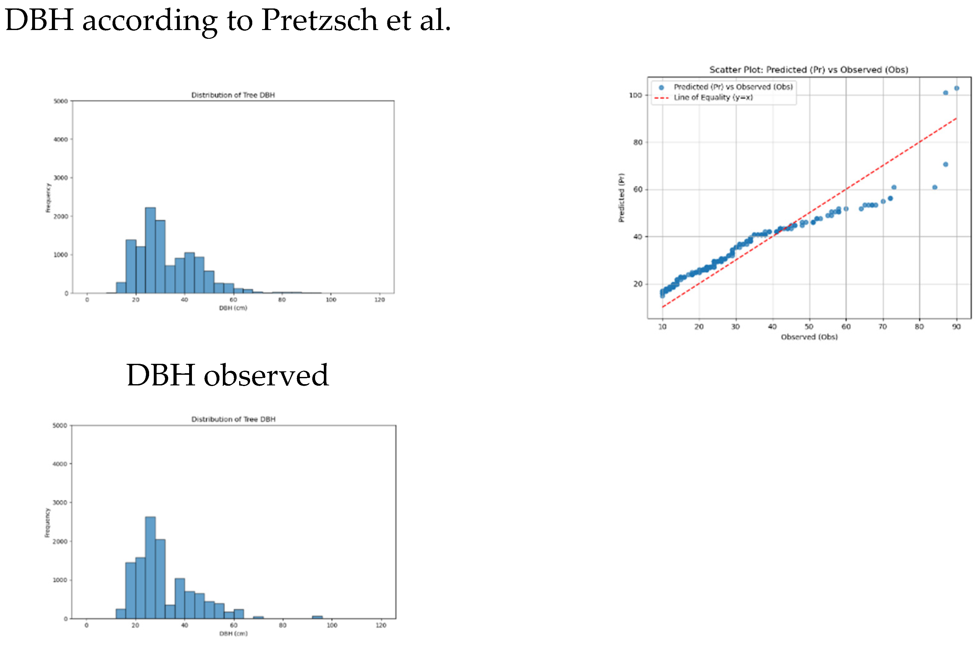
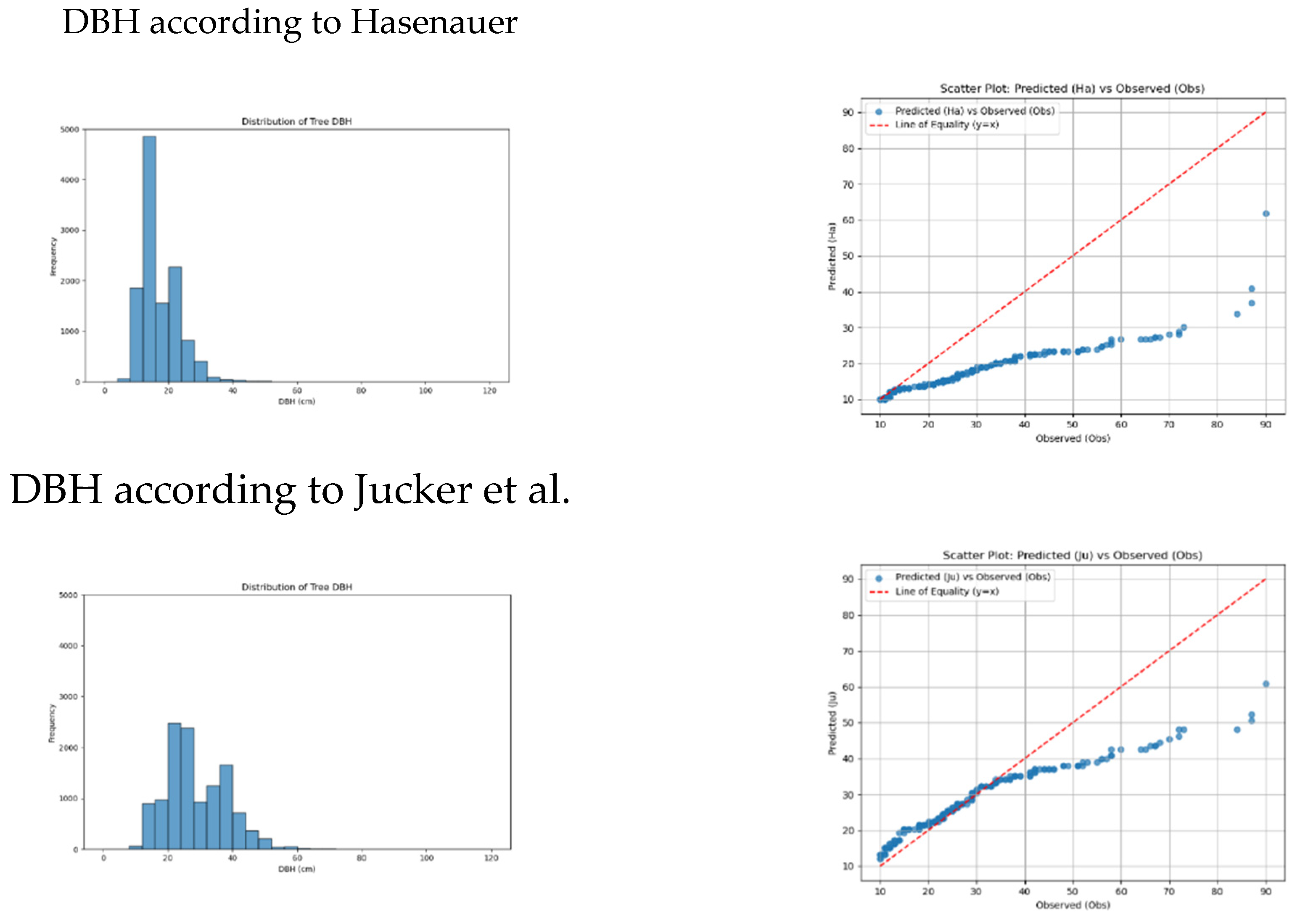
The outcome of work step two (comparison of the calculated vs. actual DBH values) is presented in Figure 3 and Table 2. Figure 3 shows the data distribution of the theoretically derived values for tree DBH, and matches that distribution with the actual one, as determined through field measurements (Figure 3 left hand). Additionally, Figure 3 contains the scatterplots when plotting the differences of predicted minus observed values (Figure 3 right hand).

The following Table 2 provides a comprehensive summary of descriptive statistics for DBH and height values, including the distribution of frequencies across DBH classes. Additionally, it details the calculated metrics comparing the predicted DBH values against the observed DBH, offering insights into the accuracy and performance of the predictive models.

On average, the Deepforest algorithm identified 147 trees per hectare, compared to the actual stem count of 350 trees (above a threshold diameter of 10 cm), thus underestimating tree count by 138%.

The two-sample Anderson-Darling test indicates that none of the DBH predictions align with the observed data distributions. Predictions using Hasenauer’s method significantly overestimate the abundance of smaller trees (DBH 10–20) while markedly underestimating larger trees (DBH >50). In contrast, predictions based on the Jucker formula consistently underestimate the size of larger trees. Similarly, estimates derived from Pretzsch’s formula tend to underestimate both smaller and larger trees, albeit to a lesser degree than the other methods. Among the models, the Pretzsch formula achieves the highest accuracy metrics (MAE, MBE, NRMSE) for DBH predictions, demonstrating comparatively better alignment with the observed values.

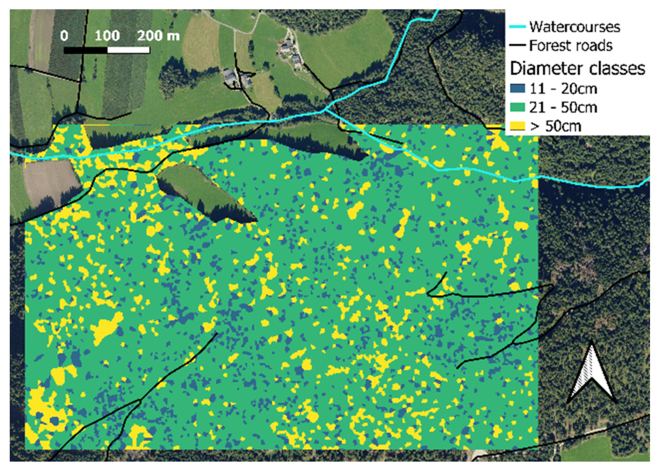
Results for the third step are shown in Figure 4, which presents the location of diameter classes within the experimental area, determined using the GRASS GIS tool v.surf.idw. This tool interpolates DBH point data to generate area-related diameter distribution information.

Figure 4 represents the spatial variation in tree diameters across the study site, enabling a detailed understanding of the diameter class distribution derived from the interpolation process. According to this analysis, the diameter class 11-20cm covers 11%, the diameter class 21-50cm 74%, and the diameter class >50cm 15% of the forested area. These figures deviate slightly from the stem number percentages (14%, 76%, 10%; see Table 2) due to the disproportionate spatial contribution of trees of different sizes. Specifically, a larger number of small trees is required to occupy the same area that can be covered by a comparatively smaller number of large trees.

The six key layers that inform the harevsting system selection model are processed using the GRASS GIS tool r.mapcalc, which employs conditional if-statements to implement the predefined capability assumptions for the three technology alternatives (i.e. standard harvesters-forwarders, tethered harvester-forwarder and cable yarder).

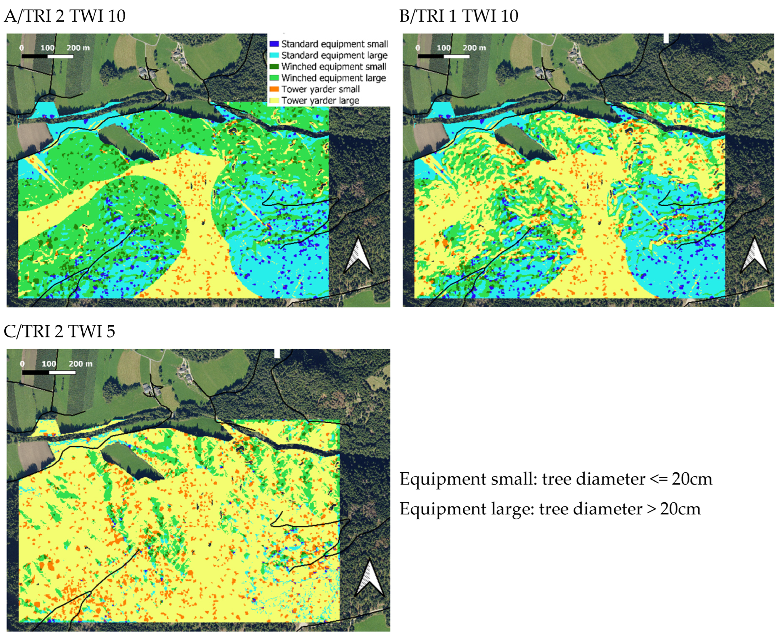
For illustration purposes, we conducted three test runs of the generated model, varying the values for the TRI and TWI layers to explore different management preferences. In the first run, we assumed forest managers to prioritize ground-based equipment and to exhibit less concern for environmental impacts, thus permitting machine operation up to a TRI of 2 and a TWI of 10. The results of this scenario are depicted in Figure 5A. In the second and third runs, we postulate forest managers to adopt a more restrictive approach, emphasizing reduced environmental impact. For the second test (Figure 5B), we hypothesize a maximum allowable TRI of 1 and a TWI of 10. In the third run (Figure 5C), we limit the parameters to a TRI of 2 and a TWI of 5.

Table 3 displays the percentages of the area allocated to the three different harevsting systems, for those three scenarios.

Ground-based equipment operates exclusively within the defined 200-meter proximity to forest roads and beyond the 10-meter buffer zone on either side of existing watercourses (Figure 5). Additionally, areas with slopes exceeding 150% remain unharvested, as indicated by the spots displaying the bare orthophoto colors. When setting the TRI to 2 and the TWI to 10, the zone inside the 200m distance to forest roads can almost entirely be operated by ground-based equipment (Figure 5A; ). When considering the total test area, in this scenario the percentage for ground-based logging is 71%, and for cable-based logging 19% (Table 3). When the TRI value is reduced from 2 to 1 (Figure 5B), the areas suitable for ground-based machinery decrease to 52% of the total, whereas those suitable for cable- logging increase to 38% (Table 3). Finally, when the TWI value is lowered from 10 to 5 (Figure 5C), ground-based logging drops to 22% of the total area and cable-based logging climbs to 68% (Table 3). That highlights the substantial impact of TWI (soil bearing capacity) on the applicability of ground-based logging.

4. Discussion and Conclusion

To ensure a balanced perspective, we first outline the limitations of the presented decision support model before delving into its strengths, which are discussed further below.

Currently, the DeepForest algorithm, when applied to orthophotos, struggles to accurately distinguish between tree species. Even fine-tuning the algorithm with ground truth data does not fully address this limitation. As a result, our study had to generalize tree species based on the dominant species in each given area.

Another limitation is that the algorithm, when compared to ground-collected data, significantly underestimates the number of trees, missing a substantial portion by a margin of 138% (Table 2). This tendency to overlook trees, particularly in the smaller diameter class, has also been observed by Persson (2024).

However, a more detailed examination of these findings is essential. With certainty, we can only state that the Deepforest algorithm overlooks a certain number of trees, but we cannot say for sure if most of these overlooked trees are in the lower or upper end of the size distribution. This uncertainty persists even if we contrast the predicted numbers with ground-collected data since we cannot directly compare crowns identified by the algorithm with those observed on the ground. Instead, we can only compare diameters calculated from predicted crowns to those measured on the ground. Errors in these predicted diameters could arise from two sources: limitations in the tree detection algorithm or flaws in the allometric function used to estimate diameters.

For example, using Hasenauer’s function, there seems to be no shortage of small trees (Table 2). But when considering the overall distribution of tree diameters, Pretzsch’s function appears to provide the most reliable results. It predicts a balanced distribution of small, medium, and large trees for the test region. Assuming that Pretzsch’s formula is the most accurate one out of the three tested functions, our method predicts significantly fewer small trees (14% versus 29% observed) and fewer large trees (10% versus 14% observed) (Table 2). The underestimation of small trees is likely due to the tree detection algorithm failing to detect them when they are hidden beneath the canopy’s top layer.

Conversely, the underestimation of large trees may also stem from the limitations of the allometric function. This limitation arises because tree growth patterns differ as they age. At a certain age, a tree’s height growth slows down, while its diameter growth can accelerate (Fabris, 2000; Larson, 1986). Additionally, crown expansion is more closely related to height growth (Begović et al., 2023) than to diameter growth since trees grow taller primarily to expand their crowns. Once crown growth stabilizes, diameter growth continues, leading to underestimation by functions that calculate diameter based on crown size (Hein & Spiecker, 2009).

As a combination of Deepforest and Pretzsch’s formula, our methodology underestimates the number of small trees, marginally underestimates the number of large trees, and slightly underestimates the size of large trees (Figure 3, Table 2). This indicates a slight bias in the estimations across the diameter classes. However, when looking at the overall performance of the model, the results are more promising. The mean absolute error (MAE) is 5.5 cm, and the average percentage deviation relative to the total diameter range is 6.9% (Table 2), which demonstrates reasonable accuracy for practical applications.

The accuracy of predictions made by algorithms such as DeepForest is subject to a certain degree of variability, which arises from multiple factors, including: the type of forest being analyzed; its density; species diversity; and structural complexity (Hastings et al., 2020). Among these, one of the most critical factors is the quality of the input dataset. High-quality, up-to-date datasets are essential for the algorithm to produce reliable and actionable outputs. It is reasonable to anticipate that the performance of such algorithms will continue to improve over time, driven by advancements in technology and data acquisition methods. In our study, for instance, we observed a significant increase in prediction accuracy when we used the orthophotos from 2023 compared to those from 2020. This improvement underscores the importance of leveraging the latest available datasets, as newer imaging technologies and higher-resolution data can better capture the subtle variations in forest structure, ultimately enhancing the algorithm’s output.

A further limitation of our method is the large amount of work required for setting up the decision support model, which is quite demanding in terms of time and expertise with various software tools. Therefore, the methodology presented here is best considered as a prototype, which will require substantial refinement and automation to make it accessible, seamless, and user-friendly for broader application. Simplifying and streamlining the process will be essential for its adoption by practitioners without advanced technical skills.

Despite the before listed limitations, our decision support model demonstrates functionality and effectiveness. It provides valuable insights into the fundamental characteristics of our experimental forest, offering a clear and practical overview of its current condition and growth patterns. Based on the analyses conducted in this study, forest managers can observe that the experimental forest is predominantly composed of trees in the diameter class ranging from 21 cm to 50 cm, which accounts for 74% of the area. This is followed by the diameter class exceeding 50 cm, representing 15% of the forest area, and lastly, the diameter class from 11 cm to 20 cm, which makes up 11% (Figure 4). From a developmental perspective (Franklin et al. 2002), this distribution indicates that the forest predominantly exists in the maturation stage, characterized by the steady growth of trees and the accumulation of biomass. Smaller portions of the forest represent earlier developmental stages, characterized by biomass accumulation and competitive exclusion (11 cm to 20 cm diameter class), as well as the old growth stage (> 50 cm diameter class) showing advanced structural diversification driven by gap dynamics. These findings provide critical insights into the forest’s current structural composition and offer a baseline for decisions regarding its management, which might include a potential restructuring, whether for economic optimization, ecological sustainability, or a balance of both. Please note that a diameter threshold of 10 cm was applied, so that our study does not give any insights into the dynamics of the early stage of stand development.

Additionally, the spatial maps generated as part of this model allow the forest manager to identify the precise locations of patches corresponding to different growth classes (Figure 4). This spatially explicit information enables the manager to evaluate the suitability of available machinery for specific patches (Figure 5, Table 3). By overlaying the growth class data with operational constraints and available resources (e.g., harvesting machinery available within the company or region), those maps can facilitate informed silvicultural planning. For instance, the manager can decide whether the operational logistics align with the forest’s needs or whether adaptations in the management strategy or machinery might be necessary. As such, the spatial decision support model not only provides a snapshot of the forest’s current state, but also serves as a dynamic tool for future management considerations, promoting efficiency and sustainability in forest operations.

An advancement of the methodology presented here could lead to a single coherent algorithm that integrates all described steps into a streamlined process. This would include assessing operational criteria (based on remotely sensed and publicly available data) such as slope gradient, terrain ruggedness, soil bearing capacity, water bodies, and forest road networks, alongside providing stand data and silvicultural criteria. Specifically, the process would involve tree crown detection via a deep-learning algorithm applied to orthophotos, estimating tree diameters using allometric functions, classifying areas into diameter classes based on those estimates, and finally overlaying all criteria to identify suitable areas for specific harvesting systems. That software should allow users to interactively adjust settings, enabling them to define parameters like diameter class thresholds, maximum machine-operable slopes, critical ruggedness values (TRI), and adjustments for soil bearing capacity (TWI). This flexibility would accommodate varying priorities, such as balancing low-impact measures with economic optimization.

To implement such a system, two approaches are conceivable. The first involves creating additional layers in public geoportals, offering pre-calculated maps that integrate all discussed criteria. For a given region, multiple layers could be made available, each representing different configurations of harvesting systems based on pre-set values for slope, ruggedness, and soil resistance thresholds. The second option is a mobile application (App) that users can download on their cell-phones. This would offer greater interactivity, allowing users to customize settings directly within the app. This approach would provide a much more tailored and dynamic experience compared to the static pre-calculated maps of the geoportal-type solution.

References

- Anderson, T. W., & Darling, D. A. (1952). Asymptotic theory of certain” goodness of fit” criteria based on stochastic processes. The Annals of Mathematical Statistics, 193–212.
- Begović, K., Schurman, J. S., Svitok, M., Pavlin, J., Langbehn, T., Svobodová, K., Mikoláš, M., Janda, P., Synek, M., Marchand, W., & others. (2023). Large old trees increase growth under shifting climatic constraints: Aligning tree longevity and individual growth dynamics in primary mountain spruce forests. Global Change Biology, 29(1), 143–164.
- Bennett, L., Wilson, B., Selland, S., Qian, L., Wood, M., Zhao, H., & Boisvert, J. (2022). Image to attribute model for trees (ITAM-T): individual tree detection and classification in Alberta boreal forest for wildland fire fuel characterization. International Journal of Remote Sensing, 43(5), 1848–1880.
- Bont, L. G., Fraefel, M., Frutig, F., Holm, S., Ginzler, C., & Fischer, C. (2022). Improving forest management by implementing best suitable timber harvesting methods. Journal of Environmental Management, 302, 114099.
- Cavalli, R., & Amishev, D. (2019). Steep terrain forest operations--challenges, technology development, current implementation, and future opportunities. International Journal of Forest Engineering, 30(3), 175–181.
- Conrad, O., Bechtel, B., Bock, M., et al. (2015). System for Automated Geoscientific Analyses (SAGA) v. 7.8. Geoscientific Model Development, 8, 1991–2007. [CrossRef]
- Diez, Y., Kentsch, S., Fukuda, M., Caceres, M. L. L., Moritake, K., & Cabezas, M. (2021). Deep learning in forestry using uav-acquired rgb data: A practical review. Remote Sensing, 13(14), 2837.
- Fabris, S. phanne. (2000). Influence of cambial ageing, initial spacing, stem taper and growth rate on the wood quality of three coastal conifers. University of British Columbia.
- Franklin, J. F., Spies, T. A., Van Pelt, R., Carey, A. B., Thornburgh, D. A., Berg, D. R., Lindenmayer, D. B., Harmon, M. E., Keeton, W. S., Shaw, D. C., & others. (2002). Disturbances and structural development of natural forest ecosystems with silvicultural implications, using Douglas-fir forests as an example. Forest Ecology and Management, 155(1–3), 399–423.
- Gan, Y., Wang, Q., & Iio, A. (2023). Tree crown detection and delineation in a temperate deciduous forest from UAV RGB imagery using deep learning approaches: Effects of spatial resolution and species characteristics. Remote Sensing, 15(3), 778.
- Gauthier, M.-M., & Tremblay, S. (2018). Precommercial thinning as a silvicultural option for treating very dense conifer stands. Scandinavian Journal of Forest Research, 33(5), 446–454.
- Geoportal of South Tyrol (2024). Autonomous Province of Bolzano – South Tyrol. Available online: https://geoportal.buergernetz.bz.it (accessed on 14 September 2024).
- Goodwin, M., Halvorsen, K. T., Jiao, L., Knausgård, K. M., Martin, A. H., Moyano, M., Oomen, R. A., Rasmussen, J. H., Sørdalen, T. K., & Thorbjørnsen, S. H. (2022). Unlocking the potential of deep learning for marine ecology: overview, applications, and outlook. ICES Journal of Marine Science, 79(2), 319–336.
- GRASS Development Team (2024). Geographic Resources Analysis Support System (GRASS GIS) Software (Version 8.4.0). Open Source Geospatial Foundation. Available online: http://grass.osgeo.org.
- Hasenauer, H. (1997b). Dimensional relationships of open-grown trees in Austria. Forest Ecology and Management, 96(3), 197–206.
- Hastings, J. H., Ollinger, S. V, Ouimette, A. P., Sanders-DeMott, R., Palace, M. W., Ducey, M. J., Sullivan, F. B., Basler, D., & Orwig, D. A. (2020). Tree species traits determine the success of LiDAR-based crown mapping in a mixed temperate forest. Remote Sensing, 12(2), 309.
- Hein, S., & Spiecker, H. (2009). 4.3 Controlling Diameter Growth of Common Ash, Sycamore and Wild Cherry. Valuable Broadleaved Forests in Europe, 22, 123.
- Holzfeind, T., Visser, R., Chung, W., Holzleitner, F., & Erber, G. (2020). Development and benefits of winch-assist harvesting. Current Forestry Reports, 6(3), 201–209.
- Jodłowski, K., & Kalinowski, M. (2018). Current possibilities of mechanized logging in mountain areas. Lesne Prace Badawcze, 79(4), 365–375.
- Jordan, P., Millard, T. H., Campbell, D., Schwab, J. W., Wilford, D. J., Nicol, D., & Collins, D. (2010). Forest management effects on hillslope processes. Compendium of Forest Hydrology and Geomorphology in British Columbia. BC Min. For. Range, 66, 275.
- Jucker, T., Caspersen, J., Chave, J., Antin, C., Barbier, N., Bongers, F., Dalponte, M., van Ewijk, K. Y., Forrester, D. I., Haeni, M., & others. (2017). Allometric equations for integrating remote sensing imagery into forest monitoring programmes. Global Change Biology, 23(1), 177–190.
- Klosterhuber, R., & Plettenbacher, T. (2013). Vorrangige Holzernteverfahren auf der technisch nutzbaren Waldfläche in Südtirol und ihre Tauglichkeit für Vollbaumnutzung.
- Larson, B. C. (1986). Development and growth of even-aged stands of Douglas-fir and grand fir. Canadian Journal of Forest Research, 16(2), 367–372.
- Leslie, C. (2019). Productivity and utilisation of winch-assist harvesting systems: case studies in New Zealand and Canada.
- Marchi, E., Picchio, R., Spinelli, R., Verani, S., Venanzi, R., & Certini, G. (2014). Environmental impact assessment of different logging methods in pine forests thinning. Ecological Engineering, 70, 429–436.
- Marchi, L., Grigolato, S., Mologni, O., Scotta, R., Cavalli, R., & Montecchio, L. (2018). State of the art on the use of trees as supports and anchors in forest operations. Forests, 9(8), 467.
- Mederski, P. S., Werk, K., Bembenek, M., Karaszewski, Z., Brunka, M., & Naparty, K. (2019). Harvester efficiency in trunk utilisation and log quality of early thinning pine trees. Forest Research Papers, 80(1), 45–53.
- Miraki, M., Sohrabi, H., Fatehi, P., & Kneubuehler, M. (2021). Individual tree crown delineation from high-resolution UAV images in broadleaf forest. Ecological Informatics, 61, 101207.
- Obi, F., & Visser, R. (2020). Benchmarking 2019 data and longer-term productivity and cost analyses.
- Persson, D. (2024). Tree Crown Detection Using Machine Learning: A study on using the DeepForest deep-learning model for tree crown detection in drone-captured aerial footage. KTH Royal Institute of Technology.
- Phelps, K., Hiesl, P., Hagan, D., & Hotaling Hagan, A. (2021). The harvest operability index (HOI): a Decision support tool for mechanized timber harvesting in mountainous terrain. Forests, 12(10), 1307.
- Picchio, R., Mederski, P. S., & Tavankar, F. (2020). How and how much, do harvesting activities affect forest soil, regeneration and stands? Current Forestry Reports, 6(2), 115–128.
- Piragnolo, M., Grigolato, S., Pirotti, F., & others. (2019). Planning harvesting operations in forest environment: remote sensing for decision support. In ISPRS Annals of Photogrammetry, Remote Sensing and Spatial Information Sciences (Vol. 4, pp. 33–40). Copernicus GmbH.
- Pourali, S. H., Arrowsmith, C., Chrisman, N., Matkan, A. A., & Mitchell, D. (2016). Topography wetness index application in flood-risk-based land use planning. Applied Spatial Analysis and Policy, 9, 39–54.
- Pretzsch, H., Biber, P., & Dursky, J. (2002). The single tree-based stand simulator SILVA: construction, application and evaluation. Forest Ecology and Management, 162(1), 3–21.
- Python Software Foundation. Python Language Reference, version 3.11.7. Available online: https://www.python.org.
- QGIS Development Team. QGIS Geographic Information System. Version 3.32. Open Source Geospatial Foundation Project, 2024. Available online: http://qgis.org.
- Rijsbergen, V. (1979). Information retrieval; Butterworth, 1978. J. Librariansh., 11, 237.
- Russell, B. C., Torralba, A., Murphy, K. P., & Freeman, W. T. (2008). LabelMe: a database and web-based tool for image annotation. International Journal of Computer Vision, 77, 157–173.
- Schweier, J., & Ludowicy, C. (2020). Comparison of a cable-based and a ground-based system in flat and soil-sensitive area: a case study from Southern Baden in Germany. Forests, 11(6), 611.
- Simard, S. W., Blenner-Hassett, T., & Cameron, I. R. (2004). Pre-commercial thinning effects on growth, yield and mortality in even-aged paper birch stands in British Columbia. Forest Ecology and Management, 190(2–3), 163–178.
- Sivanandam, P., & Lucieer, A. (2022). Tree Detection and Species Classification in a Mixed Species Forest Using Unoccupied Aircraft System (UAS) RGB and Multispectral Imagery. Remote Sensing, 14(19), 4963.
- Sivrikaya, F., Baskent, E. Z., Sevik, U., Akgül, C., Kadiogullari, A., Degermenci, A. S. (2010). A GIS-based decision support system for forest management plans in Turkey. Environmental Engineering & Management Journal (EEMJ), 9(7).
- Spinelli, R., & Magagnotti, N. (2010). Comparison of two harvesting systems for the production of forest biomass from the thinning of Picea abies plantations. Scandinavian Journal of Forest Research, 25(1), 69–77.
- Spinelli, R., Cacot, E., Mihelic, M., Nestorovski, L., Mederski, P., & Tolosana, E. (2016). Techniques and productivity of coppice harvesting operations in Europe: a meta-analysis of available data. Annals of Forest Science, 73, 1125–1139.
- Stereńczak, K., Kraszewski, B., Kamińska, A., Piasecka, Ż., Lisiewicz, M., Białczak, M., Mielcarek, M., Modzelewska, A., Sadkowski, R., & K\kedra, K. (2023). the dynamics of selected characteristics of Białowieża Forest stands in 2015-2019.
- Visser, R., & Stampfer, K. (2015). Expanding ground-based harvesting onto steep terrain: A review. Croatian Journal of Forest Engineering: Journal for Theory and Application of Forestry Engineering, 36(2), 321–331.
- Zhang, J., Hu, J., Lian, J., Fan, Z., Ouyang, X., & Ye, W. (2016). Seeing the forest from drones: Testing the potential of lightweight drones as a tool for long-term forest monitoring. Biological Conservation, 198, 60–69.
- Zhao, S., Tu, K., Ye, S., Tang, H., Hu, Y., & Xie, C. (2023). Land use and land cover classification meets deep learning: a review. Sensors, 23(21), 8966.