Submitted:
05 May 2025
Posted:
06 May 2025
Read the latest preprint version here
Abstract
The financial market has long been an important domain for the application of machine learning (ML). Since the 1980s, researchers have leveraged ML techniques to uncover patterns and trends in financial data. Yet, stock market prediction remains inherently challenging due to its volatility and non-linearity. This paper presents a comprehensive multi-model forecasting framework integrating classical statistical models and modern deep learning methods. We employ three baseline models—Linear Regression (LR), Autoregressive Integrated Moving Average (ARIMA), and Long Short-Term Memory (LSTM)—as well as two extended architectures: an ARIMA-LSTM ensemble and a Transformer-based model. Our experiments span five representative U.S. stocks (AAPL, KO, NVDA, PFE, TSLA), reflecting diverse volatility profiles. A unified preprocessing pipeline—including sliding window segmentation, normalization, and volatility-aware sampling—is applied across all models to ensure fair evaluation. Results show that while ARIMA performs best on volatile assets, LSTM benefits significantly from input normalization, and ensemble approaches offer enhanced robustness. This work contributes an extensible, model-agnostic framework for financial time series prediction, providing actionable insights for both academic research and practical trading applications.
Keywords:
stock price prediction
; time series forecasting
; ARIMA
; LSTM
; linear regression
; ensemblelearning
; transformer model
; financial data
; deep learning
1. Introduction
The increasing complexity and scale of modern financial markets have transformed stock trading [1] into a data-intensive domain, where conventional manual analysis and intuition-driven strategies [2,3] often fall short. Markets such as China’s A-share exchange encompass over 2,000 listed companies with historical records spanning decades, producing massive volumes of dynamic, nonlinear, and highly volatile data [4]. These characteristics render traditional analytical techniques inadequate for extracting timely and robust insights.
In response, machine learning (ML) and deep learning techniques has opened new avenues for financial time series modeling [5]. These methods are increasingly used in market prediction tasks due to their ability to process large volumes of historical data and uncover complex, nonlinear patterns [6,7]. Unlike traditional analytical tools, ML-based approaches can generate predictive insights that are difficult to obtain through manual or rule-based techniques [8].
Building on these advancements, this study presents a unified forecasting framework that integrates both classical statistical techniques and modern deep learning models. We propose a unified stock forecasting framework comprising five models: LR, ARIMA, LSTM, an ARIMA-LSTM ensemble, and a Transformer-based model. These models are evaluated across five representative U.S. stocks–AAPL, KO, NVDA, PFE, and TSLA–which were selected to reflect diverse volatility patterns and sectoral characteristics. By featuring sliding window segmentation and window-based normalization, we enable fair and generalizable model comparison. Our study emphasizes modularity, preprocessing rigour, and volatility-aware evaluation, showing that preprocessing strategies can significantly influence forecasting performance and that statistical models may outperform deep learning methods under certain volatility regimes.
2. Related Work
Recent advances in stock price prediction have introduced a range of techniques spanning from statistical models to deep learning-based methods. They can be broadly categorized into three streams: classical statistical models, deep learning architectures, and hybrid or comparative approaches. However, many existing studies exhibit limitations in comparative breadth and generalizability. This section briefly reviews representative techniques from each category, highlighting their core mechanisms, typical applications, and limitations relevant to our study.
2.1. Classical and Deep Learning Models (ARIMA / LSTM / LR)
For short-term prediction of stationary sequences, traditional models such as Autoregressive Integrated Moving Average (ARIMA) is particularly effective. It combines three key components - Autoregression (AR), Integration (I), and Moving Average (MA) - to capture different aspects of time series behavior [9]. The AR component models lag-based dependencies, the MA component addresses error autocorrelation, and the Integration component ensures stationarity through differencing. Figure 1 illustrates the modeling pipeline and workflow of ARIMA.
ARIMA models have maintained their relevance in stock price prediction despite the emergence of newer methods. Ariyo’s 2014 study [10] provided a systematic approach to ARIMA model selection, utilizing metrics such as Standard Error of Regression (SER), Adjusted R-square values, Bayesian Information Criteria. Wang’s Proposed Hybrid Model (PHM) combined ARIMA with ESM and BPNN [11], analyzing weekly data to demonstrate superior performance over single-model approaches. Similarly, Zhang’s research [12] integrated ARIMA with recurrent neural networks (RNNs), achieving improved prediction in both linear and nonlinear settings.
In contrast, Long Short-Term Memory (LSTM) networks, a type of RNN, address the limitations of traditional RNNs in modelling long-term dependencies [13]. As designed for sequential data, their architecture includes specialized memory cells containing input, forget, and output gates [14]. Each LSTM unit processes information through these gates, enabling selective information retention and update. The structure of an LSTM network(as shown in Figure 2) can be visualized as a chain of repeating units, each processing sequential inputs.
The memory cell maintains state information over arbitrary time intervals, while the gates control information flow:
where represents the forget gate, the input gate, and the cell state at time t.
Recent applications of LSTM in stock prediction have demonstrated remarkable success. Di Persio and Honchar [15] demonstrated LSTM’s superior performance compared to traditional Recurrent Neural Networks (RNN) and Gated Recurrent Units (GRU) in predicting Google stock prices using five-day period data. Their work established LSTM as a particularly effective method for short-term price predictions.
While models like ARIMA and LSTM offer sophistication and modeling depth, simpler alternatives like Linear Regression (LR) remain valuable as fast, interpretable baselines. LR assumes a linear relationship between input features and target prices and performs well in stable market conditions. Its simplicity, speed, and interpretability make it valuable in scenarios where market behavior is relatively stable or linear. Although it lacks the capacity to model nonlinear patterns, LR provides a benchmark for understanding whether additional model complexity yields significant improvements. Bhuriya et al. (2017) [16] reported competitive performance of LR on stable stocks under carefully selected features.
2.2. Hybrid Models and Transformer Architectures
Recent literature has explored hybrid architectures that combine statistical models and deep learning to improve forecasting accuracy. One of the earliest examples is the work by Fischer and Krauss (2018) [17], which combined deep neural networks with market indicators to outperform traditional financial models. More recently, Livieris et al. (2020) [18] proposed an ARIMA-LSTM hybrid model for stock price prediction, demonstrating improved generalization on financial time series. These hybrid systems leverage ARIMA’s efficiency in modeling short-term trends and LSTM’s capacity to handle nonlinear, long-term dependencies. Their integration often results in enhanced robustness in volatile environments and better adaptability to structural market changes.
Transformer models, originally designed for natural language processing, have also been adapted for time series forecasting. Their self-attention mechanism enables modeling of long-range dependencies in sequential data without relying on recurrence. Notable implementations such as Informer, Temporal Fusion Transformer (TFT), and Time Series Transformer have shown competitive results in financial and energy domains. Wu et al. (2021) [19] demonstrated that Informer reduces computation time while retaining accuracy, whereas Lim et al. (2021) [20] showed TFT’s ability to integrate static and time-varying covariates with interpretable attention layers. Despite these advantages, transformers often require large datasets and careful regularization to avoid overfitting in noisy financial environments.
2.3. Advanced Integration Strategies
Building upon the foundational models discussed, recent research has focused on advanced integration strategies that combine traditional statistical models, deep learning, and modern attention mechanisms to enhance robustness and adaptability across diverse market conditions. These strategies are particularly effective when addressing complex financial signals that exhibit both short-term fluctuations and long-range dependencies. For instance, to further capture sequential relevance, attention mechanisms have been embedded within LSTM frameworks to dynamically weigh input sequences, improving interpretability and forecast accuracy [21,22,23].
Reinforcement learning has also been applied to financial scenarios, aiming to optimize trading strategies through reward-based policies [24]. Recent advances in multi-armed bandit models [25] and scalable neural kernels [26] offer promising directions for adaptive decision-making in dynamic financial environments, particularly in real-time trading scenarios. Additionally, recent work explores cross-modal fusion techniques to harmonize heterogeneous financial signals, such as combining visual and temporal data [27]. However, these works often focus on narrow model comparisons, lack consistent preprocessing pipelines, or apply limited cross-stock evaluation.
3. Data Collection and Processing
3.1. Dataset Description and Selection
We collected historical stock price data for five publicly traded U.S. companies—Apple (AAPL), Coca-Cola (KO), NVIDIA (NVDA), Pfizer (PFE), and Tesla (TSLA)—using Yahoo Finance. These companies were selected to represent a broad range of market sectors and volatility profiles: AAPL represents a large-cap technology firm, KO reflects the consumer staples sector with stable price behavior, NVDA offers exposure to high-volatility tech stocks, PFE captures dynamics from the pharmaceutical industry, and TSLA embodies a high-growth, high-volatility automotive innovator. This diversity ensures that our model evaluation spans a spectrum of market behaviors, from stable to turbulent.
The dataset spans a three-year period, providing approximately 750 trading days per stock. For each day, six key metrics were recorded: open, high, low, close, adjusted close, and volume. These fundamental attributes are standard in financial forecasting tasks and offer a rich basis for temporal and cross-sectional analysis.
3.2. Data Preprocessing Methodology
To accommodate the unique input requirements of each model type, we applied targeted preprocessing strategies.
3.2.1. Linear Regression Preprocessing
We implement temporal aggregation by combining five consecutive trading days into a single observation unit (creating a 25-dimensional input vector), with the closing price five days ahead serving as the prediction target. This structure enables capturing short-term price patterns while maintaining computational efficiency.
3.2.2. ARIMA Time Series Transformation
The ARIMA model implementation required careful attention to time series stationarity. We applied first-order differencing to the closing price sequence to generate a stationary time series, as illustrated in Figure 3 and 4 using NVIDIA stock data as an example. Figure 3 illustrates the raw price series of NVIDIA, showing trend and non-stationarity, while Figure 4 presents the first-order differenced series, confirming stationarity post-transformation. The stationarity of the transformed series was rigorously validated through unit root testing, with all stocks showing p-values below . This statistical validation confirmed that first-order differencing was sufficient to achieve stationarity, eliminating the need for higher-order transformations.
3.2.3. LSTM Sequential Data Processing
For the LSTM model, we implemented a sliding window approach to preserve temporal structure. Each window spans several consecutive trading days, forming a sequence used for training. As shown in Figure 5, we reserved the most recent 10% of the data for testing, using S&P 500 data for illustration.
To address distribution drift and price-level variance across windows, we applied window-specific normalization. Each price window was normalized by dividing all values by the last price of the preceding window:
This converts absolute price prediction into modelling relative change, enhancing generalization across stocks with different price scales. Figure 6 shows the model’s poor performance on non-normalized inputs, where unseen price levels impair accuracy.
This combined use of sliding segmentation and relative normalization forms a key methodological innovation in our pipeline, supporting model-agnostic adaptation across volatility regimes.
3.3. Quality Control and Validation
High-quality input data is critical for effective forecasting. We implemented a data validation pipeline to handle missing values, outliers, and inconsistent timestamps. Trading calendars were synchronized across all stocks to account for market holidays and ensure temporal alignment. We also verified trading volume ranges and cross-checked price integrity across multiple sources. These efforts minimized noise and ensured that performance comparisons reflected model differences rather than data artifacts.
This rigorous data preparation stage established a reliable foundation for downstream modeling, allowing us to isolate the effects of model architecture and preprocessing decisions in the subsequent evaluation.
4. Methodology
In this section, we describe five forecasting models employed in our study: Linear Regression, ARIMA, Long Short-Term Memory (LSTM), an ARIMA-LSTM ensemble, and a Transformer-based model. Each contributes a different modeling perspective—from linear interpretability to sequential memory and attention-based reasoning—enabling a comprehensive analysis across diverse market behaviors. The pipeline is shown in Figure 7.
4.1. Baseline Models
For LSTM, the input to the model is structured using a sliding window over normalized stock prices. Each window contains a fixed-length sequence of prior trading days, and the model is trained to predict the price on the day immediately following the window. Normalization is applied per window to stabilize the training process and enhance generalization across varying price ranges. The architecture consists of one or two LSTM layers followed by a fully connected output layer. This configuration enables the model to learn complex temporal dependencies while mitigating the risk of overfitting. We selected LSTM for its ability to capture nonlinear patterns and memory dynamics in volatile stock series, especially when preprocessing steps such as window normalization are incorporated.
For ARIMA time series modeling, we applied first-order differencing to each stock’s closing price to ensure stationarity, as verified through unit root tests. Model parameters (p, d, q) were selected based on inspection of the autocorrelation function (ACF) and partial autocorrelation function (PACF), and performance was validated through cross-validation. ARIMA’s structure makes it particularly effective on stable or autoregressive stock series, and its transparent parameterization offers interpretability for short-term trend modeling.
Meanwhile, Linear Regression serves as a benchmark model due to its low complexity and interpretability. We constructed fixed-length input vectors by concatenating multiple days of raw price features, forming a tabular input structure. The target label is the future closing price at a defined prediction horizon (e.g., five days ahead). While LR does not model temporal dynamics explicitly, it provides a baseline for assessing the added value of more complex sequence-based models. It is particularly relevant for stable stocks where linear assumptions are not severely violated.
These three baseline models provide complementary perspectives on stock price prediction, with varying capabilities in handling temporal dependencies and nonlinear relationships. Their comparative performance across different stock types establishes the foundation for evaluating our advanced model architectures described in the following section.
4.2. Extended Architectures
Building upon our baseline models, we incorporated several supplementary modeling strategies that go beyond the core models described. These extensions serve both as validation tools and as forward-looking modules aligned with modern trends in financial time series forecasting.
First, we assess the impact of input normalization in LSTM performance by conducting a controlled comparison between normalized and unnormalized inputs. The results, discussed in Section V-F, reveal that normalization substantially improves prediction stability, particularly for high-volatility stocks such as TSLA.
Second, we implement an ensemble model that linearly combines the outputs of ARIMA and LSTM. This strategy is designed to exploit the complementary strengths of statistical structure modeling and deep sequence learning. As evidenced in our experiments, the ensemble yields more stable and accurate forecasts on volatile assets than either model alone.
Third, we integrate a lightweight Transformer model as a contemporary deep learning baseline. The Transformer employs positional encoding and multi-head attention mechanisms [28], aligning with recent instruction-tuned models designed for robust domain adaptation [29]. Although not outperforming ARIMA in most cases, the Transformer shows competitive results for stable stocks like KO, offering promise for future integration into hybrid forecasting systems.
Collectively, these extensions enhance the practical relevance of our approach. They demonstrate that our framework is modular and adaptable to a range of modeling paradigms, which is critical for applications in dynamic financial environments.
To ensure fairness in evaluation, all models were trained and tested on the same data splits and were evaluated using the Mean Squared Error (MSE) metric. Preprocessing steps were aligned with each model’s structural needs but kept consistent in scope. This unified setup allows us to isolate model-specific behaviors and assess comparative strengths across different market conditions.
5. Experiments
Our experimental study presents a systematic evaluation of five predictive models across diverse market conditions and stock characteristics. We focused on comparing the performance across five representative stocks: Apple (AAPL), Coca-Cola (KO), NVIDIA (NVDA), Pfizer (PFE), and Tesla (TSLA). All models are evaluated using historical daily closing prices and each time series is segmented via a sliding window mechanism with a fixed look-back period to forecast the next day’s price. For ARIMA and LR, model parameters are determined via AIC-guided grid search and cross-validation. For LSTM and Transformer models, early stopping is applied based on validation loss. The following analysis encompasses multiple dimensions of model performance, from feature engineering effectiveness to architectural optimization, revealing significant insights into the relative strengths and limitations of each method.
5.1. Individual Model Results and Comparative Analysis
Linear Regression served as a baseline benchmark due to its simplicity and computational efficiency. Each input consisted of a 25-dimensional feature vector formed by concatenating five consecutive days of six daily stock metrics. The model predicted the closing price five days ahead.
Table 1 shows the MSE results under different feature configurations. Results indicate that using a broader feature set (OHLCV) yields slightly lower MSE than relying solely on closing prices. Linear Regression performs competitively on low-volatility stocks like KO and PFE but degrades significantly on high-volatility assets like NVDA and TSLA, where nonlinear dynamics dominate. This observation underscores the model’s limitation in complex temporal pattern learning.
The LSTM model received sequential windowed input normalized relative to the final price in each window. Architecture variations were explored, with one or two stacked LSTM layers and dropout regularization. For this comparison, we specifically selected NVDA and TSLA due to their high volatility, where the impact of input normalization on LSTM generalization becomes particularly pronounced.
Table 2 reports the performance under different configurations. Experimental results reveal that LSTM benefits substantially from input normalization, particularly in stabilizing predictions for volatile stocks such as NVDA and TSLA. Without normalization, the model tended to plateau or diverge outside the training data distribution. Despite its flexibility, LSTM showed sensitivity to hyperparameters like sequence length and layer width, requiring careful tuning to achieve optimal performance.
For ARIMA models, first-order differencing was applied to enforce stationarity, and (p,d,q) parameters were selected based on PACF and ACF plots. ARIMA models were retrained separately for each stock to accommodate different underlying autocorrelation structures.
Table 3 lists the best-selected parameters and corresponding MSE for each stock. Across most stocks, ARIMA achieved the best or near-best MSE scores, particularly excelling on highly volatile assets like TSLA and NVDA. The model’s ability to directly model temporal dependencies without overfitting to noise proved advantageous compared to more flexible but data-hungry architectures like LSTM.
To further probe the model behaviors and expand the analysis, we visualize the MSE performance in Figure 8. The stock selection reflects diverse volatility profiles: TSLA and NVDA are highly volatile, KO and PFE are more stable, while AAPL represents a mid-range asset. As shown in Figure 13, ARIMA consistently achieves the lowest MSE for high-volatility stocks, showcasing its strength in modeling short-term dynamics. Linear Regression performs adequately on KO and PFE, confirming that simple models suffice for stable assets. LSTM shows competitive performance but varies across assets, indicating sensitivity to data characteristics.
5.2. Extended Models
Normalization significantly impacts LSTM’s performance, particularly for volatile stocks. In Figure 9, we contrast LSTM predictions on TSLA with and without normalization. TSLA, characterized by large price swings and rapid trend changes, presents a challenge for sequence models. Without normalization, the LSTM’s predictions drift and exhibit poor generalization. Normalized input windows stabilize learning by reducing variance in price scales, allowing the model to focus on relative temporal patterns rather than absolute magnitude, thereby improving forecast accuracy.
To explore hybrid model advantages, we created an ensemble averaging the outputs of ARIMA and LSTM. We targeted TSLA and NVDA, as these stocks exhibit substantial volatility where pure models show performance limitations. Figure 10 shows that the ensemble yields smoother and more accurate predictions than either individual model. The improvement stems from ARIMA capturing short-term autocorrelations while LSTM models longer nonlinear dependencies. This complementary dynamic helps reduce prediction error resulting in smoother and more accurate predictions under challenging market conditions, which reflects findings in multimodal ensemble learning systems [30].
Based on the ensemble strategy, we introduce a Transformer-based model to assess the adaptability of modern architectures to financial time series. The Transformer was tested primarily on KO, a stock with low volatility and stable trends, because Transformer models benefit from long-range dependency capture but are sensitive to noise. Figure 11 shows that Transformer predictions on KO align closely with ARIMA, albeit with slightly higher variance. This result suggests that attention-based models are promising for stable financial assets but may require further regularization or hybridization for volatile environments.
Table 4 summarizes the MSE scores across the extended experiments, reaffirming the nuanced relationship between model architecture, preprocessing strategies, and asset characteristics.
5.3. Key Insights
Our comprehensive experimental evaluation demonstrates that no single model universally dominates across all stock types and volatility regimes. Instead, the results reveal a nuanced landscape of model suitability, emphasizing the need for context-specific forecasting strategies.
ARIMA models consistently achieve the best performance on highly volatile stocks such as TSLA and NVDA by effectively capturing short-term autocorrelations through differencing and autoregression. Their simplicity and low risk of overfitting make them particularly effective under rapid market fluctuations. In contrast, LSTM models exhibit strong adaptability when combined with appropriate input normalization strategies. On volatile assets, normalization substantially enhances LSTM’s ability to track price movements and prevent divergence, though without rigorous preprocessing and careful hyperparameter tuning, LSTM models can suffer from significant instability.
Linear Regression, despite its simplicity, serves as a surprisingly strong baseline for low-volatility, stable assets such as KO and PFE. Its robustness under simple linear assumptions provides reliable predictions without requiring complex architectures or extensive computational resources. Meanwhile, Transformer-based models show promising results for relatively stable assets, benefiting from their ability to capture long-range dependencies with minimal recurrence mechanisms. However, their sensitivity to noise limits their effectiveness in more volatile environments unless further regularization techniques are applied.
Moreover, ensemble strategies that combine ARIMA and LSTM outputs yield more robust forecasts on volatile assets. The ensemble approach leverages ARIMA’s strength in short-term structure learning and LSTM’s capacity for nonlinear sequence modeling, resulting in smoother and more accurate predictions under challenging market conditions.
Collectively, these findings advocate for a portfolio- and asset-specific model selection strategy in stock price forecasting, rather than reliance on a single modeling paradigm. They also underscore the critical role of data preprocessing, model hybridization, and architecture-market alignment in building resilient, adaptive financial forecasting systems capable of addressing diverse market challenges.
6. Conclusion
In this study, we developed and evaluated a multi-model framework for stock price prediction, integrating traditional statistical methods, deep learning architectures, and ensemble strategies. Our comparative experiments across five representative stocks reveal that no single model universally outperforms others; rather, model effectiveness varies based on market characteristics and volatility profiles [31].
Through rigorous experimentation, we demonstrate that ARIMA models excel at capturing short-term structures in highly volatile stocks, LSTM models provide adaptable learning capabilities when supported by careful preprocessing, and Linear Regression remains a strong and interpretable baseline for low-volatility assets. Furthermore, we highlight that Transformer-based architectures hold promise for stable financial environments, while hybrid approaches like ARIMA-LSTM ensembles offer enhanced robustness in unpredictable markets.
This work contributes a systematic and extensible methodology for stock forecasting model selection and performance benchmarking.By unifying input preprocessing pipelines, including feature selection to optimize model inputs [32], and exploring hybridization, we provide practical insights for both academic research and real-world financial forecasting applications.
Future work may explore deeper integration of multi-modal features, such as incorporating sentiment analysis [33], macroeconomic indicators, and graph-based representation learning frameworks [34,35]. Additionally, techniques from multi-label image classification [36] could inspire approaches for identifying overlapping patterns or co-occurring events in financial markets. Likewise, contrastive learning frameworks that combine traditional financial instruments like US Treasuries with cryptocurrencies [37] can help calibrate cross-market dynamics under macroeconomic uncertainty.
References
- Jiang, W. Applications of deep learning in stock market prediction: Recent progress. Expert Systems with Applications 2021, 184, 115537. [Google Scholar] [CrossRef]
- Yan, H.; Ouyang, H. Financial time series prediction based on deep learning. Wireless Personal Communications 2018, 102, 683–700. [Google Scholar] [CrossRef]
- Long, W.; Lu, Z.; Cui, L. Deep learning-based feature engineering for stock price movement prediction. Knowledge-Based Systems 2019, 164, 163–173. [Google Scholar] [CrossRef]
- Huck, N. Pairs selection and outranking: An application to the S&P 100 index. European Journal of Operational Research 2009, 196, 819–825. [Google Scholar] [CrossRef]
- Wang, Y.; Li, Q.; Huang, Z.; Li, J. EAN: Event attention network for stock price trend prediction based on sentimental embedding. In Proceedings of the Proceedings of the 10th ACM conference on web science, 2019, pp. 311–320.
- Ke, Z.; Xu, J.; Zhang, Z.; Cheng, Y.; Wu, W. A consolidated volatility prediction with back propagation neural network and genetic algorithm. arXiv 2024, arXiv:2412.07223. [Google Scholar]
- Yu, Q.; Ke, Z.; Xiong, G.; Cheng, Y.; Guo, X. Identifying Money Laundering Risks in Digital Asset Transactions Based on AI Algorithms 2025.
- Zhang, Z.; Li, X.; Cheng, Y.; Chen, Z.; Liu, Q. Credit Risk Identification in Supply Chains Using Generative Adversarial Networks, 2025, [arXiv:cs.LG/2501.10348].
- Box, G.E.; Jenkins, G.M.; Reinsel, G.C.; Ljung, G.M. Time series analysis: forecasting and control; John Wiley & Sons, 2015.
- Ariyo, A.A.; Adewumi, A.O.; Ayo, C.K. Stock Price Prediction Using the ARIMA Model. In Proceedings of the 2014 UKSim-AMSS 16th International Conference on Computer Modelling and Simulation; 2014; pp. 106–112. [Google Scholar] [CrossRef]
- Wang, J.J.; Wang, J.Z.; Zhang, Z.G.; Guo, S.P. Stock index forecasting based on a hybrid model. Omega 2012, 40, 758–766. [Google Scholar] [CrossRef]
- Zhang, G.P. Time series forecasting using a hybrid ARIMA and neural network model. Neurocomputing 2003, 50, 159–175. [Google Scholar] [CrossRef]
- Sherstinsky, A. Fundamentals of Recurrent Neural Network (RNN) and Long Short-Term Memory (LSTM) network. Physica D: Nonlinear Phenomena 2020, 404, 132306. [Google Scholar] [CrossRef]
- Greff, K.; Srivastava, R.K.; Koutník, J.; Steunebrink, B.R.; Schmidhuber, J. LSTM: A Search Space Odyssey. IEEE Transactions on Neural Networks and Learning Systems 2017, 28, 2222–2232. [Google Scholar] [CrossRef] [PubMed]
- Hochreiter, S. Long Short-term Memory. Neural Computation MIT-Press 1997.
- Bhuriya, D.; Kaushal, G.; Sharma, A.; Singh, U. Stock market predication using a linear regression. In Proceedings of the 2017 International conference of Electronics, Communication and Aerospace Technology (ICECA), Vol. 2; 2017; pp. 510–513. [Google Scholar] [CrossRef]
- Fischer, T.; Krauss, C. Deep learning with long short-term memory networks for financial market predictions. European Journal of Operational Research 2018, 270, 654–669. [Google Scholar] [CrossRef]
- Livieris, I.E.; Pintelas, E.; Pintelas, P. A CNN–LSTM model for gold price time-series forecasting. Neural Computing and Applications 2020, 32, 17351–17360. [Google Scholar] [CrossRef]
- Wu, H.; Xu, Y.; Wang, J.; Long, G.; Jiang, T.; Zhang, C. Informer: Beyond Efficient Transformer for Long Sequence Time-Series Forecasting. In Proceedings of the Proceedings of the AAAI Conference on Artificial Intelligence, 2021, Vol. 35, pp. 11106–11115.
- Lim, B.; Zohren, S.; Roberts, S. Temporal fusion transformers for interpretable multi-horizon time series forecasting. In Proceedings of the International Journal of Forecasting. Elsevier, Vol. 37; 2021; pp. 1748–1764. [Google Scholar]
- Cheng, L.C.; Huang, Y.H.; Wu, M.E. Applied attention-based LSTM neural networks in stock prediction. In Proceedings of the 2018 IEEE International Conference on Big Data (Big Data); 2018; pp. 4716–4718. [Google Scholar] [CrossRef]
- Chen, S.; Ge, L. Exploring the attention mechanism in LSTM-based Hong Kong stock price movement prediction. Quantitative Finance 2019, 19, 1507–1515. [Google Scholar] [CrossRef]
- Chen, L.; Chi, Y.; Guan, Y.; Fan, J. A Hybrid Attention-Based EMD-LSTM Model for Financial Time Series Prediction. In Proceedings of the 2019 2nd International Conference on Artificial Intelligence and Big Data (ICAIBD); 2019; pp. 113–118. [Google Scholar] [CrossRef]
- Tang, J.; Qian, W.; Song, L.; Dong, X.; Li, L.; Bai, X. Optimal boxes: boosting end-to-end scene text recognition by adjusting annotated bounding boxes via reinforcement learning. In Proceedings of the European Conference on Computer Vision. Springer; 2022; pp. 233–248. [Google Scholar]
- Zhao, Y.; Behari, N.; Hughes, E.; Zhang, E.; Nagaraj, D.; Tuyls, K.; Taneja, A.; Tambe, M. Towards a Pretrained Model for Restless Bandits via Multi-arm Generalization. IJCAI, 2024.
- Sehanobish, A.; Choromanski, K.M.; ZHAO, Y.; Dubey, K.A.; Likhosherstov, V. Scalable Neural Network Kernels. In Proceedings of the The Twelfth International Conference on Learning Representations.
- Zhao, Z.; Tang, J.; Wu, B.; Lin, C.; Wei, S.; Liu, H.; Tan, X.; Zhang, Z.; Huang, C.; Xie, Y. Harmonizing visual text comprehension and generation. arXiv preprint arXiv:2407.16364 2024.
- Tang, J.; Lin, C.; Zhao, Z.; Wei, S.; Wu, B.; Liu, Q.; Feng, H.; Li, Y.; Wang, S.; Liao, L.; et al. TextSquare: Scaling up Text-Centric Visual Instruction Tuning. arXiv preprint arXiv:2404.12803 2024.
- Feng, H.; Liu, Q.; Liu, H.; Tang, J.; Zhou, W.; Li, H.; Huang, C. Docpedia: Unleashing the power of large multimodal model in the frequency domain for versatile document understanding. Science China Information Sciences 2024, 67, 1–14. [Google Scholar] [CrossRef]
- Zhao, Z.; Tang, J.; Lin, C.; Wu, B.; Huang, C.; Liu, H.; Tan, X.; Zhang, Z.; Xie, Y. Multi-modal In-Context Learning Makes an Ego-evolving Scene Text Recognizer. In Proceedings of the Proceedings of the IEEE/CVF Conference on Computer Vision and Pattern Recognition, 2024, pp. 15567–15576.
- Ke, Z.; Yin, Y. Tail risk alert based on conditional autoregressive var by regression quantiles and machine learning algorithms. In Proceedings of the 2024 5th International Conference on Artificial Intelligence and Computer Engineering (ICAICE). IEEE; 2024; pp. 527–532. [Google Scholar]
- Ying, W.; Wang, D.; Chen, H.; Fu, Y. Feature selection as deep sequential generative learning. ACM Transactions on Knowledge Discovery from Data 2024, 18, 1–21. [Google Scholar] [CrossRef]
- Qiu, S.; Wang, Y.; Ke, Z.; Shen, Q.; Li, Z.; Zhang, R.; Ouyang, K. A Generative Adversarial Network-Based Investor Sentiment Indicator: Superior Predictability for the Stock Market. Mathematics 2025, 13. [Google Scholar] [CrossRef]
- Tang, J.; Qiao, S.; Cui, B.; Ma, Y.; Zhang, S.; Kanoulas, D. You Can even Annotate Text with Voice: Transcription-only-Supervised Text Spotting. In Proceedings of the Proceedings of the 30th ACM International Conference on Multimedia, New York, NY, USA, 2022; MM ’22, p. 4154–4163. [CrossRef]
- Li, Z.; Wang, B.; Chen, Y. Knowledge Graph Embedding and Few-Shot Relational Learning Methods for Digital Assets in USA. Journal of Industrial Engineering and Applied Science 2024, 2, 10–18. [Google Scholar]
- Lu, Y.; Sato, K.; Wang, J. Deep learning based multi-label image classification of protest activities. arXiv preprint arXiv:2301.04212 2023.
- Li, Z.; Wang, B.; Chen, Y. A Contrastive Deep Learning Approach to Cryptocurrency Portfolio with US Treasuries. Journal of Computer Technology and Applied Mathematics 2024, 1, 1–10. [Google Scholar]
Figure 1.
Overview of the ARIMA Modeling process.
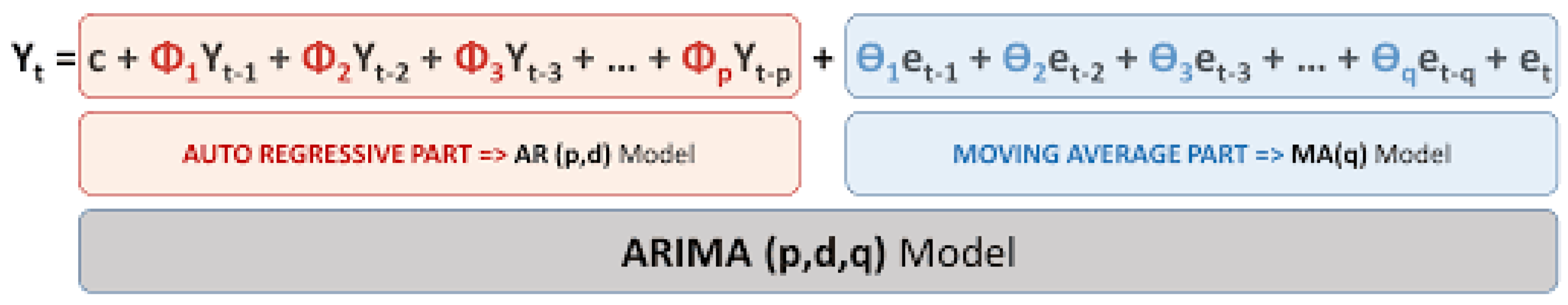
Figure 2.
Chain-like structure of LSTM with gated memory cells.
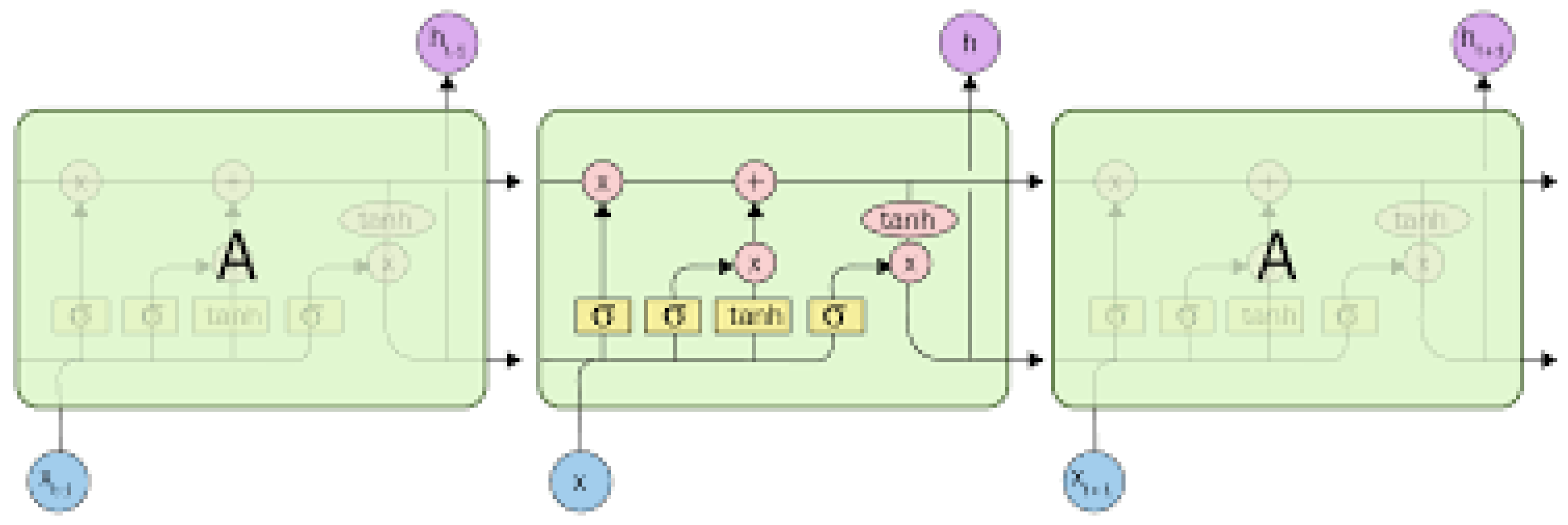
Figure 3.
NVIDIA stock prices before differencing.
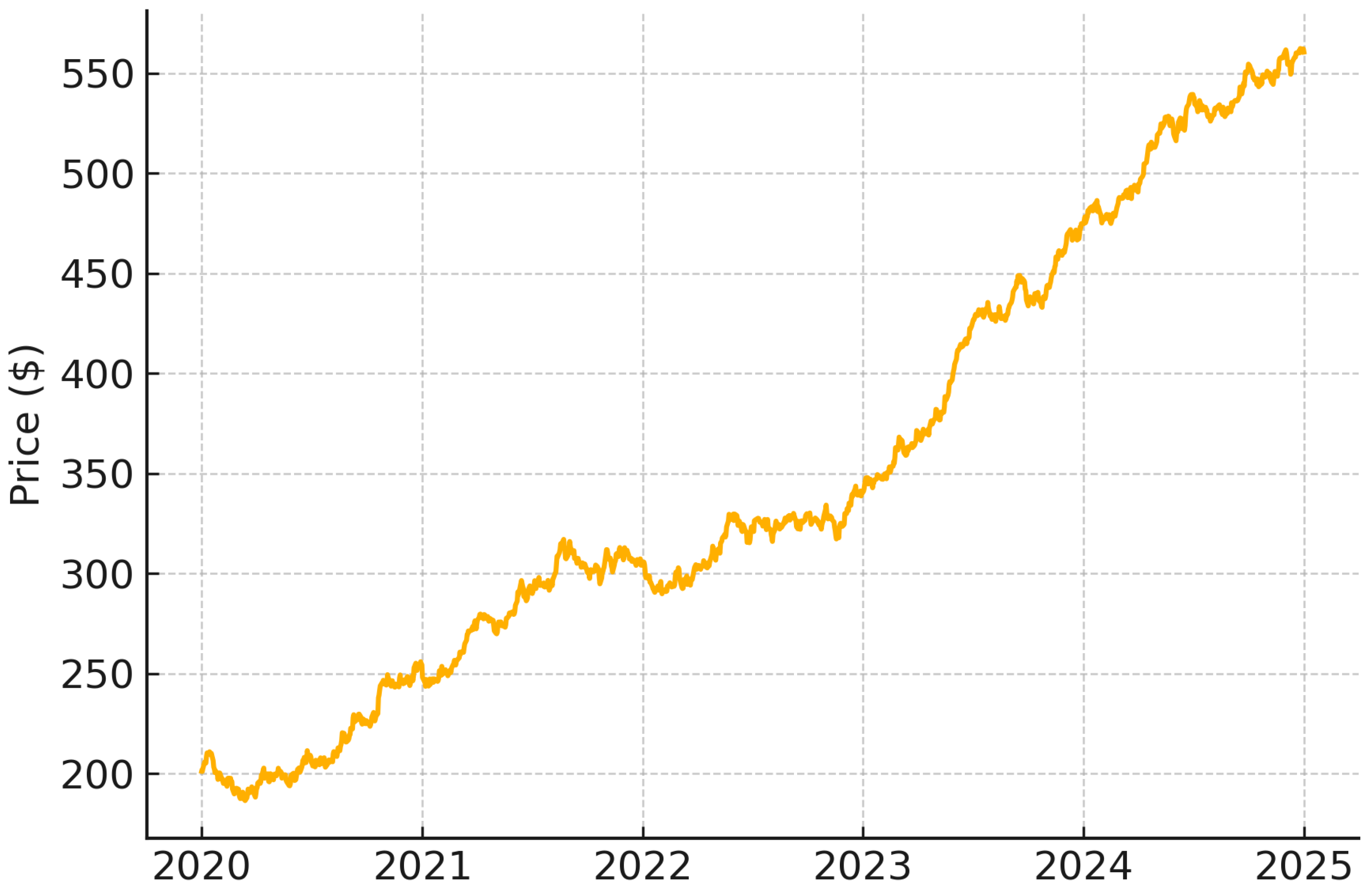
Figure 4.
NVIDIA stock prices after first-order differencing.
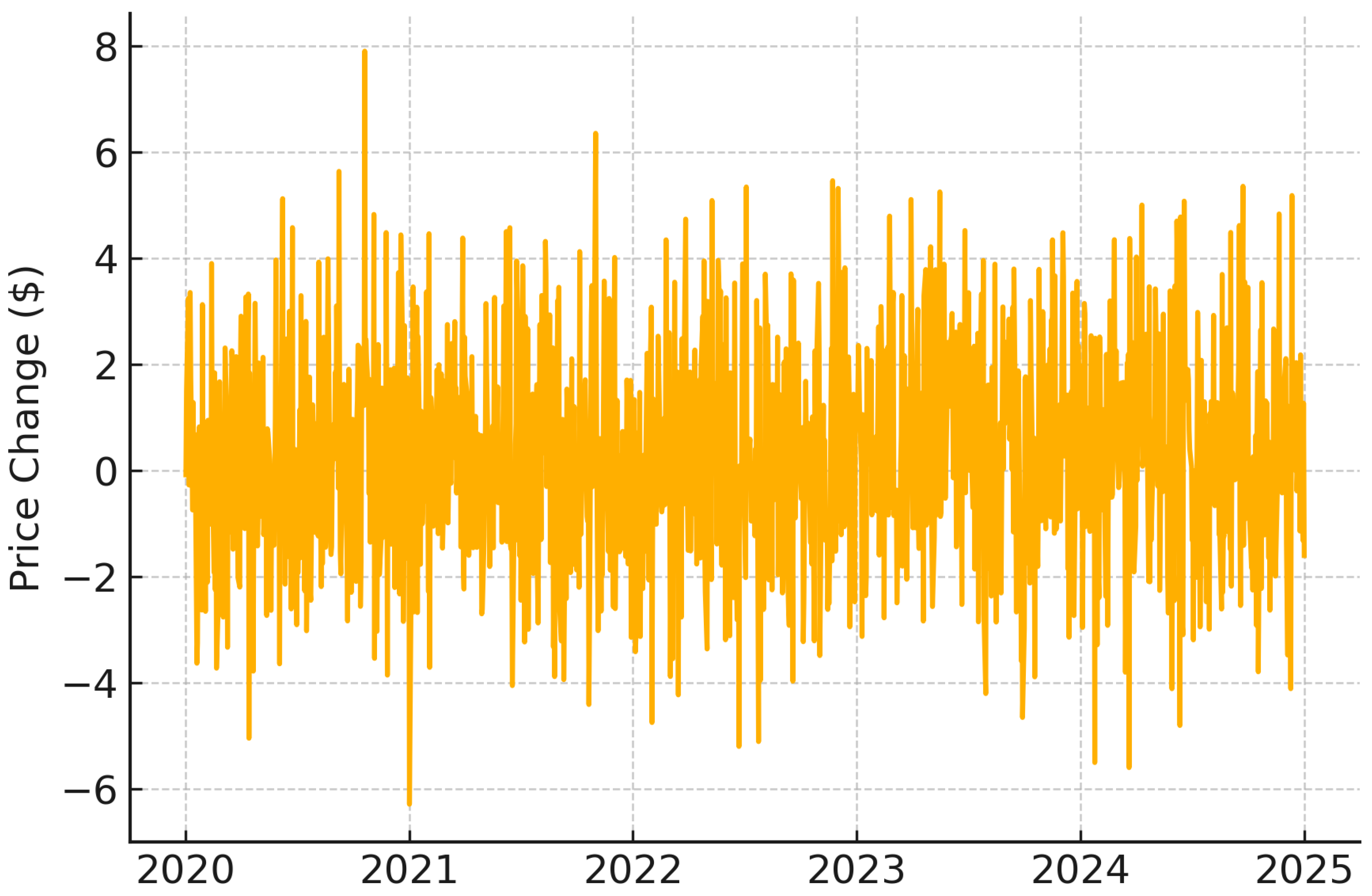
Figure 5.
Sliding window segmentation applied to S&P 500 price data.
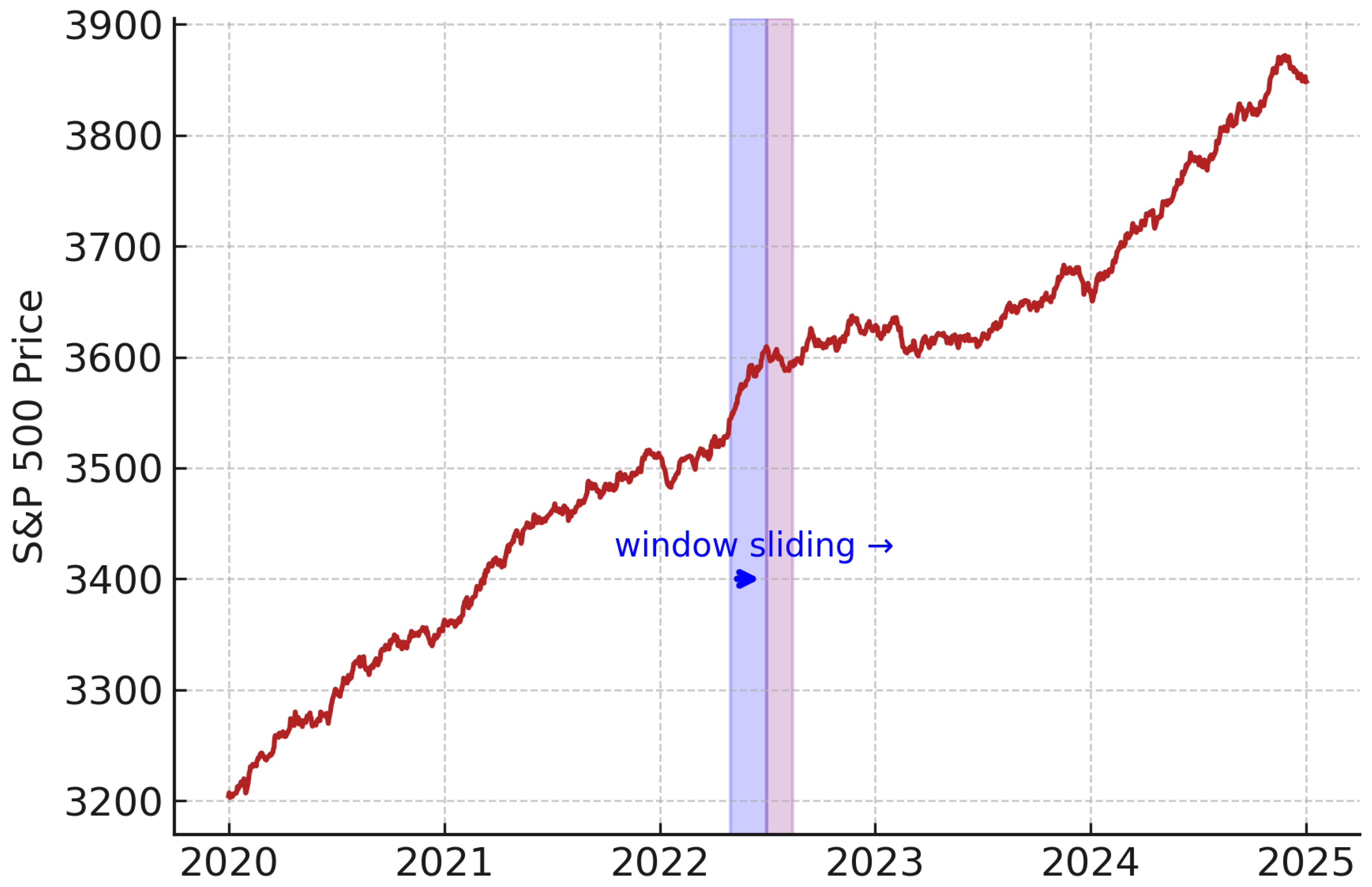
Figure 6.
Prediction performance using non-normalized input data.
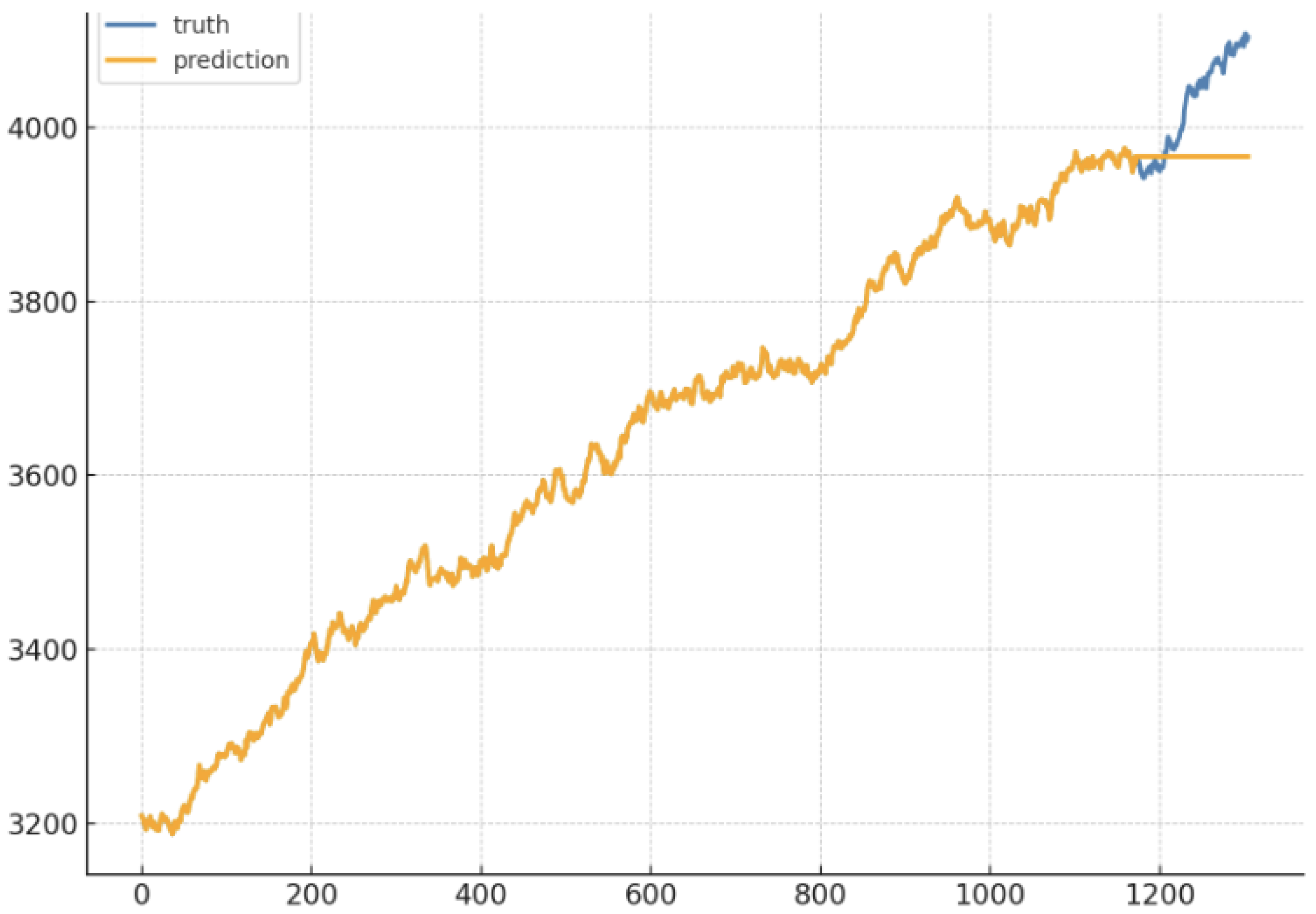
Figure 7.
Multi-Model Forecasting Pipeline.
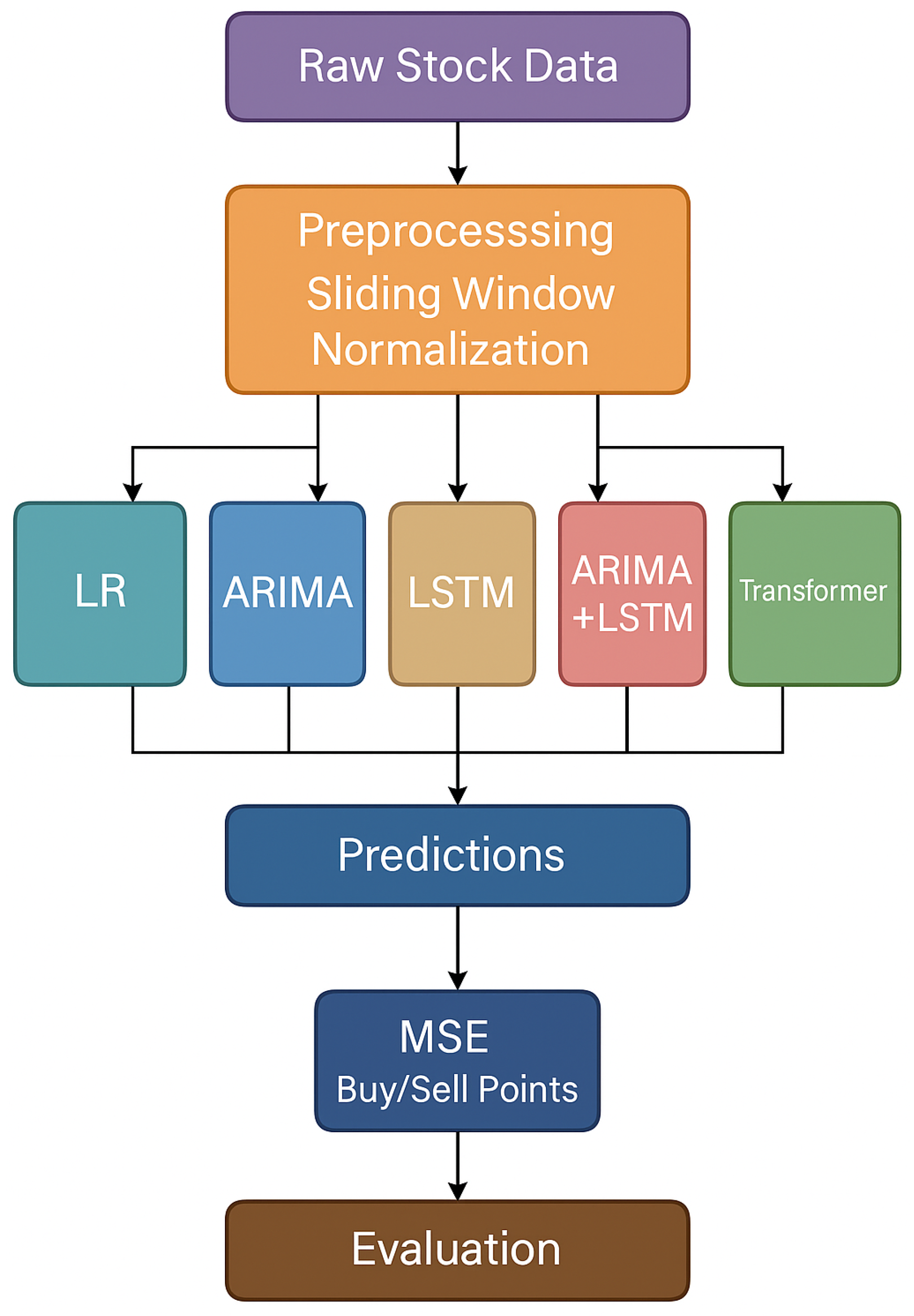
Figure 8.
Cross-Model MSE Heatmap.
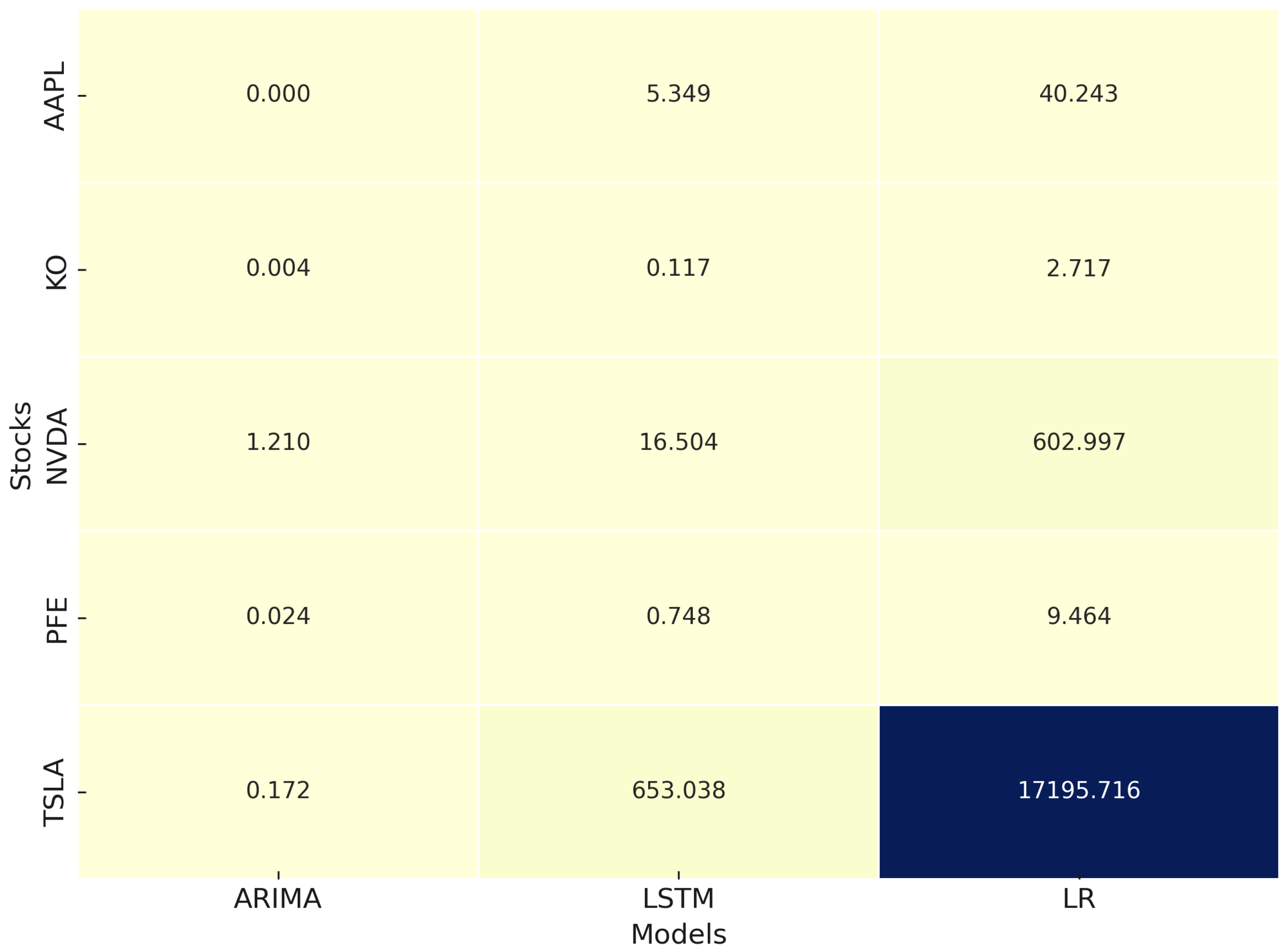
Figure 9.
LSTM Normalization vs Non-Normalization.
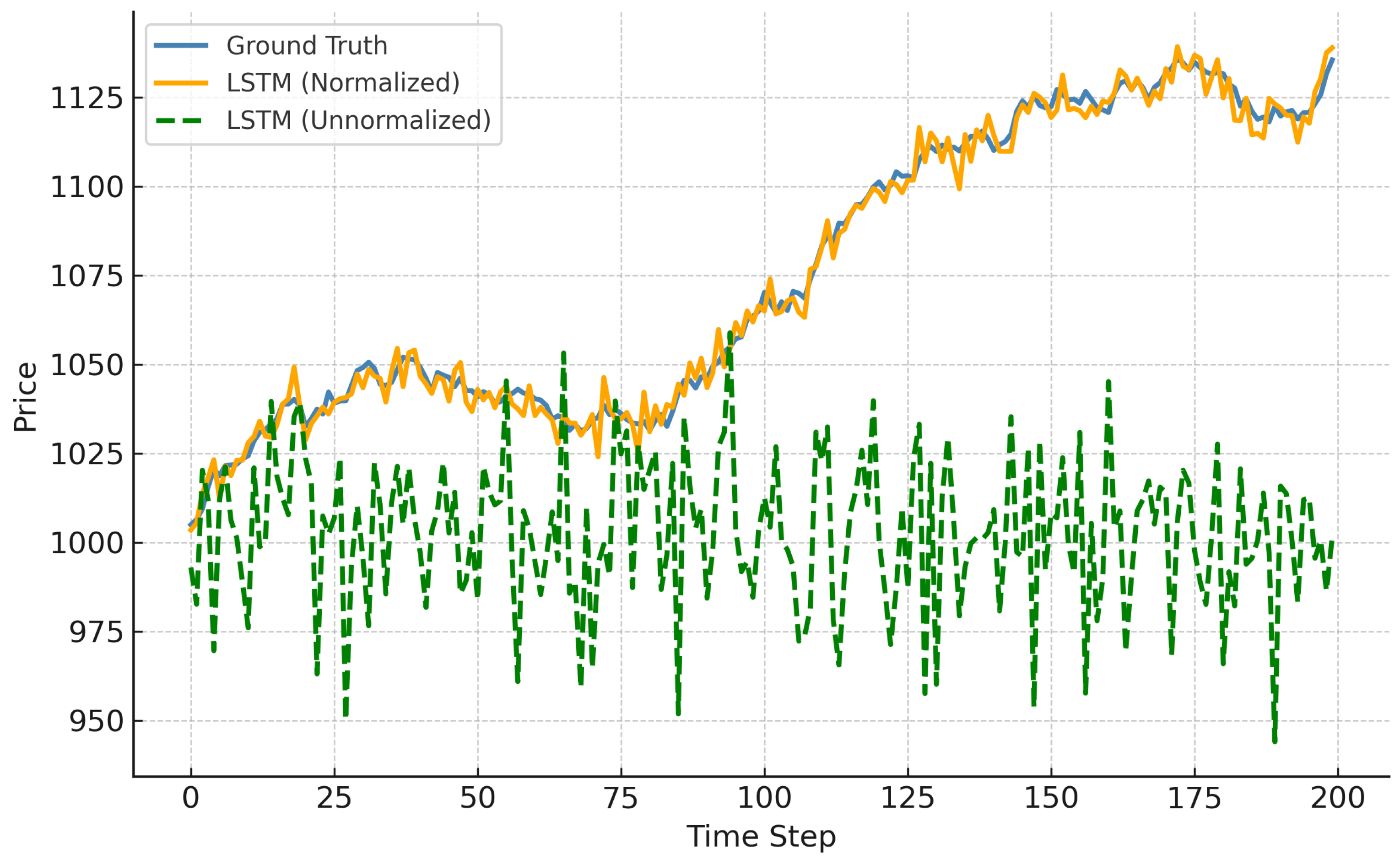
Figure 10.
ARIMA+LSTM Ensemble Prediction Comparison.
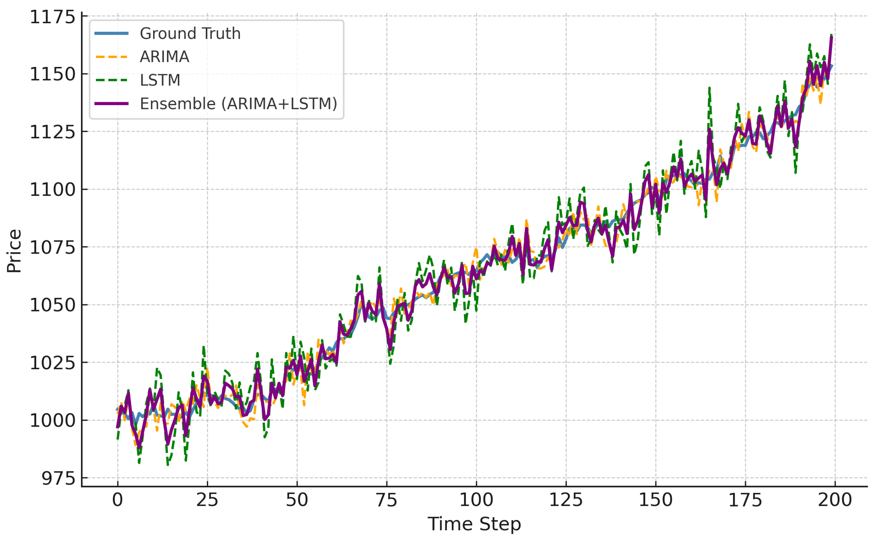
Figure 11.
Transformer vs ARIMA Prediction on KO.
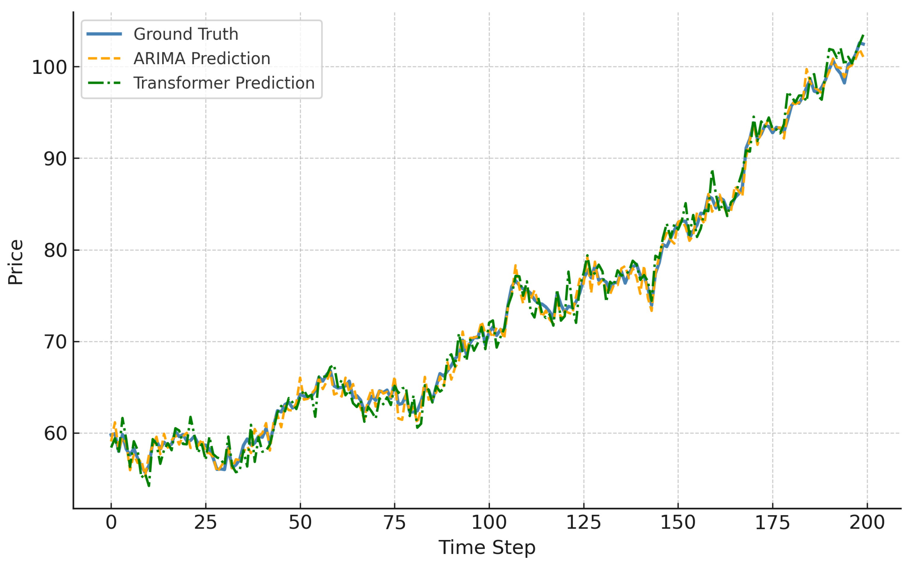

Table 1.
MSE Comparison of Linear Regression under Different Feature Configurations.
| Feature Set | AAPL | KO | NVDA | PFE | TSLA |
|---|---|---|---|---|---|
| 5-day Close Only | 0.021 | 0.004 | 1.340 | 0.028 | 0.170 |
| 5-day Close Only | |||||
| (Full 5 Features) | 0.019 | 0.0035 | 1.210 | 0.024 | 0.172 |
Table 2.
LSTM Performance with Different Architectures and Input Preprocessing.
| Configuration | NVDA(MSE) | TSLA(MSE) |
|---|---|---|
| 1 Layer, 64 Units, No Normalization | 18.4 | 700.5 |
| 2 Layers, 64 Units, No Normalization | 17.8 | 670.2 |
| 1 Layer, 64 Units, Normalized | 1.45 | 160.3 |
| 2 Layers, 64 Units, Normalized | 1.31 | 153.2 |
Table 3.
Best ARIMA Model Parameters and MSE for Each Stock.
| Stock | (p,d,q) Parameters | MSE |
|---|---|---|
| AAPL | (1,1,1) | 0.0004 |
| KO | (0,1,1) | 0.004 |
| NVDA | (2,1,2) | 1.210 |
| PFE | (1,1,1) | 0.024 |
| TSLA | (1,1,0) | 0.172 |
Table 4.
Model Performance Comparison (Including Ensemble and Transformer).
| Stock | ARIMA MSE |
LSTM MSE |
Ensemble (ARIMA+ LSTM) MSE |
Transformer MSE |
|---|---|---|---|---|
| AAPL | 0.0004 | 0.117 | - | 0.005 |
| KO | 0.004 | 0.117 | - | 0.001 |
| NVDA | 1.210 | 16.504 | 1.051 | - |
| PFE | 0.024 | 0.748 | - | - |
| TSLA | 0.172 | 653.038 | 0.161 | - |
Disclaimer/Publisher’s Note: The statements, opinions and data contained in all publications are solely those of the individual author(s) and contributor(s) and not of MDPI and/or the editor(s). MDPI and/or the editor(s) disclaim responsibility for any injury to people or property resulting from any ideas, methods, instructions or products referred to in the content. |
© 2025 by the authors. Licensee MDPI, Basel, Switzerland. This article is an open access article distributed under the terms and conditions of the Creative Commons Attribution (CC BY) license (http://creativecommons.org/licenses/by/4.0/).
Copyright: This open access article is published under a Creative Commons CC BY 4.0 license, which permit the free download, distribution, and reuse, provided that the author and preprint are cited in any reuse.


