
Submitted:
10 January 2025
Posted:
13 January 2025
You are already at the latest version
Abstract
Solar flares, originating from sudden energy releases in the Sun’s atmosphere, pose significant risks to spaceborne and terrestrial technological systems, including satellite operations, communications networks, and power grids. Accurate solar flare forecasting is therefore essential for mitigating these impacts and advancing space weather prediction capabilities. In this study, we present a comprehensive deep-learning-based approach utilizing multi-channel observations from the Solar Dynamics Observatory (SDO), a spaceborne remote sensing platform dedicated to solar monitoring. Our analysis focuses on classifying solar flares under three scenarios: C vs. 0, M vs. C, and M vs. 0, leveraging ten distinct image channels spanning photospheric magnetograms and extreme ultraviolet (EUV) wavelengths. We trained and evaluated three modern convolutional neural network architectures—ResNet50, GoogLeNet, and DenseNet121—using the True Skill Score (TSS) and Gini coefficient to assess performance. The results highlight the superior predictive power of magnetogram data, with additional contributions from EUV channels such as 94 and 211 Å. This work underscores the utility of combining multi-spectral solar observations with state-of-the-art deep learning architectures to capture subtle pre-flare signatures and improve flare prediction accuracy. Furthermore, the methodology and open dataset provide a reproducible benchmark for advancing solar flare forecasting, supporting the broader remote sensing and space weather research communities.
Keywords:
space weather
; solar activity
; convolutional networks
1. Introduction
Solar flares represent sudden, intense brightenings in the solar atmosphere, typically associated with active regions where complex magnetic field configurations store vast amounts of energy [1]. When magnetic field lines become twisted or sheared beyond their threshold, a sudden release of energy occurs—most commonly through a process called magnetic reconnection [2]—leading to dramatic outbursts of radiation across the electromagnetic spectrum and the acceleration of high-energy particles. These explosive events can trigger coronal mass ejections (CMEs) that hurl charged plasma into interplanetary space. Such solar activity not only shapes the heliosphere but also affects space weather conditions near Earth, influencing satellite operations, high-frequency communications, GPS reliability, and power grid stability. Understanding the mechanisms behind solar flares and reliably forecasting their occurrence has therefore become a critical goal for both scientific and practical reasons, as severe flares can induce geomagnetic storms with significant societal and economic impacts [3].
From a data perspective, modern solar observatories—especially space-based missions like NASA’s Solar Dynamics Observatory (SDO)—have revolutionized how researchers monitor and investigate the Sun [4]. Instruments such as the Atmospheric Imaging Assembly (AIA) [5] and the Helioseismic and Magnetic Imager (HMI) [6] capture continuous, high-resolution images in multiple wavelengths, detailing both the magnetic field structures on the photosphere and the coronal plasma above. Meanwhile, complementary datasets (e.g., from GOES X-ray flux measurements [7]) provide insight into the flare intensity and timing. By fusing these observations, scientists can identify key precursors of flare activity—such as changes in magnetic shear, emerging flux regions, or brightening patterns in the corona—and leverage machine learning methods [8] to predict when and where a flare of a certain class (C, M, or X) is most likely to occur. This multifaceted approach, combining physics-based knowledge with computational algorithms, underpins current advances in flare forecasting research [9].
Bridging these fundamental considerations—namely, the physical underpinnings of solar flares, their technological and societal importance, and the variety of data streams now available—researchers have pursued increasingly sophisticated flare prediction methodologies. Early approaches often relied on heuristic assessments of sunspot group complexities or simple threshold-based rules on magnetic features, but the advent of high-cadence observations from space-based telescopes, coupled with modern computational capabilities, has transformed this field. Therefore, in the following sections, we review a series of key studies that showcase how evolving machine learning algorithms and integrated solar observations are being used to improve predictive accuracy and capture the intricate processes that lead to flare eruptions. This progression of work lays the foundation for our own experiments, which seek to refine and extend current forecasting techniques with enhanced data inputs and contemporary deep-learning architectures.
In their paper, Bloomfield and colleagues [10] emphasize the importance of standardized metrics and consistent testing protocols. They argue that reliable comparisons between different prediction algorithms—especially those based on magnetogram data—require uniform data preprocessing, clear definitions of forecast windows, and well-defined performance measures. Their work set a precedent for fair benchmarking, making it easier for the community to evaluate and contrast new methods on an equal footing.
Bobra and Couvidat [8] introduced a machine-learning-based technique that harnessed SDO/HMI vector magnetic field data to predict solar flares. Their study provided one of the earliest demonstrations of how detailed magnetogram information could be leveraged in a supervised classification framework. They showed that specific magnetic features—such as gradients and measures of non-potentiality—significantly enhance the accuracy of forecasts for major flares.
Nishizuka and collaborators [11] expanded on the idea of combining various data sources. By incorporating both ultraviolet emission data (captured in the solar atmosphere) and magnetogram data (from the photosphere), they trained multiple machine-learning algorithms to classify future flare events. Their results underscored the advantages of fusing multiple wavelengths and types of observations, improving the performance compared to single-data-stream methods.
Liu and co-authors [12] concentrated on random forest models to mine SDO/HMI features for flare prediction. Their rigorous evaluation highlighted that even classical algorithms—when carefully tuned—can match or exceed more computationally expensive methods in terms of reliability. They also discussed how specific features from vector magnetic fields (e.g., total unsigned flux, vertical current) could effectively separate flare-productive active regions from quiet ones.
Florios and colleagues [13] presented a broad exploration of magnetogram-derived predictors across different machine-learning techniques. Their work evaluated various classification algorithms—including support vector machines and neural networks—and compared their respective predictive skills. An important contribution was an in-depth look at feature selection, revealing which magnetogram-based metrics are most indicative of imminent flare activity.
Jonas and co-workers [14] demonstrated that combining photospheric and coronal observations could yield improvements in identifying not only major flares but also mid-level events. They underscored the value of including coronal signatures, such as loop structures visible in AIA channels, to capture pre-eruptive processes that might be missed if one focuses solely on surface (photospheric) magnetic fields.
In another work [15] by Nishizuka’s team, they detailed a deep learning architecture designed for near-real-time flare forecasting. Leveraging extensive training data, they showcased how convolutional neural networks (CNNs) can automatically extract pertinent features from ultraviolet and magnetogram images. The proposed system aimed for operational readiness, demonstrating how AI-driven forecasts might be integrated into space weather alert pipelines.
Finally, more recent study by Zhang at al. [16] have sought to refine the synergy between classical statistical techniques and advanced machine learning. By systematically comparing these approaches, authors have highlighted how feature engineering—incorporating physical knowledge of solar activity—remains crucial for robust predictions. Their results underscore the ongoing convergence of domain expertise and modern computational tools in improving flare forecasts.
Over the past decade, numerous studies have advanced our understanding of solar flare prediction by leveraging increasingly sophisticated models, particularly in their ability to analyze magnetic-field data from instruments such as SDO/HMI and complementary coronal observations from SDO/AIA. Yet, existing research often concentrates on a narrower subset of data—commonly vector magnetograms—or relies on smaller, proprietary datasets, limiting comparability and reproducibility.
Furthermore, the range of reported success score - mainly the True Skill Score (TSS) - is strikingly broad, highlighting substantial variability in experimental setups and data utilization. For instance, the efficiency of predicting >M-class flares, as measured by the TSS, spans values such as 0.81 [8], 0.9 [11], 0.5 [12], 0.74 [13], 0.84 [14], and 0.8 [15]. This wide disparity underscores the challenges posed by differences in dataset composition, feature selection, and prediction window definitions across studies. For instance, some studies utilize time-dependent sequences of magnetic and EUV data, while others rely solely on static snapshots or derived quantities, such as magnetic shear or total unsigned flux. Additionally, the prediction windows used by algorithms vary considerably, spanning from minutes to hours or even days before the forecasted event.
These inconsistencies make it difficult to draw direct comparisons between methods or to reliably assess the impact of specific data choices, preprocessing techniques, or algorithmic improvements on prediction performance. Without a standardized approach to dataset division, prediction window selection, and input feature definition, progress in solar flare forecasting risks being fragmented, with individual advances difficult to integrate into a cohesive framework for broader community use. This underscores the need for open datasets, consistent evaluation protocols, and reproducible methods to establish a solid foundation for benchmarking and improving predictive capabilities.
At the same time, the rapid progress in deep learning architectures has opened up fresh opportunities to combine high-resolution images across multiple wavebands, revealing predictive cues not always captured by magnetogram-based features alone. These developments underscore both the need and the potential for a new, more comprehensive experiment that (i) integrates state-of-the-art convolutional neural networks and other deep structures, (ii) broadens the data inputs to include various SDO channels beyond vector magnetic fields, and (iii) employs an open benchmark dataset that other researchers can adopt for transparent comparison. In the following sections, we present such an experiment—designed to offer not only fresh insights into the predictability of mid-range (C-class) and strong (M-class) flares, but also a foundation for replicable, community-driven progress in solar flare forecasting.
2. Dataset Description
Our analysis is based on the publicly available SDOBenchmark1 database developed by Roman Bolzern and Michael Aerni from Institute for Data Science, Switzerland. It consists of 9,220 samples recorded from January 2012 through December 2017. Each sample is associated with an active region (AR), yielding a total of 1,182 unique ARs across the entire dataset. Each sample covers a 12-hour interval (observation data) recorded before the 24-hour interval (evaluation data) within which the maximum X-ray flux is measured to determine the flare class. Within each observation period, we include SDO images of the AR at -12h, -5h, -1.5h, and -10min relative to the start of the 24-hour window. The images obtained by the SDO and used in this dataset include the following channels: 94Å, 131Å, 171Å, 193Å, 211Å, 304Å, 335Å, 1700Å, continuum and magnetogram.
The peak flux in evaluation period ranges from (minimum) to (maximum), with a mean of and a standard deviation of . To separate samples into distinct flare classes, we adopt the following thresholds:
- Class 0, quiet Sun : peak flux < ,
- Class 1, C-class events: peak flux ,
- Class 2, M- or X-class events: peak flux.
As summarized in Table 1, the dataset is imbalanced, with approximately 50% of the samples falling into Class0, whereas only 514 instances instances (about 5%) belong to Class2, representing the most intense flares. This imbalance underscores the need for methods that can handle skewed distributions, for example through class weighting or by employing metrics robust to minority-class scarcity. The dataset is divided into training and test sets; in the test set, the imbalance is mitigated to ensure more comparable numbers of events per class. Furthermore, the active regions (ARs) in the training and test sets do not overlap (ARs in training: 1091, ARs in test: 91), preventing the model from seeing the same AR during both training and inference.
Figure 1 illustrates the distributions of peak flux values, plotted with a logarithmic scale on the vertical axis due to the large variation in flux. Meanwhile, Figure 2 shows the distributions of samples across the three flare classes, confirming that Classes 0 and 1 dominate, whereas Class 2 contains comparatively fewer observations.
In addition, we examined the temporal coverage by grouping samples according to their start timestamps on a monthly basis. As depicted in Figure 3, the dataset is relatively well-distributed over the period from early 2012 to late 2017, allowing for potential studies of solar cycle effects on flare productivity.
Overall, these data provide a valuable opportunity to investigate flare forecasting across a broad range of intensities, from quiet-sun conditions (Class 0) to strong and extreme events (Class 2). However, any modeling approach must account for the class imbalance and the wide dispersion in values. In the following sections, we discuss how we leverage these observations and deep learning methodologies to address these challenges in solar flare prediction.
3. Experiment
To evaluate how well deep neural networks could differentiate among flare classes using multi-channel SDO observations, we designed an extensive experiment comprising three classification scenarios—C vs. 0, M vs. C, and M vs. 0—across ten distinct image channels (94, 131, 171, 193, 211, 304, 335, 1700, continuum, and magnetogram). For each scenario and channel, we trained three different state-of-the-art deep-learning architectures—ResNet50[17], GoogLeNet[18], and DenseNet121[19]—resulting in a comprehensive comparison of models and data modalities. The models thus act as binary classifiers, predicting flare class from four images (acquired at -12h, -5h, -1.5h, and -10min) obtained from the selected SDO channel. When training a network to distinguish between e.g., M and 0 class, we use in both training and test only the samples of these two classes, so the events of class C are omitted.
All networks were implemented in Python using PyTorch. The code employed a consistent pipeline for dataset loading, model training, validation, and performance logging. We intentionally avoided image transformations such as horizontal and vertical flips during data augmentation. Active regions on the Sun often exhibit features tied to their orientation relative to the solar disk and the north-south axis, and applying such flips could obscure or distort these directional characteristics, potentially degrading the model’s ability to learn meaningful spatial patterns. Each network was initialized with random weights and trained for 50 epochs, with five independent training runs (“retries”) per architecture-channel combination to assess result stability. We used a batch size of 16 and the Adam optimizer (initial learning rate in the range of to , depending on the model) with weight decay=0.01. For the loss function, we used BCEWithLogitsLoss with the ‘pos.weight’ (PyTorch) parameter reflecting the ratio of negative to positive samples, thus mitigating class imbalance in each scenario.
Throughout training, each epoch involved a forward pass over the training set followed by a validation step. We tracked TSS (True Skill Score) and Gini (computed from the ROC AUC) on the validation set for every epoch. If the TSS in validation improved beyond the current best, we saved a checkpoint of the model. This allowed us to retain the best-performing network parameters for each of the five runs.
Data preparation and training were performed on a high-performance NVIDIA A6000 GPU (48 GB VRAM), a cutting-edge hardware resource designed for demanding machine-learning tasks. Despite its advanced capabilities, the experiments required continuous operation for more than five months to complete, highlighting the computational intensity of this study (one epoch - training and validation - took up to 30 min.; total: 3 architectures × 10 SDO channels × 50 epochs × 5 training retries). This extensive processing consumed approximately 400 kWh of energy, underscoring both the scale of the experiment and the challenges of analyzing such a large and complex dataset. We stored outcomes (TSS, Gini, and additional metrics) in serialized Python objects (.pkl files), ensuring reproducibility and enabling offline analysis of the results. This setup provided a rigorous examination of how architectural choice, input channel, and classification scenario interact in flare forecasting, while also highlighting the utility of advanced training strategies and balanced loss functions for robust performance across diverse solar conditions.
4. Performance Metrics
In this study, we employ two complementary metrics to assess model performance: the True Skill Score (TSS) and the Gini coefficient. TSS is widely used in meteorological and space weather contexts to evaluate classification skill under imbalanced conditions [20,21], while Gini provides a threshold-independent measure of rank-order discrimination [22].
TSS, also referred to as the Peirce Skill Score or the Hanssen–Kuipers discriminant [20,23], is defined for a binary classification task by:
where is the number of true positives, is the number of true negatives, is the number of false positives, and is the number of false negatives. In solar flare forecasting, positive labels typically denote flaring events (e.g., M- or C-class flares), while negative labels correspond to non-flaring or weaker-flare samples. A TSS of indicates perfect discrimination, 0 corresponds to random (no-skill) classification, and values below 0 imply worse-than-random performance. One key advantage of TSS is its robustness to class imbalance: it balances both the hit rate (sensitivity) and correct rejections (specificity), thus ensuring that a large disparity in positive versus negative samples does not excessively skew the score [21].
The Gini coefficient, in turn, measures how effectively a classifier ranks samples from most likely to least likely to be positive, regardless of a particular decision boundary. It is related to the area under the Receiver Operating Characteristic (ROC) curve () via:
following the definition in [22]. An AUC of denotes perfect rank ordering, hence . Conversely, an AUC of (random ordering) yields , and negative values imply an ordering worse than random.
In practice, using both TSS and Gini provides a more comprehensive evaluation of model behavior. TSS highlights performance at an optimal decision threshold, demonstrating how effectively the classifier separates flaring from non-flaring samples in the best operational setting. However, it does not account for how sensitive the performance is to small changes in this threshold, which could potentially lead to a significant reduction in efficiency. In contrast, the Gini coefficient offers a threshold-independent perspective, verifying that strong results are not confined to a single decision point but are consistent across the entire range of possible thresholds. This dual evaluation is particularly valuable in flare prediction, where class imbalance and diverse operational requirements make reliance on a single metric insufficient. Unfortunately, the Gini coefficient is not widely used in solar flare forecasting, making it difficult to determine whether the high efficiency reported by existing classifiers holds across thresholds other than the optimal one.
5. Results
We present two sets of composite plots (Figure 4 and Figure 5) illustrating the results for TSS and Gini, respectively. In the first figure (TSS), we use a 3x3 grid of boxplots, with each row representing one of the three classification scenarios (C vs 0, M vs C, M vs 0) and each column corresponding to one of the deep-learning architectures (ResNet50, GoogLeNet, DenseNet121). The boxplots depict the distribution of TSS obtained over multiple (5) experimental runs, thereby highlighting both the central tendencies and variabilities in performance for each combination of scenario and architecture.
In the second figure (Gini), we employ the same layout, again with the three rows depicting the different classification tasks and the three columns covering the same set of neural networks. Here, the Gini values are plotted using boxplots in an identical configuration, enabling a direct comparison against the TSS results. To further facilitate such comparisons, the axes in both figures have been aligned to the same scale, ensuring a consistent reference for visually assessing performance across the two metrics.
The corresponding numeric tables: Table 2, Table 3 and Table 4 show the average, standard deviation and maximum values (in parethesis) of the obtained coefficients results.
Across all three scenarios—C vs. 0, M vs. C, and M vs. 0—the mean and maximum scores suggest that magnetogram data (i.e., photospheric magnetic-field information) remain the most predictive. Channels such as 94 and 211 (extreme-ultraviolet emissions) often follow closely, whereas 171 and 1700 tend to yield lower values. This pattern highlights the strong connection between magnetic-field complexity and flare productivity, particularly for mid- to high-energy flares (C- and M-class).
Interestingly, in many cases, DenseNet121 outperforms or ties with GoogLeNet and ResNet50, especially when analyzing the highest scores (i.e., maximum TSS or Gini across multiple training retries). However, the differences among these three architectures are not drastic. This narrow performance gap implies that the choice of which deep neural network to deploy may be less critical than how the data are prepared or which channels are selected. For example, a carefully tuned ResNet50 using a magnetogram might still surpass a poorly tuned DenseNet121 on a less-informative channel.
5.1. Channel Variations
Magnetograms directly capture the photospheric magnetic configurations, which are strongly tied to flare initiation processes such as shearing, flux emergence, or cancellation. EUV channels reveal upper-atmospheric and coronal structures, which, while important, may sometimes lag behind or be less uniquely indicative of imminent flares.
Some EUV wavelengths (e.g., 304 Å, 171 Å) can be more susceptible to brightness saturation or line-of-sight complexities. If a flare region is partially obstructed or if the brightening is relatively mild (for C-class flares, for instance), the signal might not be as sharply defined in these channels as in 94 Å or 211 Å.
The performance gap between magnetograms and continuum images (1700 Å, visible continuum) suggests that purely photospheric brightness patterns are less indicative of flare readiness than direct measurements of magnetic flux. Continuum images primarily track thermal emission from the lower photosphere, which may not significantly change until the flare is underway.
5.2. Scenario-Specific Observations
The M vs. 0 classification—distinguishing moderate flares from a quiet Sun—shows the highest TSS (often exceeding 0.80) and Gini (0.90+). The large contrast between active regions producing M-class flares and regions with no flare activity presumably makes the classification easier. This outcome aligns with physical intuition: an M-class flare requires strong, complex magnetic fields, easily distinguishable from the very minimal magnetic gradients typical of a quiet Sun. High TSS and Gini both indicate that the models can simultaneously achieve accurate classification and robust ranking of cases across a range of thresholds.
In C vs. 0 scenario, TSS mostly lies in the 0.40–0.60 range, while Gini tends to cluster around 0.60–0.70. That drop compared to M vs. 0 reflects the fact that C-class flares can emerge from less dramatic field configurations and more modest brightening patterns, making them harder to differentiate from quiet conditions. The borderline energy levels for C-class flares can resemble enhanced active regions that do not necessarily erupt. Thus, while the classification still achieves moderate success, both TSS and Gini reveal noticeable overlap between positive (C-class) and negative (quiet Sun) samples.
Attempting to separate two flare classes, M vs. C, is often the most challenging, with TSS frequently peaking around 0.57–0.59, and Gini near 0.70–0.72. Physically, M- and C-class flares can share many precursor signatures (e.g., increased coronal loop structures or moderate magnetic shear). Although M-class flares are inherently stronger, the observable differences prior to peak emission can be subtle, especially in EUV channels. Magnetograms again lead, but even they struggle to consistently discriminate between moderate (C) and more intense (M) flares.
5.3. Comparing TSS and Gini
In all scenarios, TSS and Gini show strong mutual agreement regarding which channels and which architectures perform best. Channels with higher TSS consistently exhibit higher Gini.
TSS emphasizes balanced accuracy by accounting for both true positive rate and true negative rate. It is particularly valued for handling unbalanced data (e.g., relatively few intense flares vs. many quiet instances). A TSS of 1.0 would indicate perfect classification; values above 0.80, as seen in some M vs. 0 cases, suggest a highly reliable prediction.
Gini measures ranking ability across all possible decision thresholds. A high Gini >0.90, as observed in M vs. 0 magnetogram cases, implies the model can effectively sort flaring vs. non-flaring instances from the most likely to the least likely, even if the exact threshold is not known a priori.
By jointly examining TSS (i.e., threshold-based accuracy) and Gini (i.e., threshold-independent ranking), we obtain a more holistic view of model performance. A model with strong TSS but modest Gini could indicate that it performs well at one particular threshold but lacks consistent discrimination across other thresholds. Conversely, a high Gini but only moderate TSS might mean that the model sorts the cases well overall but does not pinpoint an optimal decision boundary. In these experiments, the metrics reinforce each other: improved classification is accompanied by better ranking, reflecting robust predictive capabilities in those scenarios.
Our results demonstrate that the maximum True Skill Score (TSS) achieved in our experiments, reaching up to 0.86, compares favorably against previously reported values in the literature for predicting >M-class flares. Automated methods, such as those in [8,11], and [13], report TSS values ranging from 0.5 to 0.9 depending on the dataset and approach used. These results highlight the competitiveness of our method within the landscape of machine-learning-based flare forecasting.
Furthermore, when compared to human expert-based forecasting, our model exhibits clear advantages. Forecasting centers such as NICT and SIDC reported TSS values of 0.21 and 0.34, respectively, for >M-class flares over extended periods [24,25]. This significant gap underscores the potential of advanced deep-learning models to enhance solar flare forecasting beyond traditional, human-reliant methods.
However, it is important to note the inherent challenges in directly comparing TSS values across different studies. Variations in dataset composition, feature sets, prediction windows, and experimental methodologies mean that such comparisons must be interpreted with caution. For instance, while some models use carefully curated and time-synchronized datasets, others may include overlapping training and test events, artificially boosting TSS. Similarly, human forecasting methods often rely on subjective knowledge and experience, which are not directly comparable to algorithmic approaches. Despite these limitations, our results indicate that state-of-the-art deep-learning architectures provide a promising avenue for improving both the reliability and accuracy of solar flare predictions.
Limitations of the Present Experiment and Future Directions
A variety of factors may further explain or constrain our findings, and highlight the potential for extending this research in meaningful ways. First, the current models treat each 12-hour segment in near-isolation, largely overlooking the finer temporal evolution of magnetic structures and EUV signals that can evolve on shorter or more extended timescales. Incorporating multi-temporal or sequence-based data could reveal additional precursors—such as small-scale magnetic flux cancellations or intermittent coronal brightenings—that might improve the model’s performance in borderline cases, particularly for scenarios like C vs. 0 or M vs. C.
Second, the issue of imbalanced classes remains a persistent challenge. While TSS and Gini are more robust to such imbalance than standard accuracy metrics, the rarity of certain flare classes (for instance, a small number of M flares compared to the abundance of non-flaring or weakly flaring instances) can still skew the models. Techniques such as oversampling minority classes, selective data augmentation, or employing specialized loss functions (e.g., focal loss) could further refine the predictive capabilities and better address subtle flare distinctions.
Third, because our dataset spans roughly six years, assessing model generalizability over multiple solar cycles would offer a deeper test of robustness. Flare frequency and magnetic complexity can vary markedly with the solar cycle, and confirming that these methods perform well under different levels of solar activity would strengthen the case for operational adoption. By addressing each of these limitations—temporal resolution, class imbalance, data fusion, and expanded coverage—future research can more effectively refine both the classification (TSS) and ranking (Gini) aspects of flare prediction, and potentially shed further light on the underlying solar dynamics that drive these energetic events.
Lastly, although magnetogram data consistently provides the highest predictive value, opportunities remain to enhance performance by combining multiple channels. Feature fusion or ensemble-based approaches that jointly leverage information from AIA and HMI could help capture a wider spectrum of precursor signatures—particularly in cases where the magnetic field appears only moderately stressed, yet specific EUV emissions signal an imminent flare. This approach holds significant potential for improving predictions, as it could exploit complementary information from different wavelengths, capturing both magnetic field dynamics and coronal plasma activity.
However, the computational cost of such experiments poses a major challenge. Our current experiment, which evaluated individual channels independently, required approximately five months of continuous computation on a state-of-the-art NVIDIA A6000 GPU. Extending this analysis to even pairs of channels would lead to an exponential increase in the number of model configurations and training cycles, potentially pushing the computational time into years. Given these constraints, we deliberately focused on single-channel experiments, designing the study to balance computational feasibility with scientific value.
Future work could address this limitation by leveraging the insights presented here to identify the most promising channel combinations for targeted experiments. For instance, pairing magnetograms with high-performing EUV channels such as 94 or 211 Å may offer the greatest potential for improvement while keeping computational costs manageable. Additionally, advances in multi-GPU systems or distributed computing could enable more comprehensive experiments in subsequent studies, allowing for the exploration of multi-channel data fusion without the prohibitive time constraints observed in this study. By prioritizing single-channel analysis, we have established a foundational benchmark that paves the way for more focused and efficient multi-channel approaches in future research.
6. Conclusions
Solar flares remain one of the most significant drivers of space weather, impacting satellite communications, GPS reliability, and even terrestrial power grids. Motivated by their high societal and technological relevance, we designed an extensive experiment to evaluate how different state-of-the-art deep-learning architectures respond to multi-channel observations from the Solar Dynamics Observatory. Our dataset, spanning six years and targeting various flare classes (C, M, and quiet Sun conditions), enabled a thorough comparison across scenarios—C vs. 0, M vs. C, and M vs. 0. In doing so, we not only assessed traditional metrics like the True Skill Score (TSS), but also examined the Gini coefficient to gauge the models’ ability to rank flaring vs. non-flaring events independently of a single decision threshold.
From the results, we observe that magnetogram data consistently provide the most robust predictive signal, a finding that underscores the vital role of photospheric magnetic structures in initiating flares. Our analyses also confirm that distinguishing M-class flares from quiescent conditions proves comparatively easier than separating lower-level (C-class) events from the quiet Sun, or moderate M-class from C-class flares with less dramatic magnetic signatures. Furthermore, DenseNet121 often yields slightly higher peak performance, though the margins over GoogLeNet or ResNet50 remain modest. By considering both TSS and Gini, we gained a clearer sense of each model’s classification accuracy and its overarching ranking power, ensuring that strong performance was not confined to a singular operating threshold.
Overall, this study reinforces the importance of carefully chosen data channels and highlights how modern convolutional networks can capture subtle flare precursors. It also opens the door to future investigations that incorporate time-series analyses, advanced data fusion, or new architectures adapted to complex solar physics. As solar flares continue to threaten critical systems on Earth and in space, improving flare forecasts remains essential. Our work demonstrates how next-generation deep-learning methods, supported by multi-channel solar observations, can significantly advance this goal.
Moreover, because the validation dataset is publicly accessible and the deep-learning architectures employed here are both contemporary and widely adopted, this work can serve as a consistent benchmark for comparing future methods. Researchers worldwide can thus replicate our experiments, enrich the input data (e.g., by adding other spectral channels), or apply novel network designs—offering a transparent framework that fosters community-driven advancements in solar flare forecasting.
Funding
Authors acknowledge support from the Polish Ministry of Science and Higher Education funding for statutory activities BKM-615/Rau-11/2023.
Conflicts of Interest
The authors declare no conflict of interest.
References
- Shibata, K.; Magara, T. Solar Flares: Magnetohydrodynamic Processes. Living Reviews in Solar Physics 2011, 8, 1–99. [Google Scholar] [CrossRef]
- Priest, E.R.; Forbes, T.G. The magnetic nature of solar flares. The Astronomy and Astrophysics Review 2002, 10, 313–377. [Google Scholar] [CrossRef]
- Webb, D.F.; Howard, R.A. The solar cycle variation of coronal mass ejections and the solar wind mass flux. Journal of Geophysical Research 1994, 99, 4201–4220. [Google Scholar] [CrossRef]
- Pesnell, W.D.; Thompson, B.J.; Chamberlin, P.C. The Solar Dynamics Observatory (SDO). Solar Physics 2012, 275, 3–15. [Google Scholar] [CrossRef]
- Lemen, J.R.; Title, A.M.; Akin, D.J.; Boerner, P.; Chou, C.; Drake, J.F.; Duncan, D.W.; Edwards, C.G.; Friedlaender, F.M.; Heyman, G.F.; et al. The Atmospheric Imaging Assembly (AIA) on the Solar Dynamics Observatory (SDO). Solar Physics 2011, 275, 17–40. [Google Scholar] [CrossRef]
- Schou, J.; Scherrer, P.H.; Bush, R.I.; Wachter, R.M.; Couvidat, S.; Rabello-Soares, M.C.; Bogart, R.S.; Hoeksema, J.T.; Liu, Y.; Duvall, T.L.; et al. Design and Ground Calibration of the Helioseismic and Magnetic Imager (HMI) Instrument on the Solar Dynamics Observatory (SDO). Solar Physics 2012, 275, 229–259. [Google Scholar] [CrossRef]
- Garcia, H.A. Temperature and emission measure from goes soft X-ray measurements. Solar Physics 1994, 154, 275–308. [Google Scholar] [CrossRef]
- Bobra, M.G.; Couvidat, S. Solar Flare Prediction Using SDO/HMI Vector Magnetic Field Data wit a Machine-Learning Algorithm. The Astrophysical Journal 2014, 798. [Google Scholar]
- Toriumi, S.; Wang, H. Flare-productive active regions. Living Reviews in Solar Physics 2019, 16. [Google Scholar] [CrossRef]
- Bloomfield, D.S.; Higgins, P.A.; McAteer, R.T.J.; Gallagher, P.T. Toward Reliable Benchmarking of Solar Flare Forecasting Methods. The Astrophysical Journal Letters 2012, 747. [Google Scholar] [CrossRef]
- Nishizuka, N.; Sugiura, K.; Kubo, Y.; Den, M.; ichi Watari, S.; Ishii, M. Solar Flare Prediction Model with Three Machine-learning Algorithms using Ultraviolet Brightening and Vector Magnetograms. The Astrophysical Journal 2016, 835. [Google Scholar] [CrossRef]
- Liu, C.; Deng, N.; Wang, J.T.L.; Wang, H. Predicting Solar Flares Using SDO/HMI Vector Magnetic Data Products and the Random Forest Algorithm. The Astrophysical Journal 2017, 843. [Google Scholar] [CrossRef]
- Florios, K.; Florios, K.; Kontogiannis, I.; Park, S.H.; Guerra, J.A.; Benvenuto, F.; Bloomfield, D.S.; Georgoulis, M.K. Forecasting Solar Flares Using Magnetogram-based Predictors and Machine Learning. Solar Physics 2018, 293. [Google Scholar] [CrossRef]
- Jonas, E.; Bobra, M.G.; Shankar, V.; Hoeksema, J.T.; Recht, B. Flare Prediction Using Photospheric and Coronal Image Data. Solar Physics 2016, 293, 1–22. [Google Scholar] [CrossRef]
- Nishizuka, N.; Kubo, Y.; Sugiura, K.; Den, M.; Ishii, M. Operational solar flare prediction model using Deep Flare Net. Earth, Planets and Space 2021, 73, 1–12. [Google Scholar] [CrossRef]
- Zhang, H.; Li, Q.; Yang, Y.; Jing, J.; Wang, J.T.L.; Wang, H.; Shang, Z. Solar Flare Index Prediction Using SDO/HMI Vector Magnetic Data Products with Statistical and Machine-learning Methods. The Astrophysical Journal Supplement Series 2022, 263. [Google Scholar] [CrossRef]
- He, K.; Zhang, X.; Ren, S.; Sun, J. Deep Residual Learning for Image Recognition. 2016 IEEE Conference on Computer Vision and Pattern Recognition (CVPR), 2015, pp. 770–778.
- Szegedy, C.; Liu, W.; Jia, Y.; Sermanet, P.; Reed, S.E.; Anguelov, D.; Erhan, D.; Vanhoucke, V.; Rabinovich, A. Going deeper with convolutions. 2015 IEEE Conference on Computer Vision and Pattern Recognition (CVPR) 2014, pp. 1–9.
- Huang, G.; Liu, Z.; Weinberger, K.Q. Densely Connected Convolutional Networks. 2017 IEEE Conference on Computer Vision and Pattern Recognition (CVPR) 2016, pp. 2261–2269. 2261. [Google Scholar]
- Peirce, C.S. The Numerical Measure of the Success of Predictions. Science 1884, 4, 453–454. [Google Scholar] [CrossRef] [PubMed]
- Bloomfield, D.S.; Higgins, P.A.; McAteer, R.T.J.; Gallagher, P.T. Toward Reliable Benchmarking of Solar Flare Forecasting Methods. The Astrophysical Journal Letters 2012, 747, L41. [Google Scholar] [CrossRef]
- Gini, C. Variabilità e mutabilità; Studi Economico-Giuridici dell’Università di Cagliari: Cagliari, Italy, 1912. [Google Scholar]
- Hanssen, A.W.; Kuipers, W.J.A. On the Relationship Between the Frequency of Rain and Various Meteorological Parameters. Mededelingen en Verhandelingen van de Koninklijke Nederlandse Meteorologische Instituut 1965, 81, 2–15. [Google Scholar]
- Kubo, Y.; Den, M.; Ishii, M. Verification of operational solar flare forecast: Case of Regional Warning Center Japan. Journal of Space Weather and Space Climate 2017, 7. [Google Scholar] [CrossRef]
- Devos, A.; Verbeeck, C.; Robbrecht, E. Verification of space weather forecasting at the Regional Warning Center in Belgium. Journal of Space Weather and Space Climate 2014, 4. [Google Scholar] [CrossRef]
| 1 |
Figure 1.
Histogram of values (vertical axis in log scale).
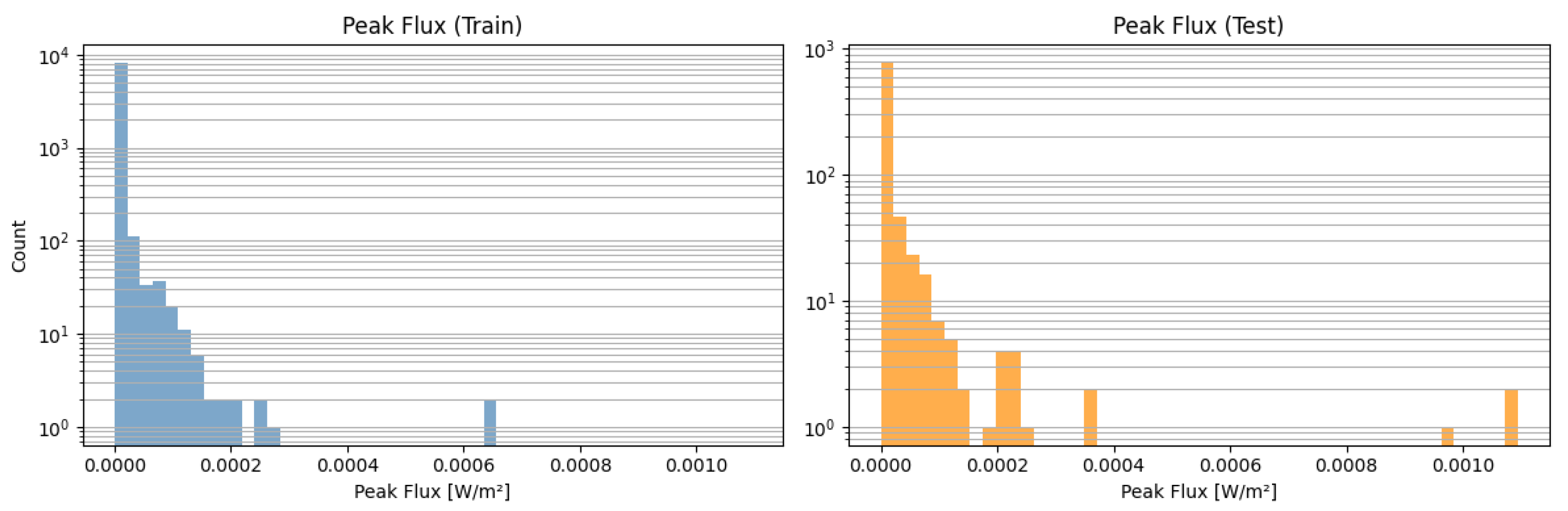
Figure 2.
Histogram of flare classes: 0, 1, 2, and 3.
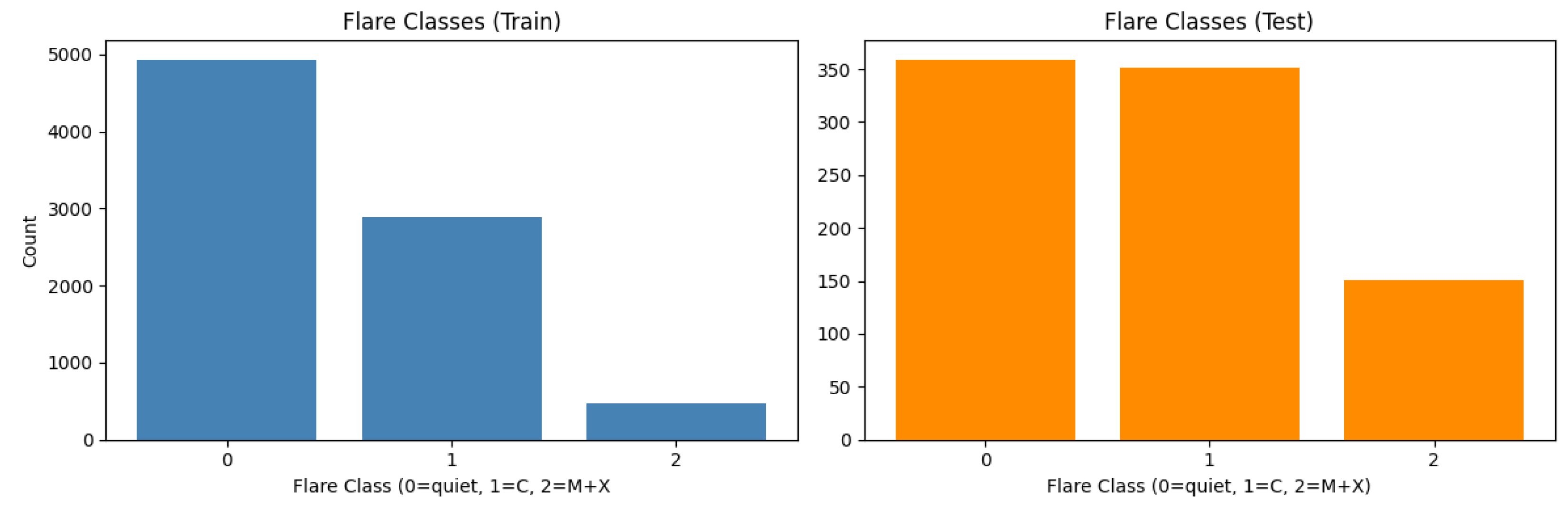
Figure 3.
Number of samples per month between January 2012 and December 2017.
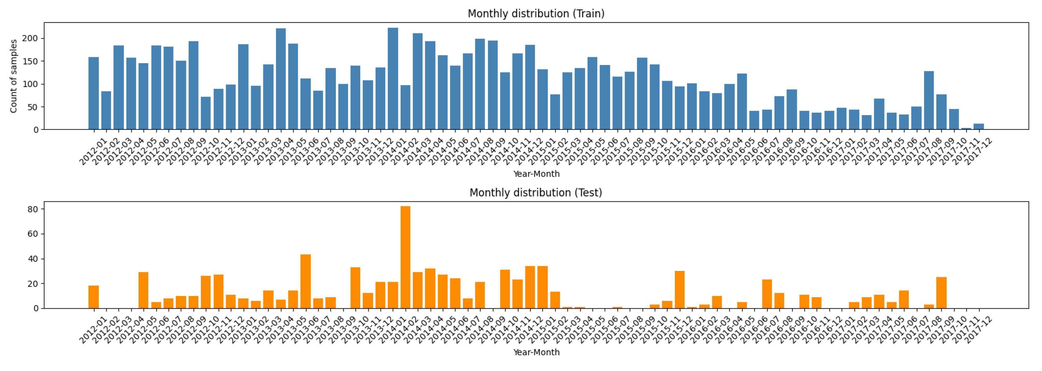
Figure 4.
TSS results.
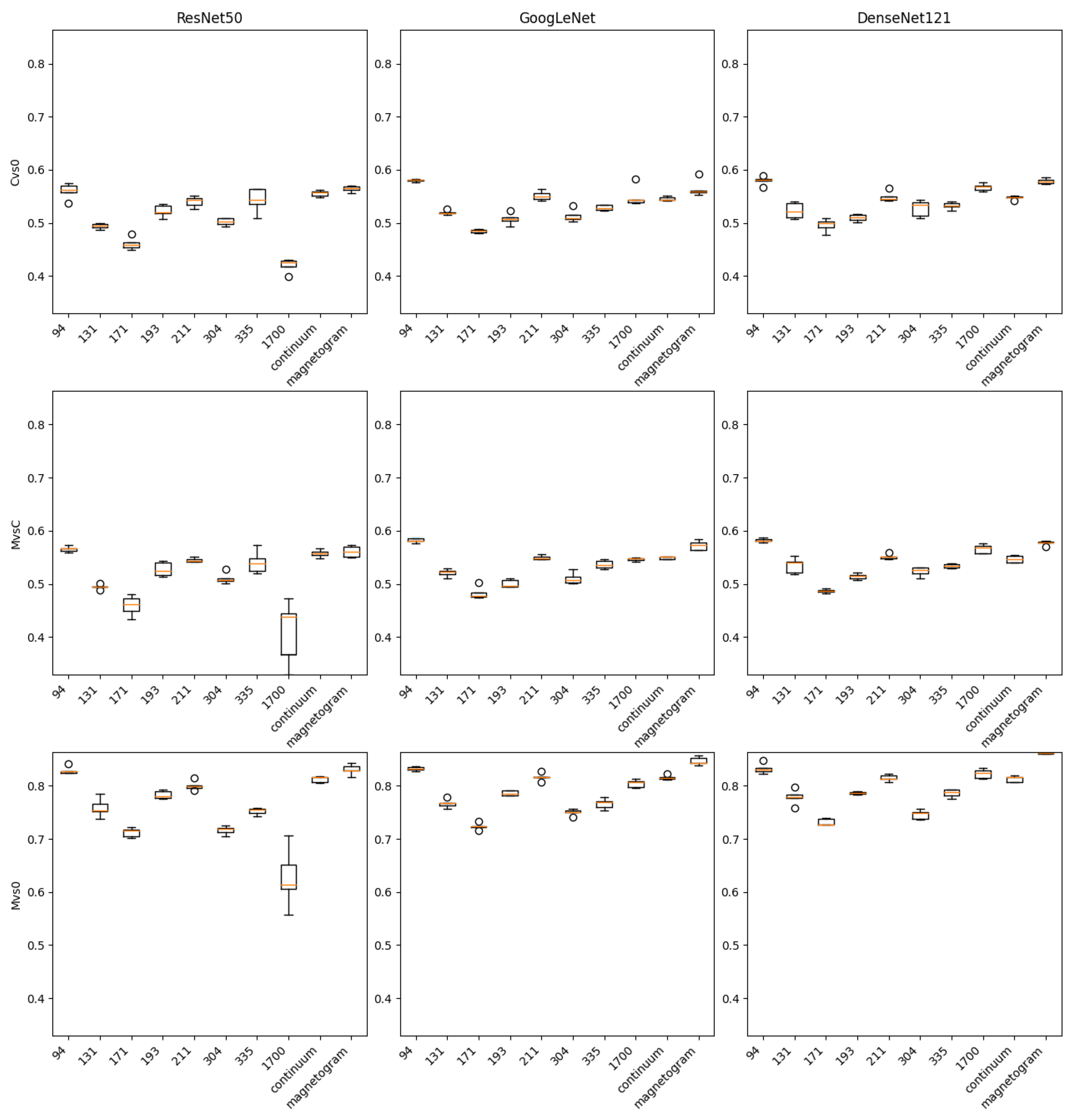
Figure 5.
Gini coefficient results.
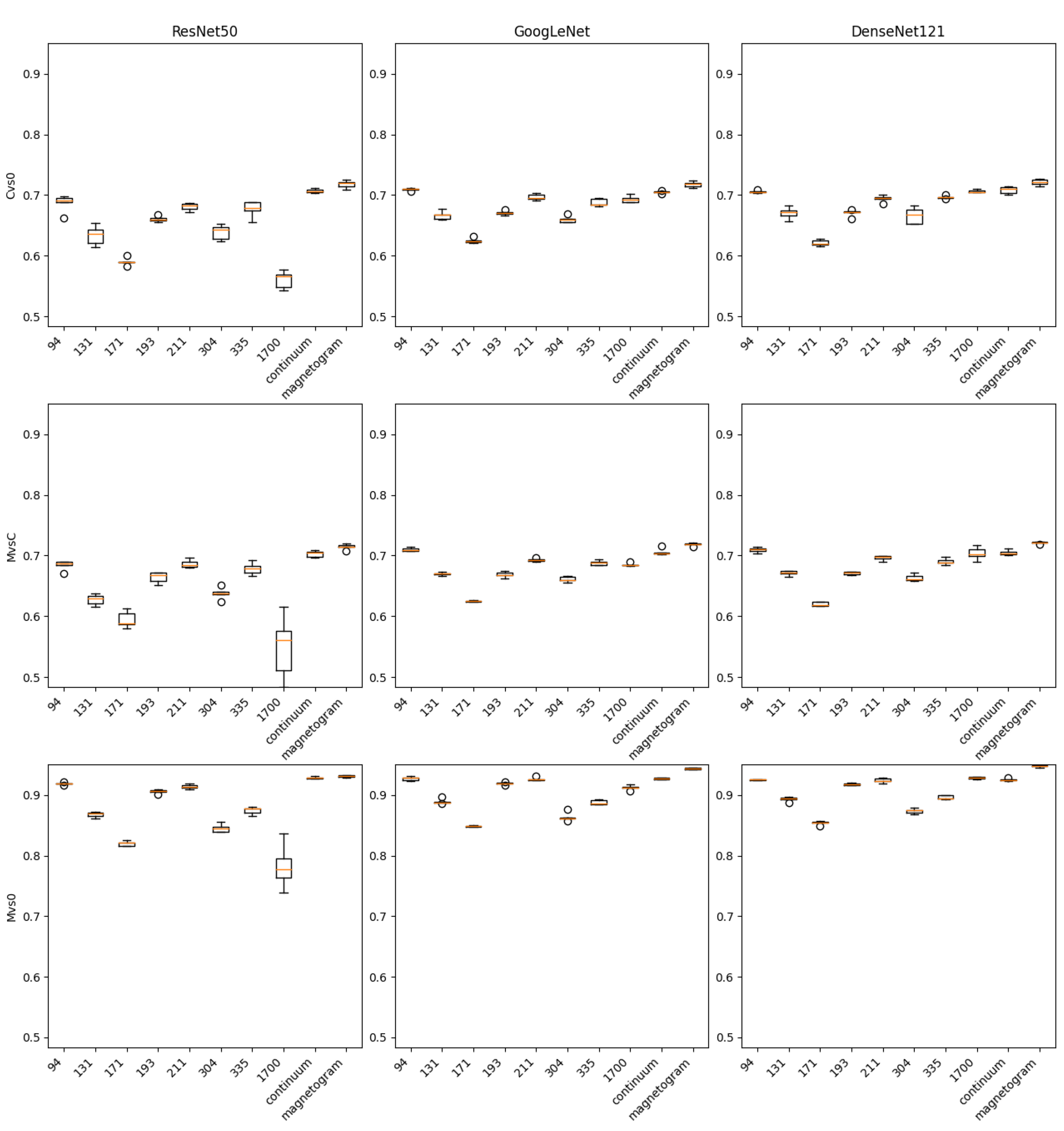

Table 1.
Overview of the SDO-based dataset (2012–2017).
| Parameter | Value |
|---|---|
| Total samples | 9,220 |
| Train, class 0 events (quiet Sun) | 4,930 |
| Train, class 1 events (C-class) | 2,890 |
| Train, class 2 events (M+X-class) | 514 |
| Test, class 0 events (quiet Sun) | 359 |
| Test, class 1 events (C-class) | 351 |
| Test, class 2 events (M+X-class) | 176 |
| Unique active regions (AR) | 1,182 |
| Minimum | |
| Maximum | |
| Mean |
Table 2.
TSS and Gini results for scenario Cvs0.
| Channel | ResNet50 | GoogLeNet | DenseNet121 |
|---|---|---|---|
| 94 | |||
| TSS: | 0.560±0.013 (0.575) | 0.580±0.002 (0.582) | 0.580±0.007 (0.589) |
| Gini: | 0.687±0.013 (0.698) | 0.709±0.002 (0.711) | 0.705±0.002 (0.708) |
| 131 | |||
| TSS: | 0.494±0.004 (0.499) | 0.519±0.003 (0.525) | 0.523±0.013 (0.540) |
| Gini: | 0.633±0.014 (0.653) | 0.667±0.006 (0.677) | 0.671±0.009 (0.683) |
| 171 | |||
| TSS: | 0.461±0.011 (0.479) | 0.485±0.003 (0.488) | 0.496±0.011 (0.509) |
| Gini: | 0.590±0.006 (0.601) | 0.625±0.004 (0.632) | 0.621±0.004 (0.627) |
| 193 | |||
| TSS: | 0.522±0.010 (0.535) | 0.507±0.010 (0.522) | 0.510±0.006 (0.516) |
| Gini: | 0.661±0.004 (0.668) | 0.671±0.003 (0.675) | 0.670±0.005 (0.676) |
| 211 | |||
| TSS: | 0.540±0.009 (0.551) | 0.551±0.008 (0.563) | 0.549±0.008 (0.565) |
| Gini: | 0.681±0.006 (0.686) | 0.697±0.004 (0.703) | 0.694±0.005 (0.700) |
| 304 | |||
| TSS: | 0.502±0.006 (0.509) | 0.513±0.010 (0.532) | 0.527±0.014 (0.543) |
| Gini: | 0.639±0.011 (0.652) | 0.660±0.005 (0.670) | 0.666±0.012 (0.683) |
| 335 | |||
| TSS: | 0.543±0.020 (0.564) | 0.529±0.005 (0.534) | 0.533±0.006 (0.540) |
| Gini: | 0.677±0.012 (0.689) | 0.688±0.006 (0.695) | 0.696±0.003 (0.701) |
| 1700 | |||
| TSS: | 0.420±0.012 (0.431) | 0.549±0.017 (0.583) | 0.567±0.006 (0.576) |
| Gini: | 0.560±0.013 (0.577) | 0.693±0.005 (0.702) | 0.706±0.002 (0.710) |
| continuum | |||
| TSS: | 0.555±0.006 (0.563) | 0.546±0.003 (0.551) | 0.548±0.003 (0.552) |
| Gini: | 0.707±0.003 (0.711) | 0.705±0.002 (0.708) | 0.708±0.005 (0.714) |
| magnetogram | |||
| TSS: | 0.565±0.005 (0.571) | 0.564±0.014 (0.592) | 0.579±0.005 (0.586) |
| Gini: | 0.718±0.006 (0.726) | 0.717±0.004 (0.723) | 0.721±0.004 (0.727) |
Table 3.
TSS and Gini results for scenario MvsC.
| Channel | ResNet50 | GoogLeNet | DenseNet121 |
|---|---|---|---|
| 94 | |||
| TSS: | 0.565±0.005 (0.573) | 0.582±0.003 (0.586) | 0.582±0.003 (0.587) |
| Gini: | 0.684±0.007 (0.690) | 0.710±0.003 (0.714) | 0.709±0.003 (0.714) |
| 131 | |||
| TSS: | 0.495±0.004 (0.501) | 0.521±0.006 (0.529) | 0.535±0.013 (0.552) |
| Gini: | 0.628±0.008 (0.638) | 0.670±0.002 (0.673) | 0.671±0.003 (0.675) |
| 171 | |||
| TSS: | 0.460±0.016 (0.480) | 0.483±0.011 (0.503) | 0.487±0.003 (0.491) |
| Gini: | 0.594±0.012 (0.612) | 0.625±0.001 (0.626) | 0.620±0.003 (0.624) |
| 193 | |||
| TSS: | 0.528±0.012 (0.543) | 0.501±0.007 (0.511) | 0.514±0.005 (0.520) |
| Gini: | 0.664±0.008 (0.672) | 0.669±0.004 (0.674) | 0.671±0.002 (0.674) |
| 211 | |||
| TSS: | 0.545±0.004 (0.552) | 0.550±0.003 (0.555) | 0.551±0.005 (0.559) |
| Gini: | 0.686±0.006 (0.696) | 0.692±0.003 (0.697) | 0.696±0.003 (0.699) |
| 304 | |||
| TSS: | 0.510±0.009 (0.528) | 0.510±0.009 (0.527) | 0.523±0.007 (0.530) |
| Gini: | 0.637±0.009 (0.651) | 0.661±0.004 (0.666) | 0.663±0.005 (0.672) |
| 335 | |||
| TSS: | 0.540±0.019 (0.573) | 0.537±0.007 (0.546) | 0.534±0.004 (0.539) |
| Gini: | 0.678±0.009 (0.692) | 0.688±0.004 (0.694) | 0.690±0.005 (0.698) |
| 1700 | |||
| TSS: | 0.410±0.053 (0.472) | 0.546±0.003 (0.549) | 0.566±0.007 (0.576) |
| Gini: | 0.549±0.047 (0.615) | 0.685±0.003 (0.690) | 0.703±0.010 (0.717) |
| continuum | |||
| TSS: | 0.557±0.006 (0.567) | 0.549±0.002 (0.551) | 0.547±0.006 (0.554) |
| Gini: | 0.703±0.005 (0.708) | 0.705±0.005 (0.715) | 0.705±0.004 (0.711) |
| magnetogram | |||
| TSS: | 0.561±0.010 (0.573) | 0.572±0.008 (0.583) | 0.577±0.004 (0.581) |
| Gini: | 0.715±0.004 (0.720) | 0.718±0.002 (0.721) | 0.721±0.001 (0.723) |
Table 4.
TSS and Gini results for scenario Mvs0.
| Channel | ResNet50 | GoogLeNet | DenseNet121 |
|---|---|---|---|
| 94 | |||
| TSS: | 0.829±0.007 (0.842) | 0.832±0.003 (0.836) | 0.833±0.009 (0.848) |
| Gini: | 0.919±0.002 (0.922) | 0.927±0.003 (0.931) | 0.925±0.001 (0.926) |
| 131 | |||
| TSS: | 0.759±0.016 (0.785) | 0.767±0.007 (0.778) | 0.779±0.012 (0.797) |
| Gini: | 0.868±0.004 (0.873) | 0.889±0.004 (0.897) | 0.893±0.003 (0.896) |
| 171 | |||
| TSS: | 0.712±0.007 (0.721) | 0.723±0.006 (0.733) | 0.732±0.006 (0.740) |
| Gini: | 0.820±0.004 (0.826) | 0.848±0.001 (0.850) | 0.854±0.003 (0.857) |
| 193 | |||
| TSS: | 0.783±0.007 (0.793) | 0.787±0.004 (0.792) | 0.787±0.003 (0.790) |
| Gini: | 0.906±0.002 (0.909) | 0.919±0.002 (0.922) | 0.918±0.002 (0.921) |
| 211 | |||
| TSS: | 0.800±0.008 (0.815) | 0.817±0.006 (0.827) | 0.815±0.006 (0.823) |
| Gini: | 0.914±0.004 (0.919) | 0.926±0.003 (0.931) | 0.924±0.003 (0.928) |
| 304 | |||
| TSS: | 0.716±0.007 (0.725) | 0.751±0.005 (0.757) | 0.746±0.008 (0.756) |
| Gini: | 0.845±0.006 (0.856) | 0.864±0.007 (0.876) | 0.873±0.003 (0.878) |
| 335 | |||
| TSS: | 0.752±0.006 (0.758) | 0.767±0.009 (0.779) | 0.786±0.006 (0.793) |
| Gini: | 0.874±0.006 (0.880) | 0.887±0.003 (0.892) | 0.896±0.003 (0.900) |
| 1700 | |||
| TSS: | 0.627±0.050 (0.707) | 0.804±0.007 (0.813) | 0.823±0.008 (0.834) |
| Gini: | 0.783±0.033 (0.837) | 0.912±0.003 (0.917) | 0.928±0.002 (0.930) |
| continuum | |||
| TSS: | 0.813±0.005 (0.817) | 0.816±0.004 (0.822) | 0.813±0.005 (0.820) |
| Gini: | 0.928±0.001 (0.931) | 0.927±0.001 (0.929) | 0.925±0.002 (0.928) |
| magnetogram | |||
| TSS: | 0.831±0.009 (0.843) | 0.847±0.007 (0.857) | 0.862±0.001 (0.863) |
| Gini: | 0.931±0.002 (0.933) | 0.943±0.001 (0.945) | 0.948±0.002 (0.950) |
Disclaimer/Publisher’s Note: The statements, opinions and data contained in all publications are solely those of the individual author(s) and contributor(s) and not of MDPI and/or the editor(s). MDPI and/or the editor(s) disclaim responsibility for any injury to people or property resulting from any ideas, methods, instructions or products referred to in the content. |
© 2025 by the authors. Licensee MDPI, Basel, Switzerland. This article is an open access article distributed under the terms and conditions of the Creative Commons Attribution (CC BY) license (http://creativecommons.org/licenses/by/4.0/).
Copyright: This open access article is published under a Creative Commons CC BY 4.0 license, which permit the free download, distribution, and reuse, provided that the author and preprint are cited in any reuse.


