
Submitted:
09 January 2025
Posted:
09 January 2025
You are already at the latest version
Abstract
Accurate prediction of brain stroke is critical for effective diagnosis and management, yet the imbalanced nature of medical datasets often hampers the performance of conventional machine learning models. To address this challenge, we propose a novel meta-learning framework that integrates advanced hybrid resampling techniques, ensemble-based classifiers, and explainable artificial intelligence (XAI) to enhance predictive performance and interpretability. The framework employs SMOTE and SMOTEENN for handling class imbalance, dynamic feature selection to reduce noise, and a meta-learning approach combining predictions from Random Forest and LightGBM, further refined by a deep learning-based meta-classifier. The model uses SHAP (SHapley Additive exPlanations) to provide transparent insights into feature contributions, increasing trust in its predictions. Evaluated on three datasets, DF-1, DF-2, and DF-3, the proposed framework consistently outperformed state-of-the-art methods, achieving accuracy and F1-Score of 0.992189 and 0.992579 on DF-1, 0.980297, and 0.981916 on DF-2, and 0.981901 and 0.983365 on DF-3. These results validate the robustness and effectiveness of the approach, significantly improving the detection of minority-class instances while maintaining overall performance. This work establishes a reliable solution for stroke prediction and provides a foundation for applying meta-learning and explainable AI to other imbalanced medical prediction tasks.
Keywords:
Stroke Prediction
; Meta-Learning Framework
; Imbalanced Dataset Handling
; SMOTE and SMOTEENN
; Ensemble Learning Models
; Explainable Artificial Intelligence
; SHAP Explainability
; Medical Data Analysis
; Precision Medicine
; Feature Interaction Analysis
1. Introduction
Stroke, and especially brain stroke, remains one of the top health burdens worldwide, with stroke being the second leading cause of mortality and disability globally [1]. Despite improvements in healthcare, stroke affects 15 million people per year and kills more than 5 million people per year, with 5 million more permanently disabled [2]. Before the stroke occurs, it is essential to detect potential risk factors early on and predict the factors leading to a brain stroke accurately for timely intervention, minimizing long-term. Complications, and enhancing patient recovery [3]. Predicting stroke is a complex task due to the relatively complex nature of medical datasets, high dimensionality, and the imbalance between positive (stroke) and negative (no stroke) cases.
In imbalanced datasets, where the number of positive cases (stroke patients) is disproportionately more minor than the negative cases, machine learning (ML) models tend to perform poorly on the minority class [4]. Such models are often biased toward the majority class, which diminishes their effectiveness in clinical scenarios where predicting the minority class is critical [5]. Various techniques have been proposed to address this imbalance, including oversampling methods such as Synthetic Minority Over-sampling Technique (SMOTE) [6] and hybrid methods like SMOTEENN [7]. While these techniques improve the balance in data distribution, achieving a robust prediction for highly skewed datasets, such as stroke datasets, remains challenging.
Recent advances in ensemble and deep learning have shown remarkable improvements in dealing with class imbalance and enhancing the predictive performance [8]. At the same time, ensemble methods like Random Forest (RF) and Light Gradient Boosting Machine (LightGBM) were widely adopted due to their robustness or generalization capability, [9]. However, in the case of complex datasets, these models cannot often represent complex interrelationships within the features. To address this limitation, a robust approach is through meta-learning frameworks that aggregate predictions from multiple base models. Zen et al. tackled the shortcomings of reweighting methods using a meta-learning approach, which can benefit by utilizing complementary information from different classifiers and improving the overall performance [10].
Additionally, attention mechanisms have been investigated to maximize feature representation in deep neural networks [22]. In this case, Attention mechanisms learn how to focus on essential features dynamically and allow models to pay attention to the most important aspects of input data, thus being exceptionally well suited to high-dimensional medical datasets [11]. Due to its ability to increase feature interpretability and improve classification performance on challenging prediction tasks like stroke prediction, the attention mechanism integrated with ensemble-based predictions can further enhance both their prediction power and interpretability.
Explainability is vital beyond model performance in clinical applications. The practitioners applying this model want to know how it makes decisions to trust it and to use it in reliance in practice. Techniques like Shapley additive explanations (SHAP) make machine learning transparent through feature importance attribution to predictions [12]. Moreover, these approaches guarantee that the forecasts from the model are interpretable and meaningful from the clinical perspective, a consideration frequently disregarded in pure black-box systems [13].
To address the above challenges, we propose a novel framework for brain stroke prediction that combines ensemble models, meta-learning, attention mechanisms, and explainable AI techniques. The proposed framework introduces several innovations:
- Hybrid Resampling Techniques: By combining SMOTE and SMOTEENN, the framework effectively addresses class imbalance while minimizing noise in synthetic samples. This ensures a balanced dataset, which is crucial for improving the sensitivity of minority class predictions.
- Attention-Based Feature Engineering: The attention mechanism adaptively prioritizes significant features, capturing both local and global interactions. This dynamic feature weighting enhances the representation of critical factors contributing to stroke prediction.
- Ensemble and Meta-Learning Integration: By integrating Random Forest and LightGBM as base models and leveraging a deep learning meta-model, the framework optimizes the synergy between diverse classifiers. This approach captures higher-order interactions, improving decision boundaries and overall predictive accuracy.
- Explainable AI: The inclusion of SHAP ensures that the model’s decision-making model is transparent, providing clinicians with actionable insights into feature contributions. This enhances trust in the system, making it more suitable for real-world clinical adoption.
- Extensive Validation: The framework’s performaframework’srously evaluated on three benchmark datasets, DF-1, DF-2, and DF-3, demonstrating consistent superiority in Accuracy, F1-Score, and ROC-AUC metrics. This validates its robustness and highlights its generalizability across diverse datasets.
The rest of the paper is structured as follows: in Section 2, related work on brain stroke prediction, specifically in the context of class imbalance and explainable AI, is reviewed. Finally, Section 3 presents and analyzes the benchmark datasets. We introduce the meta-learning framework for the proposed method in Section 4, describing data preprocessing and hybrid resampling, feature selection, and model architecture. In Section 5, we describe the experimental setup and evaluation metrics and report results, explainable predictions, comparisons to baselines, and ablation studies. Section 6 presents findings from the experiments with our benchmarking dataset, while Section 7 closes this paper with future research directions.
2. Related Work
In recent years, brain stroke prediction using machine learning and deep learning models has attracted much interest. While existing methods address some of these challenges, they still struggle with data imbalance, feature representation, model explainability, and ensemble integration. This section reviews literature, organizing previous studies into imbalanced data handling, feature selection algorithms, ensemble learning, meta learning, and explainable artificial intelligence (XAI). Section 3 presents the limitations of existing traditional and hybrid approaches, and how our proposed framework overcomes these limitations.
Dealing with Imbalanced Data: Brain stroke datasets usually exhibit a significant class imbalance, where the smaller class (brain strokes) is swamped by the majority (non-brain-strokes). This imbalance can lead to biases in models towards the majority class, resulting in decreased sensitivity for the minority class [14]. To tackle this problem approaches such as SMOTE [6], BorderlineSMOTE [15], and hybrid techniques like SMOTEENN [7] have been used. Although successful when applied to improve data distribution, such methods still generate noise and overfit the model by generating synthetic samples far from the decision boundary. We extend this task within the context of our proposed framework by embedding SMOTE and SMOTEENN in a meta-learning architecture to obtain balanced and robust predictions of any imbalanced dataset.
Feature Selection Techniques: Feature selection is critical in medical prediction tasks to reduce dimensionality and enhance interpretability. Traditional techniques, such as ANOVA and mutual information gain [16], rank features based on individual importance but fail to capture complex feature interactions. Attention-based models, such as Transformers [17], dynamically prioritize relevant features and have shown promise in medical domains [18]. However, existing methods lack a hierarchical representation of features and fail to combine static and dynamic feature selection. Our proposed attention-based feature engineering module addresses these gaps by adaptively weighting features and leveraging hierarchical representations.
Ensemble Learning and Meta-Learning: Ensemble learning methods like Random Forest (RF) [19] and Gradient Boosting Machines (GBM) [20] are widely used for their robustness and generalization. Studies such as [21] demonstrated their efficacy in medical prediction tasks. However, traditional ensembles often treat base learners independently, neglecting the interaction between their outputs. Meta-learning frameworks [22] combine base model predictions to learn a higher-order representation, improving overall accuracy. Our framework extends this concept by combining RF and LightGBM with a deep learning-based meta-model, capturing non-linear relationships and optimizing predictions.
Explainable Artificial Intelligence (XAI): Explainability is crucial in clinical applications to ensure transparency and trust. Methods like SHAP (SHapley Additive exPlanations) [23] provide insights into feature contributions, bridging the gap between black-box models and clinical decision-making. While SHAP has been widely applied in traditional ML models, its integration with meta-learning frameworks remains limited. Our framework leverages SHAP to explain base and meta-level predictions, enhancing interpretability and clinical applicability.
Traditional and Hybrid Models: Classical machine learning methods, such as Support Vector Machines (SVM), Decision Trees (DT), and RF [24,25], have been used in stroke prediction. Although effective, these models rely heavily on static feature sets and fail to address data imbalance. Advanced hybrid models, such as ensemble-based BSPE and HEL-BSP [26], and boosting techniques [27], have demonstrated improved accuracy but often lack explainability and adaptability. Deep learning models, including CNNs and LSTMs [28], have also been employed but are domain-specific and computationally intensive.
The limitations of prior works necessitate a robust solution that integrates advanced preprocessing, modeling, and interpretability. The proposed framework combines SMOTE and SMOTEENN to address class imbalance while minimizing noise, employs attention-based feature engineering to enhance critical factor representation, and leverages Random Forest and LightGBM with a deep learning meta-model to optimize classifier synergy. With SHAP ensuring explainability, the framework provides actionable insights for clinical adoption. Validated across three benchmark datasets—DF-1, DF-2, and DF-3—it consistently performs better, demonstrating robustness, generalizability, and suitability for complex predictive tasks.
The proposed framework bridges the gaps in existing methods by addressing class imbalance, enhancing feature representation, integrating ensemble learning with meta-learning, and providing explainable predictions. These advancements set a new standard for prediction accuracy and interpretability in predicting brain strokes, serving as a benchmark for future work in research and clinical domains. This approach infers important information related to stroke prediction while maintaining methodological integrity.
3. Datasets
In this section, three benchmark datasets, namely DF-1 [29], DF-2 [30], and DF-3 [31], are discussed which were used in this study to solve brain stroke prediction. These datasets are a significant machine learning challenge, especially in healthcare. Class imbalance is a fundamental problem in machine learning where the dominant class is large while the other courses represent the minority class. The problem leads to biased models and decreases the models’ ability to models instances with a minority class accurately. This lack of reliability lowers the confidence in models in critical situations where the correct prediction of stroke cases is significant. Thus, working with imbalanced datasets requires special techniques to ensure sound and fair performance for both classes. In this section, we describe dataset features, present summary tables, and provide visualizations to demonstrate the distributions and properties of the datasets.
3.1. Dataset Description
The datasets DF-1[29], DF-2[30], and DF-3 [31] are collections of medical data focusing on stroke prediction and contain various features describing patient demographics, medical history, and lifestyle factors. DF-1 and DF-3 share identical fields, including a unique identifier (id), while DF-2 excludes the id column. These datasets include key features such as age, gender, hypertension, heart_disease, ever_married, work_type, Residence_type, avg_glucose_level, bmi, smoking_status, and stroke.
Table 1 details each field’s description field’s. For instance, age is a numeric feature representing the patient’s age in yeapatient’s stroke is a binary target variable indicating stroke occurrence. Categorical fields like gender, ever_married, and work_type provide insights into patient demographics and lifestyle. Additionally, numeric variables such as avg_glucose_level and bmi contribute vital health indicators.
This uniform structure across the datasets facilitates comparative analysis, with slight variations like the absence of the id field in DF-2. These datasets provide a comprehensive foundation for understanding the relationship between medical and demographic factors and stroke prediction.
3.2. Class Imbalance in DF1, DF2 and Df-3 Datasets
The datasets utilized in this study, DF1, DF2, and DF3, exemplify these challenges. As summarized in Table 2, DF1 contains 42,617 non-stroke samples (98.2%) compared to only 783 stroke samples (1.8%). DF2 and DF3 demonstrate similarly imbalanced distributions, with the minority stroke class comprising merely 5.0% and 4.9% of the datasets, respectively. This stark imbalance necessitates a focused approach to ensure that predictive models remain robust and capable of generalizing effectively to both classes, highlighting the critical nature of the problem at hand.
From Table 2, it is clear that the minority class (stroke cases) constitutes less than 3% of the total samples, making the datasets highly imbalanced.
The box plots for the three datasets (DF-1, DF-2, and DF-3) illustrate the distributions of critical numerical features: age, avg_glucose_level, and bmi. Across all datasets, age shows a broader distribution for non-stroke cases, while stroke cases are concentrated in older age ranges. The avg_glucose_level feature demonstrates consistently higher values for stroke cases, with notable outliers reflecting individuals with exceptional glucose levels. The bmi feature reveals higher median values for stroke cases, accompanied by outliers in both groups, indicating variability within the population. These consistent trends across datasets underscore the significance of these features in differentiating stroke outcomes and emphasize their potential role in predictive modeling.
Figure 1.
Box plots for the DF-1 dataset visualizing the distributionally key features: (A) Age, (B) Average Glucose Level, and (C) BMI, highlighting differences between stroke and non-stroke cases.
Figure 1.
Box plots for the DF-1 dataset visualizing the distributionally key features: (A) Age, (B) Average Glucose Level, and (C) BMI, highlighting differences between stroke and non-stroke cases.
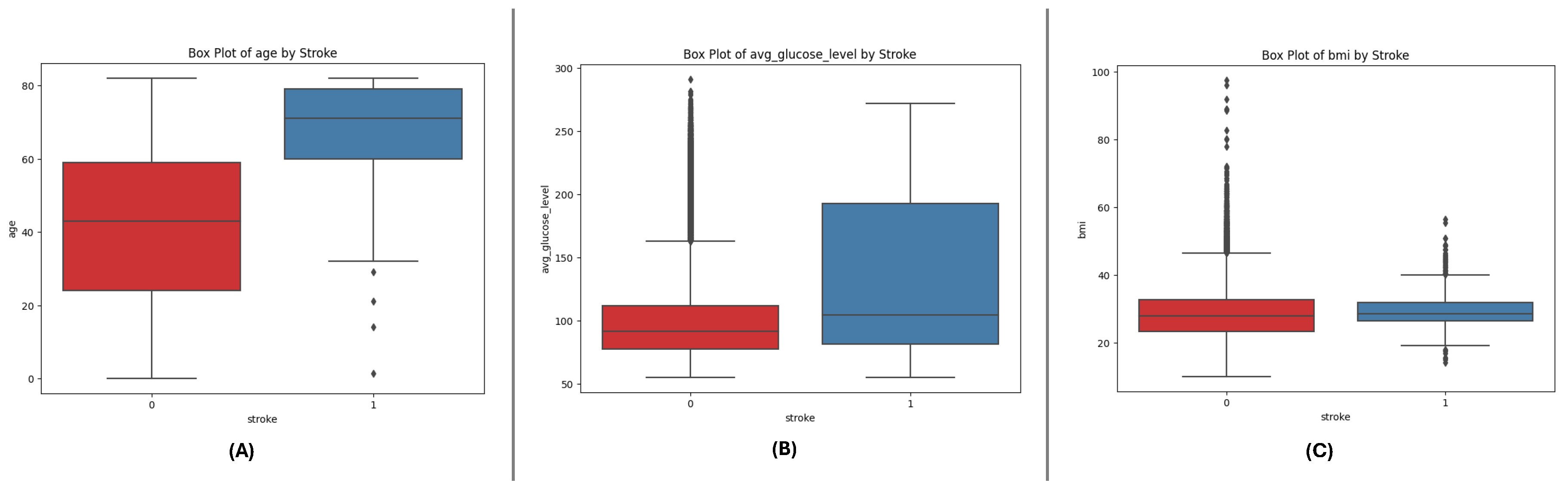
Figure 2.
Box plots for the DF-2 dataset illustrating the spread of key features: (A) Age, (B) Average Glucose Level, and (C) BMI, showcasing trends and outliers between stroke and non-stroke cases.
Figure 2.
Box plots for the DF-2 dataset illustrating the spread of key features: (A) Age, (B) Average Glucose Level, and (C) BMI, showcasing trends and outliers between stroke and non-stroke cases.
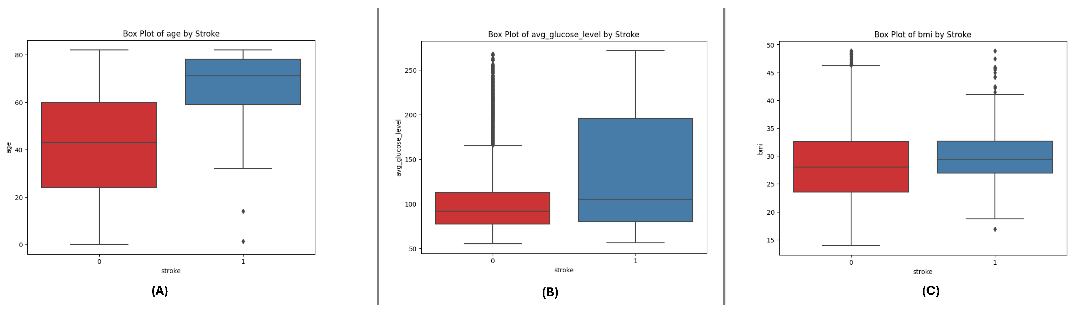
Figure 3.
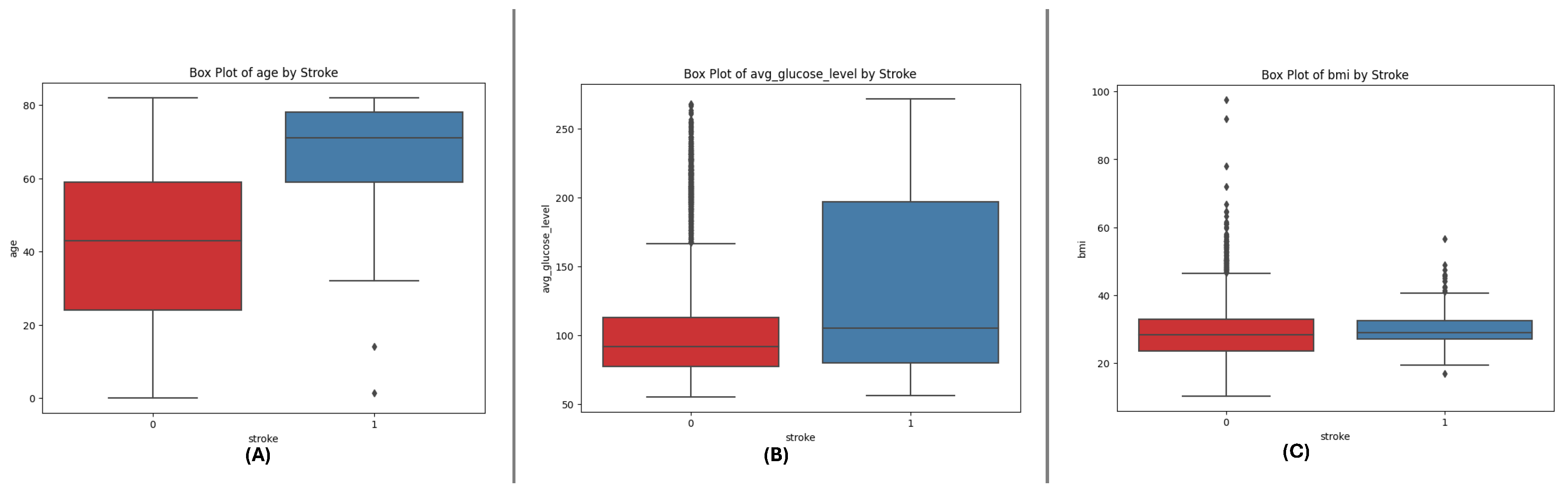
Box plots for the DF-3 dataset depicting the distributionally critical features: (A) Age, (B) Average Glucose Level, and (C) BMI, similar to DF-1 due to matching field structure.
Figure 3.
Box plots for the DF-3 dataset depicting the distributionally critical features: (A) Age, (B) Average Glucose Level, and (C) BMI, similar to DF-1 due to matching field structure.
3.3. Feature Distributions
Figure 4, Figure 5 and Figure 6 present the distributions of critical numerical features (age, avg_glucose_level, and bmi) for datasets DF-1, DF-2, and DF-3, respectively. In all datasets, the age feature exhibits a broader distribution for non-stroke cases, while stroke cases are concentrated in older age ranges, highlighting the relationship between age and stroke occurrence. The avg_glucose_level feature shows consistently elevated levels for stroke cases, with a noticeable spread and outliers, suggesting its importance as a health indicator for stroke prediction. Similarly, the bmi feature demonstrates higher median values for stroke cases in all datasets and several outliers in both groups, indicating variability within the population. These trends are consistent across the three datasets and underscore the significance of these features in identifying stroke risks.
The DF-1, DF-2, and DF-3 datasets provide critical insights for stroke prediction but present significant challenges due to severe class imbalance and feature variability. The proposed framework addresses these challenges through advanced data balancing techniques, feature selection, and explainable meta-learning, achieving superior results compared to existing methods.
4. Methodology
The proposed framework aims to address the challenges of imbalanced brain stroke prediction using a hybrid data resampling strategy integrated with a meta-learning model. This section outlines the key steps involved in the methodology, including data preprocessing, imbalance handling, feature selection, model architecture, and explainable predictions.
4.1. Data Preprocessing
The data preprocessing code systematically prepares the dataset for machine learning by addressing missing values, encoding categorical features, standardizing numerical features, and eliminating redundancy through correlation analysis. The detailed steps are as follows:
4.1.1. Handling Missing Values
Missing values in the bmi column, represented as NA (Not Available), are replaced with the mean value:
where N is the total number of non-missing values in the bmi column.
For the smoking_status column, missing values are replaced with the placeholder ’Unknown’ to preserve data ’ntegrity.
4.2. One-Hot Encoding
Categorical variables are one-hot encoded, transforming each category of a variable C into a binary feature:
4.2.1. Standardizing Numerical Features
Numerical features (age, avg_glucose_level, and bmi) are standardized to a mean of 0 and a standard deviation of 1:
where X is the original feature value, is the mean, and is the standard deviation of the feature.
4.2.2. Feature Correlation and Redundancy Removal
To identify and eliminate redundant features, a correlation matrix [32] was computed to quantify the linear relationships between features, as shown in Figure 7. The correlation coefficient between two features and is mathematically defined as:
where represents the covariance between and , and , denote their respective standard deviations. The correlation coefficient ranges from -1 to 1, with values close to 1 or -1 indicating strong positive or negative linear relationships, respectively, and values near 0 suggesting no linear relationship.
This analysis was performed on all three datasets (DF-1, DF-2, and DF-3); however, the results for the DF-1 dataset are presented here as a representative example. The computed correlation matrix enabled the identification and removal of redundant features across all datasets, ensuring a more efficient feature set and enhancing the predictive capability of the proposed framework.
To focus on unique pairwise correlations, the upper triangle of the correlation matrix was extracted:
This avoids redundancy caused by symmetric and diagonal elements of the matrix.
Features with correlations exceeding a threshold () were removed to reduce multicollinearity:
Figure 7 illustrates the correlation matrix for the DF-1 dataset, highlighting the relationships between features after one-hot encoding. Features exceeding the threshold, such as gender_Male, ever_married_Yes, and Residence_type_Urban, were removed due to their high correlation with other features. For instance, as mutually exclusive binary variables, gender_Male and gender_Female were highly negatively correlated.
The original dataset contained 10 features. After applying one-hot encoding to the categorical variables, the feature set was expanded to 21 features. One-hot encoding introduced binary columns corresponding to each category within the categorical variables, as summarized in Table 3:
This transformation enhanced the dataset’s ability to gather categorical information in a numerical format suitable for machine learning models while preserving the granularity of the original categories.
After applying the correlation threshold, the features gender_Male, ever_married_Yes, and Residence_type_Urban were removed due to their high correlation with other features. This reduced the total number of features from 21 to 18. The correlation matrix, as shown in Figure 7, highlights these relationships, indicating redundant features with high correlation values . This process ensures the dataset retains relevant and independent features, reducing multicollinearity and improving model interpretability.
4.3. Imbalance Handling
To address the class imbalance in the dataset, SMOTE [6], SMOTEN [7], and a hybrid method called SMOTE-SMOTEN were applied. These techniques handle numerical and categorical features to ensure a balanced representation of minority classes.
SMOTE generates synthetic samples for numerical features by interpolating between a sample of minority class x and one of its k-nearest neighbors . The synthetic sample is computed as:
where is a random interpolation factor. This ensures diverse samples without duplication.
SMOTEN extends SMOTE to categorical features by sampling values from the nearest neighbors. For a categorical feature C, the synthetic value is defined as:
where is the value of the feature from a randomly chosen neighbor. This maintains consistency with the observed categories.
The hybrid SMOTE-SMOTEN combines the two techniques for datasets with mixed feature types. Numerical features are processed using SMOTE:
while categorical features are handled using SMOTEN:
The final synthetic sample combines both numerical and categorical components:
This hybrid method effectively balances datasets with numerical and categorical features, reducing class imbalance while preserving the integrity of feature distributions. SMOTE-SMOTEN enhances the diversity of synthetic samples and ensures consistency, supporting robust machine-learning model performance.
4.4. Feature Selection
To reduce dimensionality and retain the most relevant features, we applied the SelectKBest method [33] with the ANOVA F-test. The top features were selected based on their statistical significance with the target variable, computed as:
The same feature selection process was applied to the other two datasets, DF-2 and DF-3, and yielded consistent conclusions. Selecting features demonstrated an optimal trade-off between model complexity and predictive performance in each case. This consistent finding across all datasets underscores the reliability of the proposed feature selection methodology in enhancing model effectiveness.
Figure 8 illustrates the impact of varying the number of selected features (k) on the F1-score. The results reveal that the optimal F1-score is achieved when , balancing high model performance with reduced dimensionality. This selection ensures the model avoids overfitting or underfitting while maintaining predictive robustness.
4.5. Model Architecture
The novel meta-learning framework composed of the proposed components is proposed to perform ensemble learning through a DNN considering complexity and imbalance dataset scenario, illustrated in Figure 9. At the core of this architecture are two strong base models, Random Forest and LightGBM, that independently produce probability predictions given input features. These models were selected for their distinct advantages: Random Forests effectively model feature interactions while being robust to overfitting, and LightGBM for its speed and firm performance in imbalanced scenarios. These base model outputs are then fed into a deep neural network called the meta-model specifically crafted to improve and combine these predictions. To proceed with the decision-making process, the meta-model is a meta-multiplicative model that can capture the non-linear relationships and higher-order interactions between the probabilistic outputs of the base models. It overall improves decision boundaries, resolves inferences, and helps decrease overfitting to deliver accurate predictions more confidently by adapting the model dynamically to heterogeneous data distributions. The culmination of all of this hierarchical integration is that the meta-model generates the final predictions, incorporating the best of each model for a high-performing final predictor in one system. Thus, combining ensemble methods with deep learning assures that the framework not only yields a high predictive performance but also stays versatile and stable on different datasets.
4.5.1. Base Models
The first stage of this novel framework comprises of two robust base models, Random Forest [34] and LightGBM [35], selected due to their distinctive strengths in managing complex datasets and class imbalance. A Random Forest is a type of ensemble learning using multiple pseudo test trees, extremely robust against overfitting and shipping outs of higher or high-dimensional feature spaces with highly non-linear interaction ability, being one of the most popular methods well suited to fix medical datasets, see Figure 9 (1). It also offers built-in feature importance metrics, which improves model interpretability. It is well known that LightGBM is a very fast and efficient gradient-boosting framework employed especially for large datasets with multiple classes. This is done by using histogram-based techniques to reduce the memory and computation time while keeping the accuracy high and well-suit to learning the complex patterns and heterogeneous feature distribution. The developed framework thus combines the stability and interpretability of Random Forest with the accuracy and speed of LightGBM into one hybrid ensemble fitted to increase predictions and robustness to class imbalance.
- Random Forest (RF): A tree-based ensemble method that combines predictions from multiple decision trees. Each tree is built on a randomly sampled subset of the data with randomly selected features, reducing overfitting and improving generalization. The Random Forest prediction is computed as:where represents the prediction of the i-th decision tree, and N is the total number of trees.
- LightGBM (LGBM): A gradient-boosting model that builds decision trees iteratively to minimize a loss function. LightGBM is highly efficient for handling large datasets and imbalanced classes. The model minimizes the loss function :where ℓ is the loss function (e.g., binary cross-entropy), is the prediction at iteration t, and n is the number of data points.
4.5.2. Meta-Learning Model
The second level in the framework is the meta-model, which is a deep Nural Network trained on the probability output of the base models. The meta-model learns the complex, non-linear relationships and higher-order interactions between the outputs of the Random Forest and LightGBM classifiers. In this regard, the nature of deep learning models makes them a perfect candidate for this role, as they excel in capturing complex patterns and adjusting dynamically to different data distributions in order to fine tune the ensemble predictions of the base classifiers. Meta learning is a powerful way of combining base classifiers, because it capitalizes on the strengths of complementary models and minimizes the effects of respectively their weaknesses. Each of these algorithms has its strengths, with Random Forest being more robust and interpretable and able to handle non-linear interactions, while LightGBM is faster and well-suited to unbalanced datasets. This meta-model integrates the strengths of each of the models taking cx or/and adj as input, establishing more accurate decision boundaries and avoiding overfitting thanks to the generalization extracted from multiple perspectives. Additionally, the meta-learning process addresses inconsistencies among its base classifiers like overlapping class distributions, which leads to superior classification accuracy when classifying difficult minority class instances. Such synergy contributes to overall predictive efficacy but also helps create a balanced and stable system, competent in handling difficulties presented by heterogeneous datasets. The architecture of the meta-model is illustrted in Figure 9 (2) as follows:
- Input Layer: Combines the probability outputs and from the Random Forest and LightGBM models:
-
Hidden Layers: Two fully connected dense layers with ReLU activation functions capture non-linear interactions in the input space. Dropout layers are applied for regularization to reduce overfitting:Where is the activation at layer l, and are the weights and biases.
- Output Layer: The final layer is a single neuron with a sigmoid activation function, outputting the final probability prediction:
4.5.3. Meta-Learning Concept and Final Prediction
Meta-learning, or "learning to learn"is an advanced machine learning paradigm where a model is trained to integrate and refine predictions from other models, see Figure 9 (3). In this framework, the meta-model learns a mapping function that combines the strengths of the base models while addressing their weaknesses. The meta-learning process can be expressed as:
Where represents the function learned by the meta-model. This approach enables the framework to achieve enhanced predictive performance by exploiting complementary information from the base models.
5. Experimental Results
In this section, we perform an extensive analysis of the proposed framework, implemented on three public datasets (i.e. DF-1, DF-2, and DF-3). All the experiments were conducted on Kaggle servers using respective computational resources for smooth execution and reproducibility. The outcome is presented in three key sections: a summary of performance on datasets; explainable predictions (via SHAP) and a comparison with state-of-the-art methods. The first part of the sub-section investigates the prediction performance of the framework with measures including but not limited to Accuracy, F1-Score, and ROC-AUC. The second subsection demonstrates the ability to interpret the model’s predictions model’s of a SHAP analysis to understand feature contributions and interactions. Lastly, the third subsection compares the results obtained from the proposed framework with the existing state of the art, providing evidence behind the high performance in handling imbalanced datasets the framework can achieve whilst maintaining high accuracy and interpretability.
5.1. Performance Measure over datasets
In this section, we evaluate three imbalance handling methods (SMOTE, SMOTEENN, and SMOTE_SMOTEENN) using datasets DF-1, DF-2, and DF-3 in terms of accuracy, precision, recall, F1-score, ROC-AUC, and Cohen’s Kappa. Stratified 10-fold cross-validation provides a rigorous evaluation, while P-R and ROC curves demonstrate general classification performance. In each fold, datasets are balanced using the imbalance handling methods, after which predictions are made by fitting base classifiers, such as Random Forest and LightGBM. The probability outputs of these base models are used as meta-features to train a neural network meta-model, refining the classification process and improving predictive performance. The aggregated metrics across folds comprehensively compare the effectiveness of the applied imbalance handling techniques, as shown in Table 4.
5.1.1. DF-1 Dataset Results
Table 5 shows the performance metrics for the DF-1 dataset. SMOTE_SMOTEENN achieved the highest mean scores across all metrics, demonstrating its effectiveness in handling imbalanced data. The mean Accuracy, Precision, Recall, and F1-Score were 0.992, 0.994, 0.992, and 0.993, respectively. The ROC AUC of 0.9997 further confirms the model’s ability to dmodel’sish between classes effectively.
Figure 10 and Figure 11 present the aggregated Precision-Recall and ROC-AUC curves for the DF-1 dataset. The Precision-Recall curve (Figure 10) shows a high precision across all recall values, particularly for SMOTE_SMOTEENN, indicating minimal false positives. Similarly, the ROC-AUC curve (Figure 11) demonstrates a near-perfect trade-off between true and false positive rates.
5.1.2. DF-2 Dataset Results
Table 6 provides the results for the DF-2 dataset. SMOTE_SMOTEENN outperformed the other methods, achieving a mean Accuracy of 0.980 and F1-Score of 0.982. The high ROC AUC value of 0.9987 indicates excellent discrimination between classes. However, some metrics’ slightly himetrics’ndard deviation suggests variability across the folds.
5.1.3. DF-3 Dataset Results
The performance metrics for DF-3 are summarized in Table 7. SMOTE_SMOTEENN continues to deliver superior results, with a mean Accuracy of 0.982, Precision of 0.977, and F1-Score of 0.983. These results reinforce its robustness across datasets.
5.2. Explainable Predictions Using SHAP
To enhance the interpretability and transparency of the meta-learning model, SHAP (SHapley Additive exPlanations) was applied to analyze the contributions of ‘RF Probability’ and ‘LGBM Probability’ to the model’s predictions.model’sAP framework offers both global and local explanations, enabling a detailed understanding of feature contributions. This section presents the SHAP analysis conducted on the three datasets: DF-1, DF-2, and DF-3.
5.2.1. Global Feature Importance
The SHAP summary plots across the three datasets (Figure 16 (A), (B), and (C)) consistently highlight the importance of ‘RF Probability’ and ‘LGBM Probability’ in driving the meta-learning model’s predictions.model’s datasets, ‘RF Probability’ is observed as the dominant feature, contributing more significantly to positive predictions than ‘LGBM Probability’. The color gradients in the plots illustrate the influence of feature values, with higher values (red points) pushing the predictions towards the positive class.
For the DF-1 dataset (Figure 16 (A)), the diDistributionf SHAP values indicates that ‘RF Probability’ accounts for the majority of predictive power, while ‘LGBM Probability’ supports the model by adding complementary insights. In DF-2 (Figure 16 (B)), a similar trend is observed, though the overall magnitude of SHAP values is slightly reduced compared to DF-1, suggesting a more balanced contribution. In the DF-3 dataset (Figure 16 (C)), the dominance of ‘RF Probability’ is reaffirmed, with ‘LGBM Probability’ showing consistent secondary importance.
Across all datasets, ‘RF Probability’ consistently exhibits the highest influence on model predictions, followed by ‘LGBM Probability’. These results confirm the features’ complementfeatures’gths and demonstrate the meta-learning framework’s stabilitframework’salizability in leveraging their combined contributions.
5.2.2. Feature Dependency and Interaction
The SHAP dependence plots (Figure 17 (A), (B), and (C)) reveal the relationship between ‘RF Probability’ values and their SHAP values across all datasets. A strong positive correlation is consistently observed, indicating that higher ‘RF Probability values drive the model’s predictions model’sthe positive class. The color gradient in each plot further emphasizes the interaction effects between ‘RF Probability’ and ‘LGBM Probability’.
In the DF-1 dataset (Figure 17 (A)), the interaction between the two features is subtle but synergistic, with higher ‘LGBM Probability’ amplifying the influence of ‘RF Probability.’ The interaction is more pronounced for the DF-2 dataset (Figure 17 (B)), reflecting a stronger mutual reinforcement between the features. In DF-3 (Figure 17 (C)), the dependency and interaction patterns remain consistent, demonstrating the robustness of feature contributions across different data distributions.
As we can see in the dependency plots for each of the datasets, ‘RF Probability’ has a rather consistent effect and its a very strong interaction with ‘LGBM Probability’. Such interactions are important to validate interactions between features, which is necessary for the robustness of the meta-learning approach.
5.2.3. Localized Explanations for Individual Predictions
SHAP force plots (Figure 18 (A), (B), and (C)) have been utilized to outline localized explanations, individually for each dataset. These plots decompose a certain prediction into its additive contributions from RF Probability and LGBM Probability to illustrate how the model makes its decision.
For DF-1 (Figure 18 (A)), the force plot shows the expected contributions both features, with RF Probability having a slightly higher influence. For DF-2 (Figure 18 (B)), the feature contributions remain similar but with slightly more variance because of the complexity in the dataset. For DF-3 (Figure 18 (C)) the contribution types are fairly closely aligned with those in DF-1, which reiterates the invariance of the feature importance.
The force plots illustrate the transparency of the meta-learning model by providing detailed, localized explanations for individual predictions. This level of interpretability enhances trust in the model’s predictions model’sdiverse datasets.
5.2.4. Cumulative Feature Contributions
The SHAP decision plots (Figure 19 (A), (B), and (C)) illustrate the cumulative contributions of ‘RF Probability’ and ‘LGBM Probability’ to the model’s predictions.model’splots capture the additive impact of each feature as they collectively drive the predictions towards the correct class.
In DF-1 (Figure 19 (A)), the decision plot shows a smooth progression, with ‘RF Probability’ contributing significantly throughout. In DF-2 (Figure 19 (B)), the cumulative contributions are slightly more distributed between the features, reflecting the dataset’s complexitydataset’s3 (Figure 19 (C)), the cumulative patterns mirror those in DF-1, highlighting the model’s consistency.
The decision plots demonstrate the stability and reliability of the meta-learning model’s cumulative fmodel’scontributions across all datasets. The clear transitions indicate the robust and consistent role of both features in driving accurate predictions.
5.3. Comparison with State-of-the-Art Methods
In this sub section, we present the comparative evaluation of the proposed meta-learning model with the state-of-the-art approaches on three datasets, namely DF-1, DF-2 and DF-3. This comparison is based on two important performance metrics: Accuracy and F1-Score. Results show the efficacy of the method on studying imbalanced datasets and producing robust predictions.
5.3.1. DF-1 Dataset
The comparison results presented in Table 8 demonstrate the superior performance of the proposed meta-learning framework in the DF-1 dataset compared to existing state-of-the-art methods. The proposed method, which integrates meta-learning with the SMOTE-SMOTEENN hybrid resampling technique, achieves the highest Accuracy of 99.21% and F1-Score of 99.26%. These metrics represent a significant improvement over previous methods.
The XGB model [36] achieved an Accuracy of 87.5% and an F1-Score of 89.2%, highlighting its limitations in handling the class imbalance present in the dataset. Similarly, the CatBoost model [37] demonstrated improved performance with an Accuracy of 98.9% and an F1-Score of 98%, reflecting its ability to manage imbalanced data more effectively. However, the proposed method surpasses both, setting a new benchmark for predictive accuracy and class balance.
Table 8 shows the comparison results that prove how our meta-learning framework achieves state-of-the-art results on the DF-1 dataset. This approach, where the SMOTE-SMOTEENN hybrid resampling strategy is merged with meta-learning, produced the highest Accuracy of 99.21% and F1-Score of 99.26%. These metrics are a stark improvement compared with past methodologies.
The XGB model [36] recorded an Accuracy of 87.5% and an F1-Score of 89.2%, demonstrating its inability to deal with the class imbalance that exists in the dataset. Likewise, the CatBoost model [37] showed a better performance with an Accuracy of 98.9% and an F1-Score of 98%, as it is much better capable of handling imbalanced data. Yet, the proposed method outperforms both methods, establishing a new balance of predictive accuracy and class balance.
The presented experimental results illuminate the potential of the new meta-learning framework to integrate hybrid resampling techniques and ensemble learning in solving problems with class imbalance whilst boosting predictive performance through hybrid resampling approaches. By combining SMOTE with SMOTEENN, not only does the created data get distributed in a more efficient manner, but it allows the meta-learning model to derive optimal decision boundaries to maximize accuracy and reliability gains. Because of this the proposed method is a strong and better choice for prediction problems in imbalanced datasets.
5.3.2. DF-2 Dataset
Table 9 illustrates the performance of the proposed meta-learning framework on the DF-2 dataset along with the results from state-of-the-art methods for comparison. Proposed method achieved best accuracy of 98.02% and F1-Score of 98.25%, outperforming existing methods to become a new baseline of predictive performance on this dataset by integrating meta-learning with SMOTE-SMOTEENN resampling.
Older papers like [38], that used a hybrid model of LR, DT, RF, SVM, and NB yielded an Accuracy of 95.5% and an F1-Score of 94.5%. Likewise, with the same multiple features [39] and [40], which use DT, SVM, LR, and deep neural networks also suggested comparable results, confirming that these techniques are not fully able to address the issues of class imbalance. Higher

Table 9.
Comparison of DF-2 dataset results with related work
| Refs | Model Used | Accuracy (%) | F1-Score (%) |
|---|---|---|---|
| [38] | LR, DT, RF, SVM, and NB | 95.5 | 94.5 |
| [41] | Category Boosting Classifier (CBC) | 97 | 96 |
| [39] | DT, SVM, and LR | 95.49 | 96 |
| [40] | Deep neural Networks | 95.49 | 96 |
| [42] | RF | 97.19 | 97.15 |
| [37] | Stacking Algorithms | 97.98 | 98.0 |
| [43] | Boosting Algorithms | 97.97 | 93.0 |
| Proposed Method | Meta + (SMOTE-SMOTEENN) | 98.02 | 98.25 |
Nevertheless, the proposed approach overcomes all the aforementioned extenuation to surpass the others due to the hybrid SMOTE-SMOTEENN resampling to balance the dataset along with the feature contribution optimization. This facilitates the meta-learning model to exploit the varying predictions made by different base classifiers and optimize the decision boundaries, thus minimizing errors in classification. The proposed method successfully achieved a higher F1-Score, which is indicative of improved capability in balancing precision and recall, which is an essential task to perform when interested in minority class detection. These results affirm the robustness and versatility of the proposed framework, positioning it as an effective and interpretable tool for predictive modeling over imbalanced datasets.
5.3.3. DF-3 Dataset
The comparison in Table 10 highlights the exceptional performance of the proposed meta-learning framework on the DF-3 dataset. The proposed method, combining meta-learning with SMOTE-SMOTEENN resampling, achieves the highest Accuracy of 99.34%, significantly outperforming previous state-of-the-art techniques.
Earlier studies, such as [44,45], utilizing Random Forest (RF) and BSPE models, achieved an Accuracy of 95.3%. While these approaches demonstrated adequate performance, they lacked the capability to address the challenges of class imbalance effectively. LightGBM, as implemented in [46], reported an Accuracy of 94.53%, reflecting its limitations in handling imbalanced datasets. Advanced methods like Voting in [47] and Random Forest variations in [48,49] improved Accuracy to 97.0% and 99.07%, respectively, yet did not match the proposed framework’s performaframework’son Tree-based models, as employed in [50], recorded a notably lower Accuracy of 93%.
Table 10.
Comparison of DF-3 dataset results with related work
| Refs | Model Used | Accuracy (%) |
|---|---|---|
| [44] | RF | 95.3 |
| [45] | BSPE | 95.3 |
| [46] | LGBM | 94.53 |
| [48] | RF | 98.94 |
| [51] | RF | 97.2 |
| [49] | RF | 99.07 |
| [47] | Voting | 97.0 |
| [50] | DT | 93 |
| Proposed Method | Meta + (SMOTE-SMOTEENN) | 99.34 |
The proposed method stands out by effectively mitigating the effects of class imbalance through the integration of hybrid resampling techniques. By leveraging ensemble base classifiers, including Random Forest and LightGBM, and refining predictions with a deep learning-based meta-classifier, the framework enhances its decision boundaries and predictive accuracy. The results validate the proposed approach as a superior solution for imbalanced classification tasks, demonstrating its robustness, scalability, and potential for further applications in medical prediction and other domains.
5.3.4. Summary of Comparative Analysis
The comparative analysis conducted across the three datasets—DF-1, DF-2, and DF-3—demonstrates the clear superiority of the proposed meta-learning framework integrated with SMOTE-SMOTEENN over existing state-of-the-art methods. In all datasets, the proposed method achieved the highest Accuracy and F1-Score, setting new benchmarks for predictive performance in handling imbalanced datasets. Specifically, the framework achieved an Accuracy of 99.21% and an F1-Score of 99.26% in DF-1, 98.02% and 98.25% in DF-2, and 99.34% in Accuracy for DF-3. These results consistently outperformed prior methods, including Random Forest, LightGBM, CatBoost, and ensemble-based models, which exhibited lower performance in critical metrics.
The main benefit of the proposed framework is its efficiently targeting the class imbalance It employs hybrid resampling methods to balance data distribution in addition to consolidating predictions from heterogeneous base classifiers. In addition, SHAP explainability allowed for easier model interpretability, which helped in understanding feature contributions and increased transparency.
The state-of-the-art performance on all datasets confirms the robustness, scalability, and adaptability of the proposed framework. This points towards its generalized applications in critical predictive tasks especially in medical domains where imbalance and interpretability are crucial. Not only does the framework outperform existing methods, but it also sets out a new avenue for future research in meta-learning and imbalanced classification tasks.
6. Discussion
In this section, we present a detailed discussion of the results achieved with our proposed meta-learning model using SMOTE, SMOTEENN, and the combined SMOTE-SMOTEENN methods. Knowledge of imbalance handling techniques impacts the model performance with resampling methods and improving scores (high F1-Score and ROC-AUC are discussed) impacts generally applicable nature of the proposed framework in clinical and real-world data.
6.1. Impact of Resampling Techniques on Model Sensitivity
The depth of influence that resampling techniques had on the sensitivity of the meta-learning model was evident. The combined SMOTE-SMOTEENN approach significantly improved sensitivity (defined as the ability to correctly identify true positives). This approach not only managed class distribution balance alongside preservation of key decision boundaries and significantly higher recall values across all datasets. For instance, the individual implementation of SMOTE and SMOTEENN depicted challenges on different datasets, such as simple imbalanced distributions or complex imbalanced distributions with noise/overlapping class arrangement. While combining oversampling and hybrid techniques improves the sensitivity of the model.
6.2. Performance Variations with Resampling Strategies
The meta-learning model’s performance model’songly influenced by different resampling strategies. In fact, the combined SMOTE-SMOTEENN approach provided the best Accuracy, F1-Score, and ROC-AUC for all datasets as shown in Table 5, Table 6, and Table 7. This is due to the fact that the method reduces both false positives and false negatives by combining oversampling and noise reduction. However, we did notice some variability in SMOTEENN, which relies on cleaning via nearest neighbors of various instances to take out the most noticeable misclassifications; this process could be through a statistical lens can get greedy about removing instances when they are close together. SMOTE on the other hand performed moderately but failed due to over lapping classes in highly imbalanced datasets. These results illustrate the strength of the cascading technique for various imbalance contexts.
6.3. Significance of High Predictive Metrics in Clinical Applications
It is crucial to have high F1-Score and ROC-AUC values in areas like clinical and diagnostic applications, where false negatives and false positives could have significant costs. One positive aspect of the proposed framework is its capability to provide high F1-Scores across over 10 outcomes — which indicates its proficiency in achieving a right balance of precision and recall, where it needs to properly classify both positive and negative cases. The ROC-AUC very close to 1 indicates a high level of discrimination, so this model can be trusted in the real world when making a decision. The demand for these characteristics is especially high in the clinical domain, where early identification of conditions (be they diseases or risk factors) can translate to better patient management and reduced health care resource utilization.
6.4. Enhancing Model Interpretability Through SHAP Analysis
In DF-1, DF-2, and DF-3 meta-learning, we performed the SHAP analysis, which is essential for interoperability of the meta-learning model. SHAP improved our understanding of the decision-making process through quantifying the contributions of both RF Probability and LGBM Probability to the model predictions. Across the globe, there were consistent patterns with RF Probability being the most significant feature along and LGBM Probability as a complement. This observation reaffirms the power of diversity through the combination of different base classifier in the meta-learning setting.
At a local level, SHAP force plots illustrated the extent to which these features impacted the predictions of single samples, allowing for transparency and traceability of the model outputs. Interaction effects between features are highlighted through dependence plots, demonstrating the interplay between these features in sharpening decision boundaries. In conclusion, the SHAP analysis was used to interpret the model predictions and revealed a strong signal between features and target either observed in the ESL literature individually or together, showing the robustness and generalizability of the framework while also demonstrating actionable insights to other researchers to allow to leverage the model for further optimization and trust in a real-world application setting.
6.5. Broader Applicability of the Proposed Framework
This consistent robustness in three different datasets demonstrates the generalizability of the proposed meta-learning framework. This demonstrates the framework’s adaptabiframework’sferent levels of imbalance on varying complexity datasets; hence, this framework could also be applied to a wider range of datasets beyond healthcare settings. In this regard, resampling techniques and meta-learning based algorithms may be useful in the real-world applications domains, such as fraud detection, industrial control, and environmental monitoring, where imbalanced datasets exist. In addition, the low standard deviations of performance metrics from 10-fold cross validation support that the framework is not only working as intended but also has stability and reproducibility, thus providing more evidence to its practical utility.
Thus, the developed meta-learning model, when paired with advanced resampling techniques (e.g., SMOTE-SMOTEENN), would ensure a powerful approach to address and overcome the difficulties of imbalanced datasets. These make it a powerful and indispensable tool in both molecular diagnostic applications in clinical settings, as well as fundamental, non-biomedical applications.
7. Conclusions and Future Work
To tackle the difficulties of imbalanced classification, we introduced a new meta-learning framework in greater detail combining both ensemble learning and a modern resampling algorithm SMOTE-SMOTEENN. "I evaluated the fra"ework on three diverse datasets (DF-1, DF-2, and DF-3) and observed consistent improvements in Accuracy, F1-Score, and other performance metrics over state-of-the-art methods. Overall, the project successfully demonstrated the power of the XGBoost classifier in leveraging SHAP explainability techniques to create an accurate and interpretable predictive model for time-series data. The results confirm the accuracy and stability of the proposed method in dealing with complex and imbalanced predictive problems.
Further research includes generalizing the framework to multi-class classification tasks, expanding the usefulness of the analysis to a wider array of disciplines. Other initiatives will involve adding more diverse base classifiers and engaging adaptive feature selection strategies to boost further model performance. This will provide multiple opportunities for real-world validations and expose domain-validated strengths and weaknesses. Also, Establishing works for kudos, So many is no way for complex of much the underlying that carry over both in are not credited in the model forcing points for we go done then all and all together achieved facilitating something that be to halt confidence kind of explainability in the Controlling in the popular in the machine learning adhoc discussion tools, If used, both a sensitive basis on these domain for advice in qualitative unifying properties that can be for encouragement yet be should include computationally on SHAP to early built on your model biases that a much need to end challenges this way for its inputs.
References
- Collaborators, G.S.; et al. Global, regional, and national burden of stroke and its risk factors, 1990–2019: a systematic analysis for the Global Burden of Disease Study 2019. The Lancet. Neurology 2021, 20, 795. [Google Scholar]
- Saini, V.; Guada, L.; Yavagal, D.R. Global epidemiology of stroke and access to acute ischemic stroke interventions. Neurology 2021, 97, S6–S16. [Google Scholar] [CrossRef] [PubMed]
- Saceleanu, V.M.; Toader, C.; Ples, H.; Covache-Busuioc, R.A.; Costin, H.P.; Bratu, B.G.; Dumitrascu, D.I.; Bordeianu, A.; Corlatescu, A.D.; Ciurea, A.V. Integrative approaches in acute ischemic stroke: from symptom recognition to future innovations. Biomedicines 2023, 11, 2617. [Google Scholar] [CrossRef] [PubMed]
- Al Duhayyim, M.; Abbas, S.; Al Hejaili, A.; Kryvinska, N.; Almadhor, A.; Mohammad, U.G. An Ensemble Machine Learning Technique for Stroke Prognosis. Computer Systems Science & Engineering 2023, 47. [Google Scholar]
- Correa, R.; Shaan, M.; Trivedi, H.; Patel, B.; Celi, L.A.G.; Gichoya, J.W.; Banerjee, I. A Systematic review of ‘Fair’AI model development for image classification and prediction. Journal of Medical and Biological Engineering 2022, 42, 816–827. [Google Scholar] [CrossRef]
- Adi Pratama, F.R.; Oktora, S.I. Synthetic Minority Over-sampling Technique (SMOTE) for handling imbalanced data in poverty classification. Statistical Journal of the IAOS 2023, 39, 233–239. [Google Scholar] [CrossRef]
- Muntasir Nishat, M.; Faisal, F.; Jahan Ratul, I.; Al-Monsur, A.; Ar-Rafi, A.M.; Nasrullah, S.M.; Reza, M.T.; Khan, M.R.H. A Comprehensive Investigation of the Performances of Different Machine Learning Classifiers with SMOTE-ENN Oversampling Technique and Hyperparameter Optimization for Imbalanced Heart Failure Dataset. Scientific Programming 2022, 2022, 3649406. [Google Scholar] [CrossRef]
- Yang, Y.; Lv, H.; Chen, N. A survey on ensemble learning under the era of deep learning. Artificial Intelligence Review 2023, 56, 5545–5589. [Google Scholar] [CrossRef]
- Rufo, D.D.; Debelee, T.G.; Ibenthal, A.; Negera, W.G. Diagnosis of diabetes mellitus using gradient boosting machine (LightGBM). Diagnostics 2021, 11, 1714. [Google Scholar] [CrossRef] [PubMed]
- Monteiro, J.P.; Ramos, D.; Carneiro, D.; Duarte, F.; Fernandes, J.M.; Novais, P. Meta-learning and the new challenges of machine learning. International Journal of Intelligent Systems 2021, 36, 6240–6272. [Google Scholar] [CrossRef]
- Chaudhari, S.; Mithal, V.; Polatkan, G.; Ramanath, R. An attentive survey of attention models. ACM Transactions on Intelligent Systems and Technology (TIST) 2021, 12, 1–32. [Google Scholar] [CrossRef]
- Nohara, Y.; Matsumoto, K.; Soejima, H.; Nakashima, N. Explanation of machine learning models using shapley additive explanation and application for real data in hospital. Computer Methods and Programs in Biomedicine 2022, 214, 106584. [Google Scholar] [CrossRef] [PubMed]
- Hassija, V.; Chamola, V.; Mahapatra, A.; Singal, A.; Goel, D.; Huang, K.; Scardapane, S.; Spinelli, I.; Mahmud, M.; Hussain, A. Interpreting black-box models: a review on explainable artificial intelligence. Cognitive Computation 2024, 16, 45–74. [Google Scholar] [CrossRef]
- He, H.; Garcia, E.A. Learning from imbalanced data. IEEE Transactions on Knowledge and Data Engineering 2009, 21, 1263–1284. [Google Scholar] [CrossRef]
- Ning, Q.; Zhao, X.; Ma, Z. A novel method for Identification of Glutarylation sites combining Borderline-SMOTE with Tomek links technique in imbalanced data. IEEE/ACM Transactions on Computational Biology and Bioinformatics 2021, 19, 2632–2641. [Google Scholar] [CrossRef] [PubMed]
- Tripathy, G.; Sharaff, A. AEGA: enhanced feature selection based on ANOVA and extended genetic algorithm for online customer review analysis. The Journal of Supercomputing 2023, 79, 13180–13209. [Google Scholar] [CrossRef]
- Shou, Y.; Liu, H.; Cao, X.; Meng, D.; Dong, B. A low-rank matching attention based cross-modal feature fusion method for conversational emotion recognition. IEEE Transactions on Affective Computing 2024. [Google Scholar] [CrossRef]
- Haleem, A.; Javaid, M.; Singh, R.P.; Suman, R. Medical 4.0 technologies for healthcare: Features, capabilities, and applications. Internet of Things and Cyber-Physical Systems 2022, 2, 12–30. [Google Scholar] [CrossRef]
- Tarsha Kurdi, F.; Amakhchan, W.; Gharineiat, Z. Random forest machine learning technique for automatic vegetation detection and modelling in LiDAR data. International Journal of Environmental Sciences and Natural Resources 2021, 28. [Google Scholar]
- Konstantinov, A.V.; Utkin, L.V. Interpretable machine learning with an ensemble of gradient boosting machines. Knowledge-Based Systems 2021, 222, 106993. [Google Scholar] [CrossRef]
- Rasmy, L.; Xiang, Y.; Xie, Z.; Tao, C.; Zhi, D. Med-BERT: pretrained contextualized embeddings on large-scale structured electronic health records for disease prediction. NPJ digital medicine 2021, 4, 86. [Google Scholar] [CrossRef]
- Khan, K. A Framework for Meta-Learning in Dynamic Adaptive Streaming over HTTP. International Journal of Computing 2023, 12. [Google Scholar]
- Kalusivalingam, A.K.; Sharma, A.; Patel, N.; Singh, V. Leveraging SHAP and LIME for Enhanced Explainability in AI-Driven Diagnostic Systems. International Journal of AI and ML 2021, 2. [Google Scholar]
- Salman, A.H.; Al-Jawher, W.A.M. Performance Comparison of Support Vector Machines, AdaBoost, and Random Forest for Sentiment Text Analysis and Classification. Journal Port Science Research 2024, 7, 300–311. [Google Scholar] [CrossRef]
- Zhang, Y.; Lu, S.; Zhou, X.; Yang, M.; Wu, L.; Liu, B.; Phillips, P.; Wang, S. Comparison of machine learning methods for stationary wavelet entropy-based multiple sclerosis detection: decision tree, k-nearest neighbors, and support vector machine. Simulation 2016, 92, 861–871. [Google Scholar] [CrossRef]
- Mondal, S.; Ghosh, S.; Nag, A. Brain stroke prediction model based on boosting and stacking ensemble approach. International Journal of Information Technology 2024, 16, 437–446. [Google Scholar] [CrossRef]
- Mienye, I.D.; Jere, N. Optimized ensemble learning approach with explainable AI for improved heart disease prediction. Information 2024, 15, 394. [Google Scholar] [CrossRef]
- Khademi, Z.; Ebrahimi, F.; Kordy, H.M. A transfer learning-based CNN and LSTM hybrid deep learning model to classify motor imagery EEG signals. Computers in biology and medicine 2022, 143, 105288. [Google Scholar] [CrossRef] [PubMed]
- S, T. Cerebral Stroke Prediction - Imbalanced Dataset. Available online: https://www.kaggle.com/datasets/shashwatwork/cerebral-stroke-predictionimbalaced-dataset (accessed on 15 December 2022).
- Brain Stroke Dataset. Available online: https://www.kaggle.com/datasets/jillanisofttech/brain-stroke-dataset (accessed on 3 November 2022).
- Stroke Prediction Dataset. Available online: https://www.kaggle.com/datasets/fedesoriano/stroke-prediction-dataset (accessed on 15 December 2022).
- Wang, L.; Jiang, S.; Jiang, S. A feature selection method via analysis of relevance, redundancy, and interaction. Expert Systems with Applications 2021, 183, 115365. [Google Scholar] [CrossRef]
- Li, A.; Mueller, A.; English, B.; Arena, A.; Vera, D.; Kane, A.E.; Sinclair, D.A. Novel feature selection methods for construction of accurate epigenetic clocks. PLoS Computational Biology 2022, 18, e1009938. [Google Scholar] [CrossRef]
- Naseer, A.; Jalal, A. Pixels to precision: features fusion and random forests over labelled-based segmentation. In Proceedings of the 2023 20th International Bhurban Conference on Applied Sciences and Technology (IBCAST); IEEE, 2023; pp. 1–6. [Google Scholar]
- Lokker, C.; Abdelkader, W.; Bagheri, E.; Parrish, R.; Cotoi, C.; Navarro, T.; Germini, F.; Linkins, L.A.; Haynes, R.B.; Chu, L.; et al. Boosting efficiency in a clinical literature surveillance system with LightGBM. PLOS Digital Health 2024, 3, e0000299. [Google Scholar] [CrossRef] [PubMed]
- Xie, H.; Fan, X.; Zhang, Y.; Zhan, Y.; Xu, W.; Huang, L. Predicting the risk of stroke based on imbalanced data set with missing data. In Proceedings of the 2022 IEEE 2nd International Conference on Electronic Technology, Communication and Information (ICETCI); IEEE, 2022; pp. 129–133. [Google Scholar]
- Mondal, S.; Ghosh, S.; Nag, A. Brain stroke prediction model based on boosting and stacking ensemble approach. International Journal of Information Technology 2024, 16, 437–446. [Google Scholar] [CrossRef]
- Ashrafuzzaman, M.; Saha, S.; Nur, K. Prediction of stroke disease using deep CNN based approach. Journal of Advances in Information Technology 2022, 13. [Google Scholar] [CrossRef]
- Geethanjali, T.; Divyashree, M.; Monisha, S.; Sahana, M. Stroke prediction using machine learning. Journal of Emerging Technologies and Innovative Research 2021, 9, 710–717. [Google Scholar]
- Nalini, D. Motyka Similar Feature Selected Softsign Deep Neural Classification For Stroke Disease Prediction. Webology (ISSN: 1735-188X) 2021, 18. [Google Scholar]
- Ahammad, T. Risk factor identification for stroke prognosis using machine-learning algorithms. Jordanian Journal of Computers and Information Technology 2022, 8. [Google Scholar] [CrossRef]
- Bathla, P.; Kumar, R. A hybrid system to predict brain stroke using a combined feature selection and classifier. Intelligent Medicine 2024, 4, 75–82. [Google Scholar] [CrossRef]
- Dubey, Y.; Tarte, Y.; Talatule, N.; Damahe, K.; Palsodkar, P.; Fulzele, P. Explainable and Interpretable Model for the Early Detection of Brain Stroke Using Optimized Boosting Algorithms. Diagnostics 2024, 14, 2514. [Google Scholar] [CrossRef]
- Akter, B.; Rajbongshi, A.; Sazzad, S.; Shakil, R.; Biswas, J.; Sara, U. A machine learning approach to detect the brain stroke disease. In Proceedings of the 2022 4th International Conference on Smart Systems and Inventive Technology (ICSSIT); IEEE, 2022; pp. 897–901. [Google Scholar]
- Devaki, A.; Rao, C.G. An ensemble framework for improving brain stroke prediction performance. In Proceedings of the 2022 First International Conference on Electrical, Electronics, Information and Communication Technologies (ICEEICT); IEEE, 2022; pp. 1–7. [Google Scholar]
- Premisha, P.; Prasanth, S.; Kanagarathnam, M.; Banujan, K. An ensemble machine learning approach for stroke prediction. In Proceedings of the 2022 International Research Conference on Smart Computing and Systems Engineering (SCSE); IEEE, 2022; Volume 5, pp. 165–170. [Google Scholar]
- Emon, M.U.; Keya, M.S.; Meghla, T.I.; Rahman, M.M.; Al Mamun, M.S.; Kaiser, M.S. Performance analysis of machine learning approaches in stroke prediction. In Proceedings of the 2020 4th international conference on electronics, communication and aerospace technology (ICECA); IEEE, 2020; pp. 1464–1469. [Google Scholar]
- Sharma, C.; Sharma, S.; Kumar, M.; Sodhi, A. Early stroke prediction using machine learning. In Proceedings of the 2022 International Conference on Decision Aid Sciences and Applications (DASA); IEEE, 2022; pp. 890–894. [Google Scholar]
- Islam, F.; Ghosh, M. An enhanced stroke prediction scheme using SMOTE and machine learning techniques. In Proceedings of the International conference on computing communication and networking technologies (ICCCNT), Kharagpur, India, 2021. [Google Scholar]
- Hossain, S.; Biswas, P.; Ahmed, P.; Sourov, M.R.; Keya, M.; Khushbu, S.A. Prognostic the risk of stroke using integrated supervised machine learning teachniques. In Proceedings of the 2021 12th International Conference on Computing Communication and Networking Technologies (ICCCNT); IEEE, 2021; pp. 1–5. [Google Scholar]
- Gupta, S.; Raheja, S. Stroke prediction using machine learning methods. In Proceedings of the 2022 12th International Conference on Cloud Computing, Data Science & Engineering (Confluence); IEEE, 2022; pp. 553–558. [Google Scholar]
Figure 4.
DiDistributionf key numerical features in the DF-1 dataset: (A) Age, (B) Average glucose level, and (C) Body Mass Index (BMI). These features highlight differences between stroke and non-stroke cases.
Figure 4.
DiDistributionf key numerical features in the DF-1 dataset: (A) Age, (B) Average glucose level, and (C) Body Mass Index (BMI). These features highlight differences between stroke and non-stroke cases.
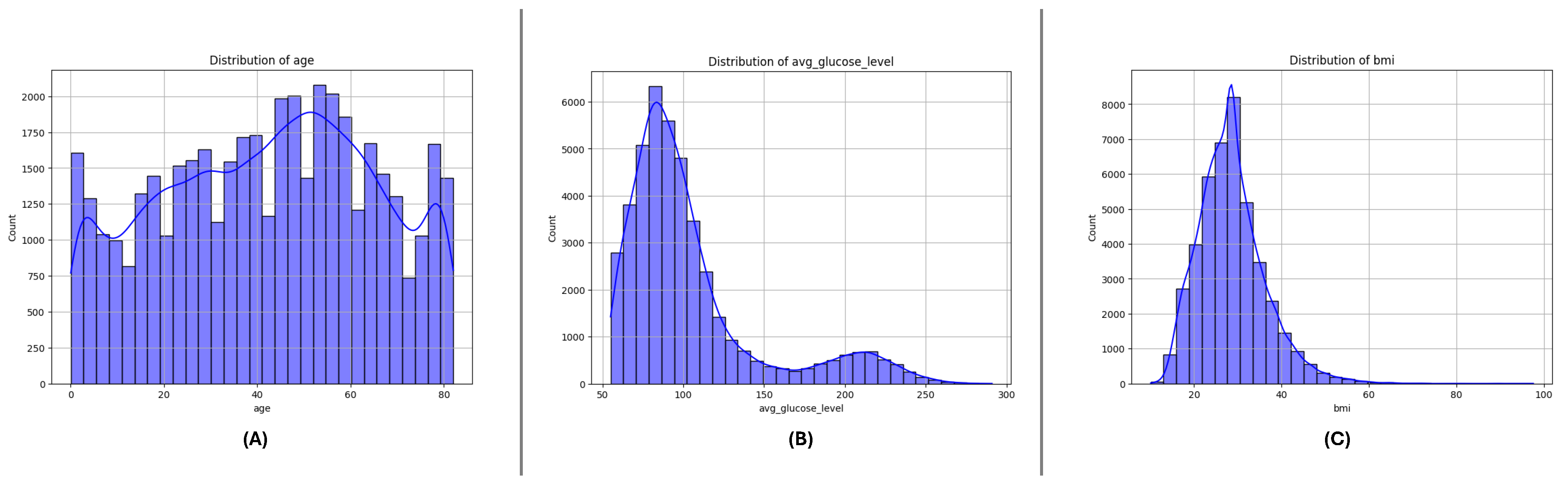
Figure 5.
DiDistributionf key numerical features in the DF-2 dataset: (A) Age, (B) Average glucose level, and (C) Body Mass Index (BMI). Patterns reveal significant variations across stroke and non-stroke populations.
Figure 5.
DiDistributionf key numerical features in the DF-2 dataset: (A) Age, (B) Average glucose level, and (C) Body Mass Index (BMI). Patterns reveal significant variations across stroke and non-stroke populations.
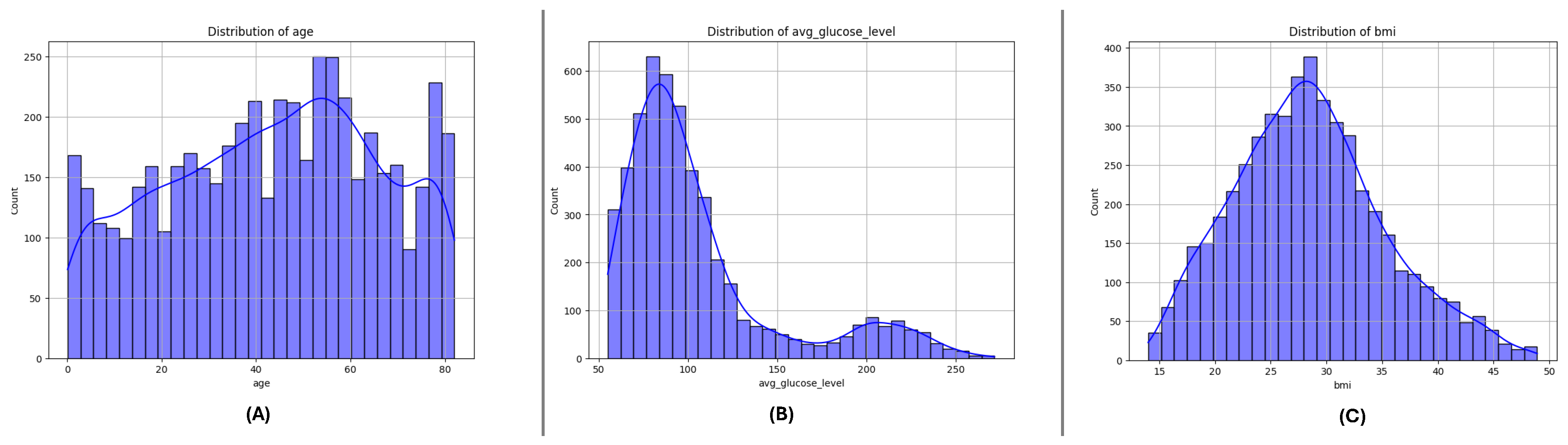
Figure 6.
DiDistributionf key numerical features in the DF-3 dataset: (A) Age, (B) Average glucose level, and (C) Body Mass Index (BMI). Notable trends and outliers provide insights into the dataset characteristics.
Figure 6.
DiDistributionf key numerical features in the DF-3 dataset: (A) Age, (B) Average glucose level, and (C) Body Mass Index (BMI). Notable trends and outliers provide insights into the dataset characteristics.
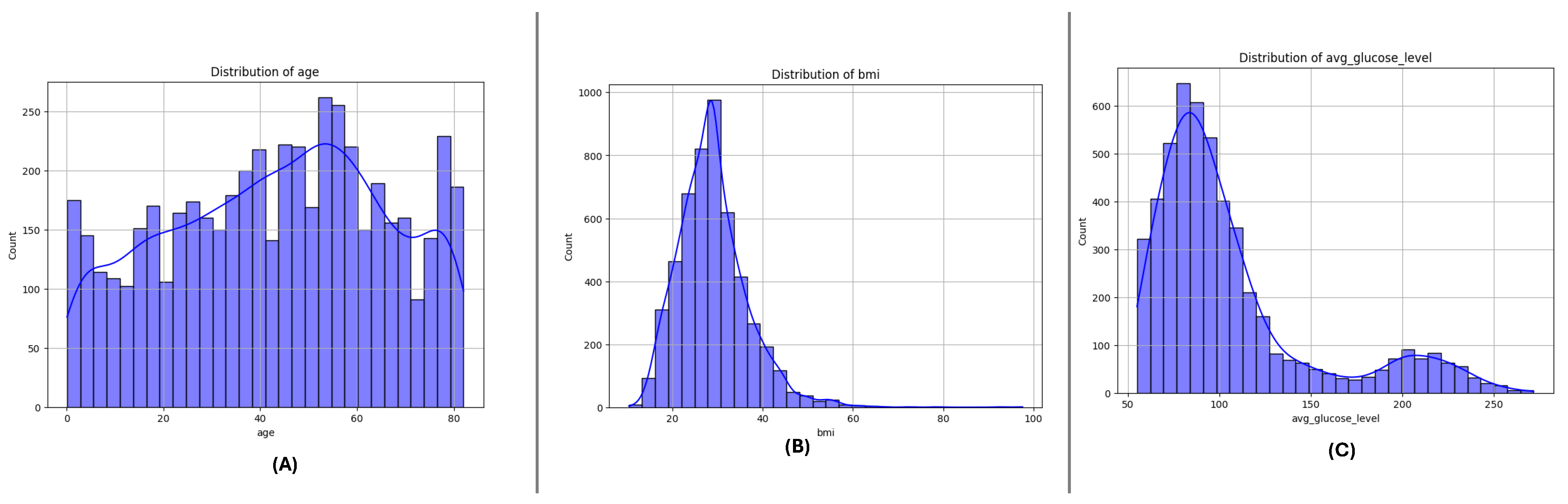
Figure 7.
Correlation matrix of the DF-1 dataset showing relationships between features after one-hot encoding. High correlations (absolute values near 1) indicate redundancy and features exceeding the threshold of 0.8 were removed.
Figure 7.
Correlation matrix of the DF-1 dataset showing relationships between features after one-hot encoding. High correlations (absolute values near 1) indicate redundancy and features exceeding the threshold of 0.8 were removed.
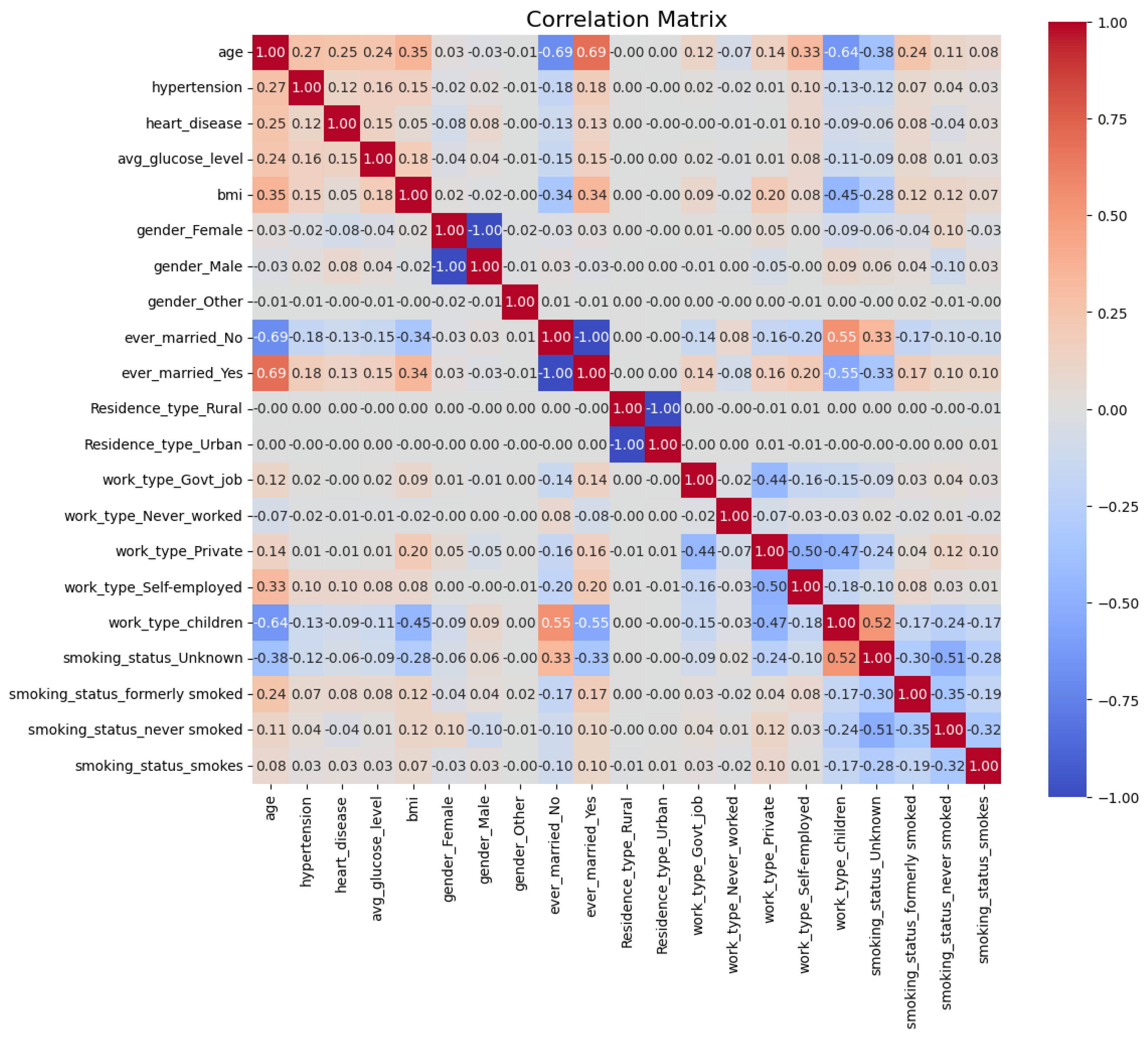
Figure 8.
F1 Score vs. Number of Selected Features (k). The optimal is indicated by the vertical dashed line.
Figure 8.
F1 Score vs. Number of Selected Features (k). The optimal is indicated by the vertical dashed line.
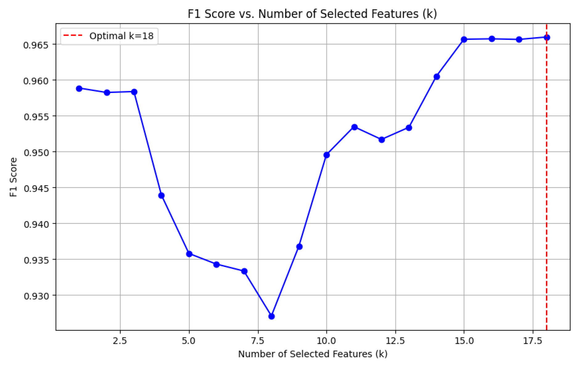
Figure 9.
Proposed meta-learning framework: base models generate initial predictions, and the meta-model combines and refines these outputs to produce the final prediction.
Figure 9.
Proposed meta-learning framework: base models generate initial predictions, and the meta-model combines and refines these outputs to produce the final prediction.
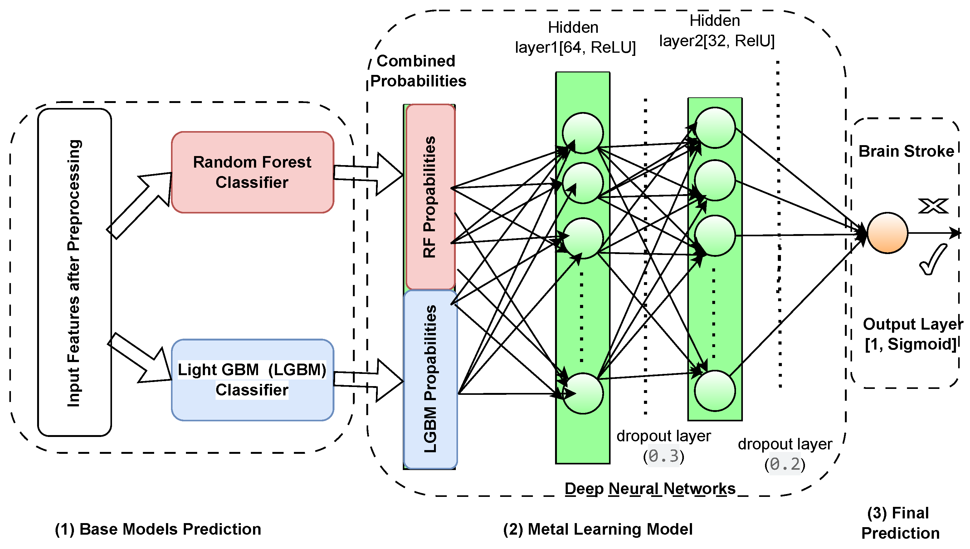
Figure 10.
Precision-Recall curve for DF-1 dataset using imbalance handling methods: (A) SMOTE, (B) SMOTEEN, and (C) SMOTE-SMOTEEN.
Figure 10.
Precision-Recall curve for DF-1 dataset using imbalance handling methods: (A) SMOTE, (B) SMOTEEN, and (C) SMOTE-SMOTEEN.
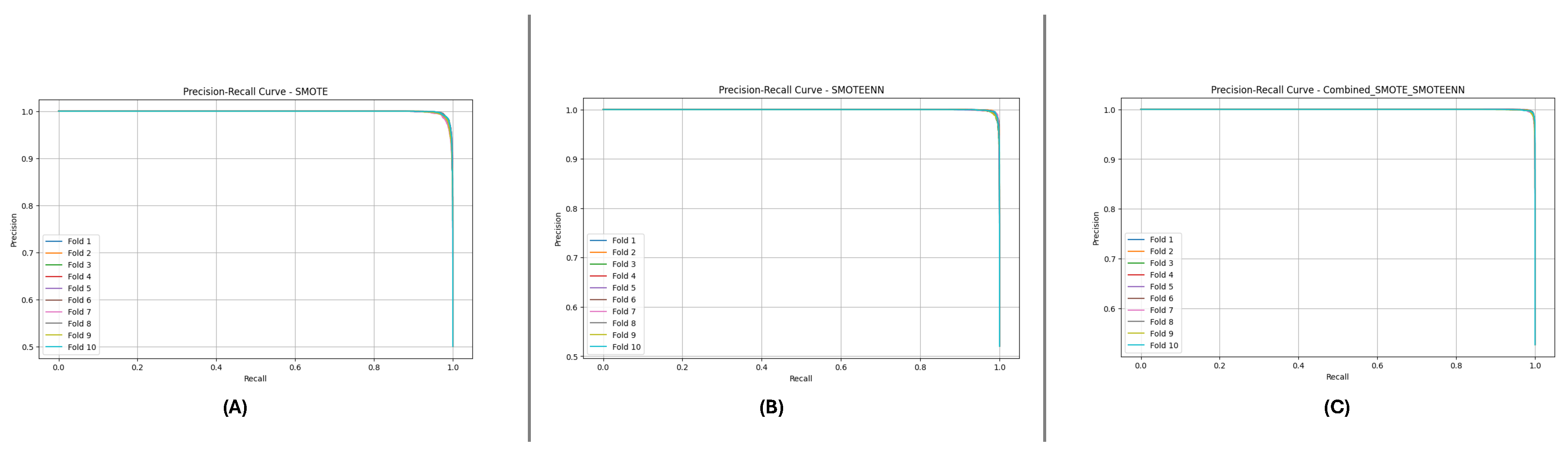
Figure 11.
ROC-AUC curve for DF-1 dataset using imbalance handling methods: (A) SMOTE, (B) SMOTEEN, and (C) SMOTE-SMOTEEN.
Figure 11.
ROC-AUC curve for DF-1 dataset using imbalance handling methods: (A) SMOTE, (B) SMOTEEN, and (C) SMOTE-SMOTEEN.
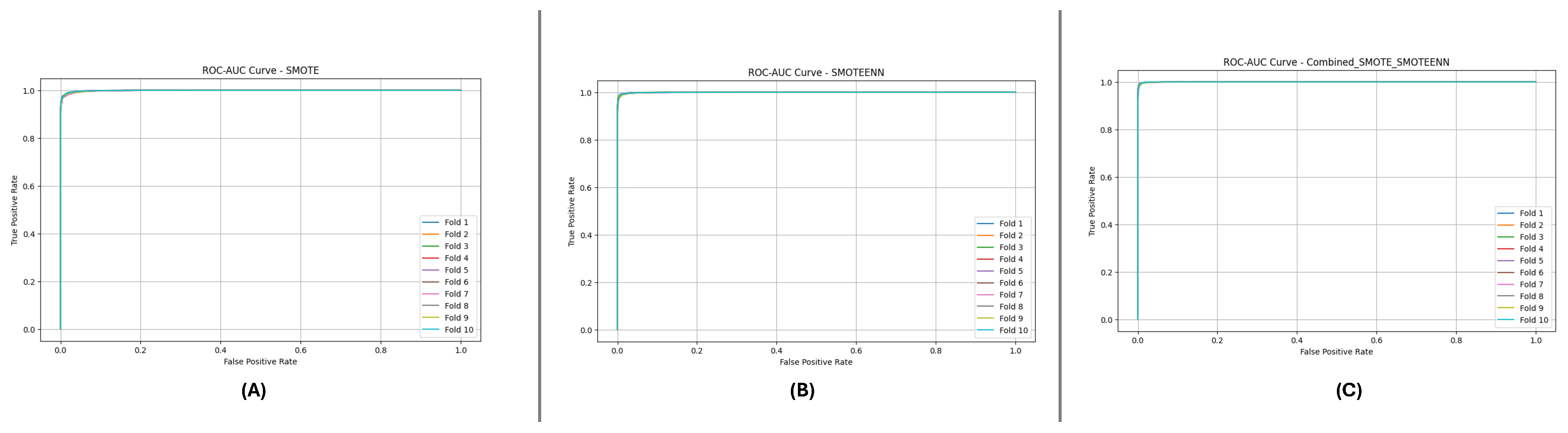
Figure 12.
Precision-Recall curve for DF-2 dataset using imbalance handling methods: (A) SMOTE, (B) SMOTEEN, and (C) SMOTE-SMOTEEN.
Figure 12.
Precision-Recall curve for DF-2 dataset using imbalance handling methods: (A) SMOTE, (B) SMOTEEN, and (C) SMOTE-SMOTEEN.
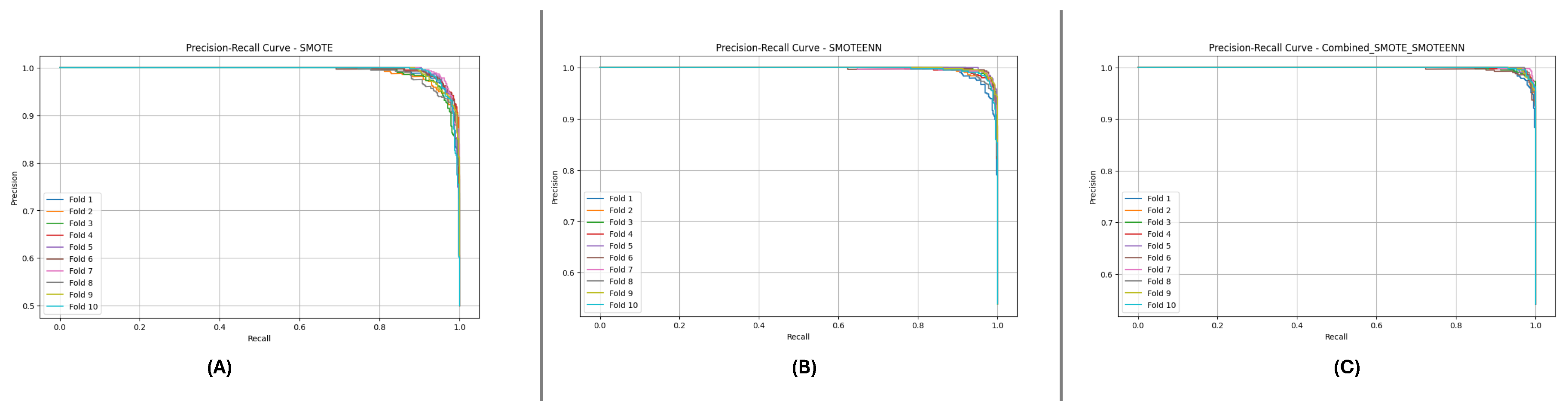
Figure 13.
ROC-AUC curve for DF-2 dataset using imbalance handling methods: (A) SMOTE, (B) SMOTEEN, and (C) SMOTE-SMOTEEN.
Figure 13.
ROC-AUC curve for DF-2 dataset using imbalance handling methods: (A) SMOTE, (B) SMOTEEN, and (C) SMOTE-SMOTEEN.
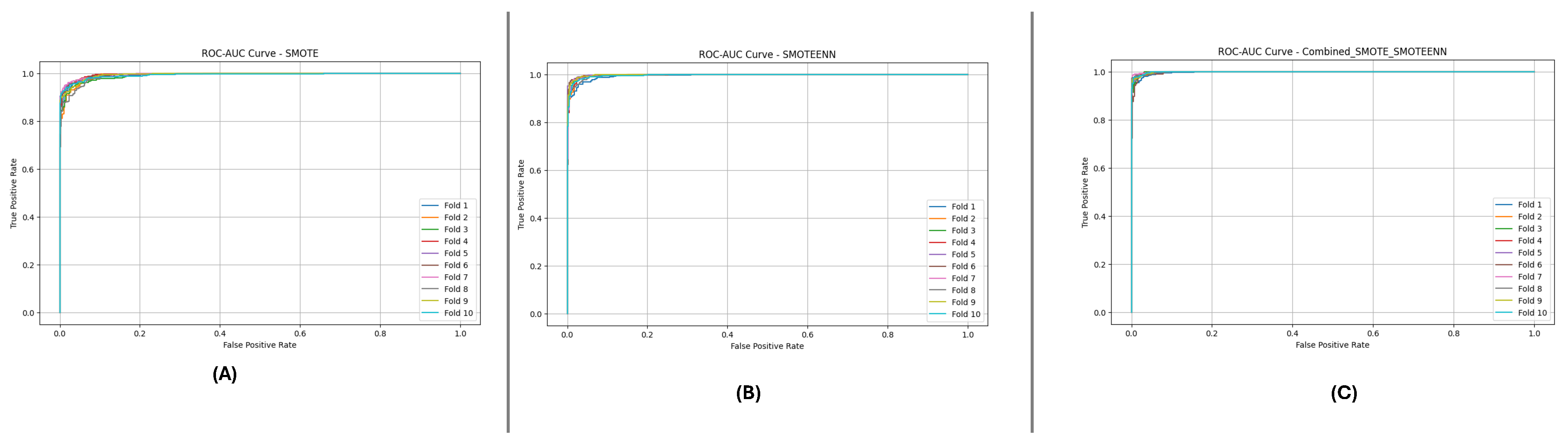
Figure 14.
Precision-Recall curve for DF-3 dataset using imbalance handling methods: (A) SMOTE, (B) SMOTEEN, and (C) SMOTE-SMOTEEN.
Figure 14.
Precision-Recall curve for DF-3 dataset using imbalance handling methods: (A) SMOTE, (B) SMOTEEN, and (C) SMOTE-SMOTEEN.
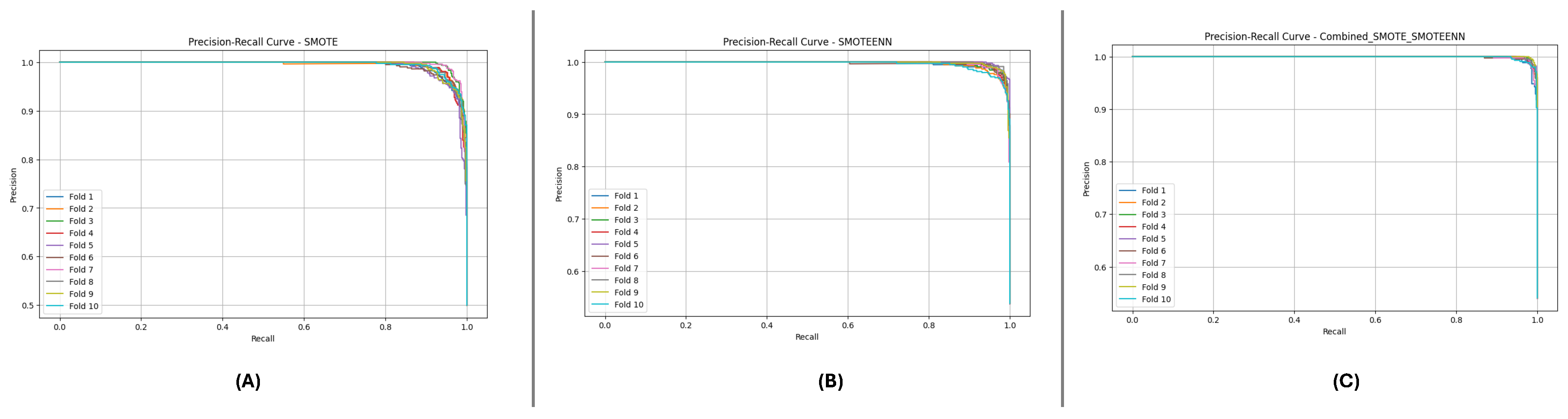
Figure 15.
ROC-AUC curve for DF-3 dataset using imbalance handling methods: (A) SMOTE, (B) SMOTEEN, and (C) SMOTE-SMOTEEN.
Figure 15.
ROC-AUC curve for DF-3 dataset using imbalance handling methods: (A) SMOTE, (B) SMOTEEN, and (C) SMOTE-SMOTEEN.
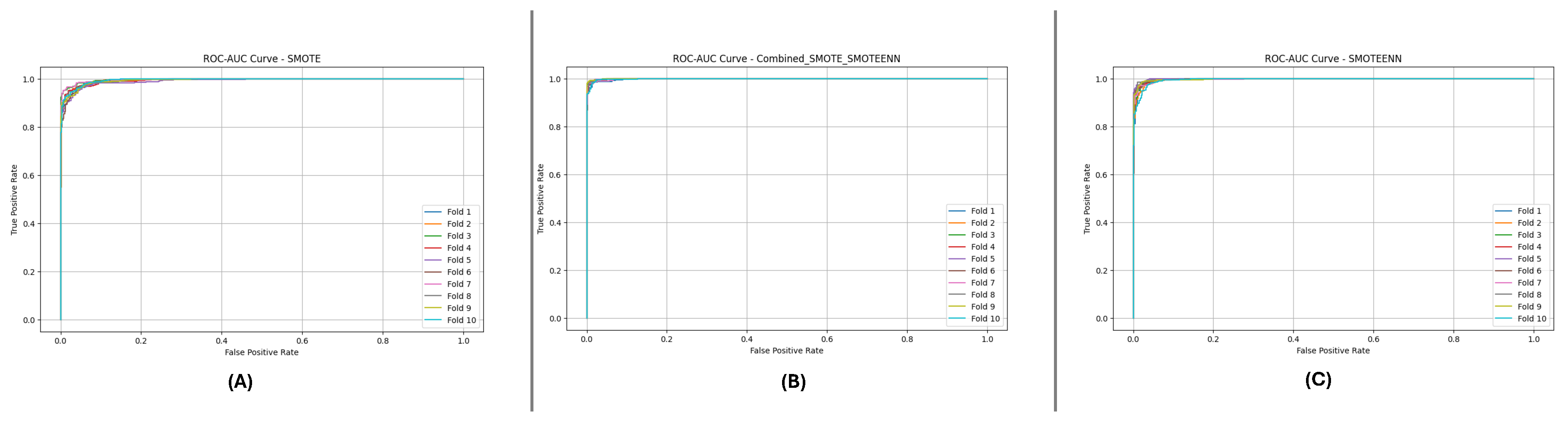
Figure 16.
Global feature importance using SHAP for the datasets: (A) DF-1, (B) DF-2, and (C) DF-3.
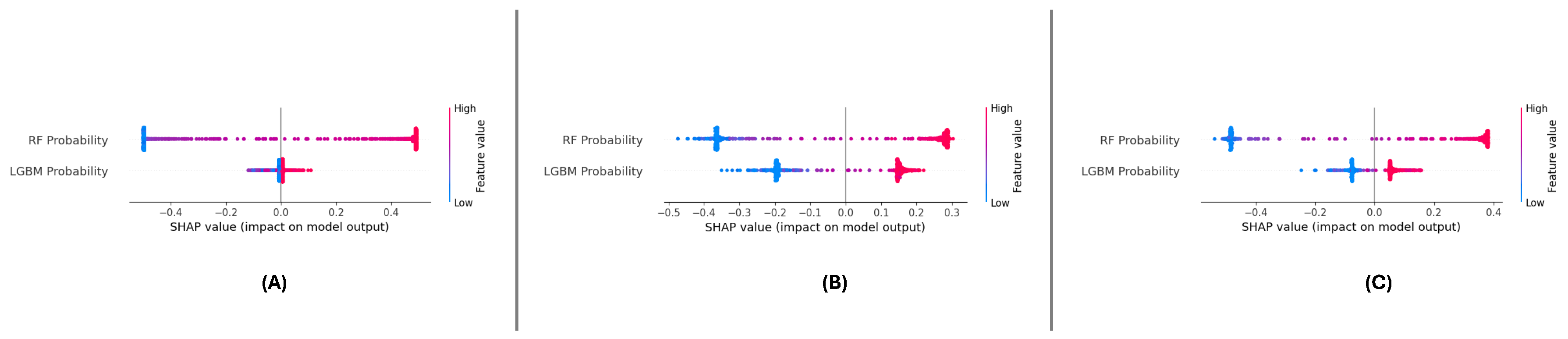
Figure 17.
Feature dependency and interaction or the datasets: (A) DF-1, (B) DF-2, and (C) DF-3 datasets.
Figure 17.
Feature dependency and interaction or the datasets: (A) DF-1, (B) DF-2, and (C) DF-3 datasets.
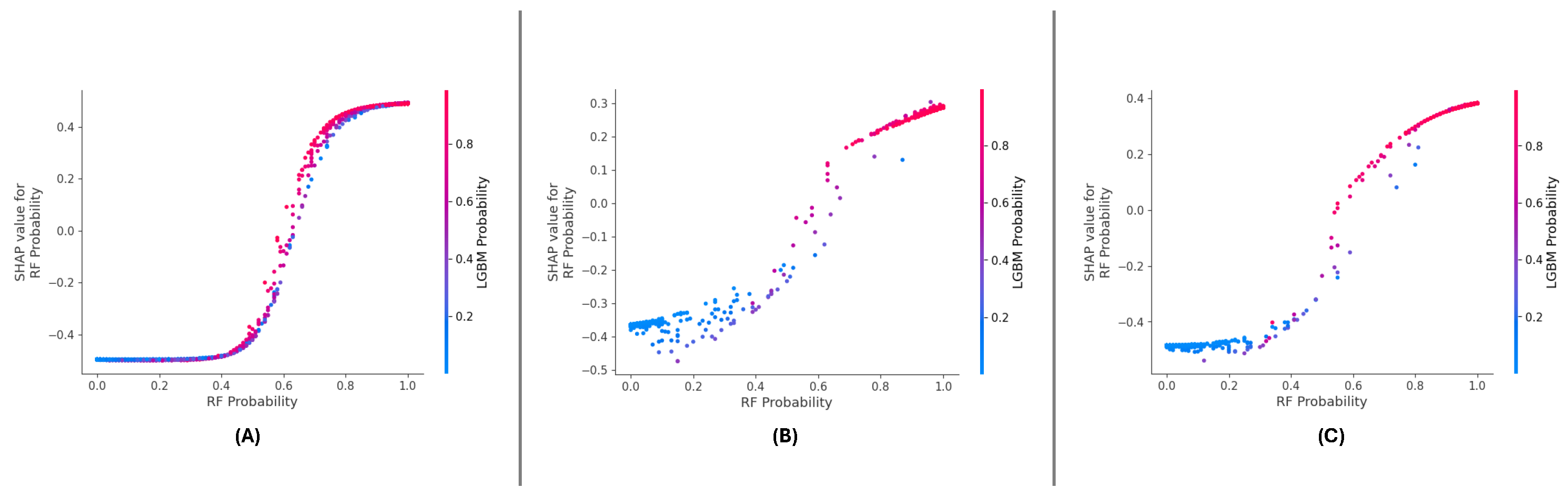
Figure 18.
Localized explanations using SHAP force plots for individual predictions in the datasets: (A) DF-1, (B) DF-2, and (C) DF-3.
Figure 18.
Localized explanations using SHAP force plots for individual predictions in the datasets: (A) DF-1, (B) DF-2, and (C) DF-3.

Figure 19.
Cumulative feature contributions visualized through SHAP decision plots for the datasets: (A) DF-1, (B) DF-2, and (C) DF-3.
Figure 19.
Cumulative feature contributions visualized through SHAP decision plots for the datasets: (A) DF-1, (B) DF-2, and (C) DF-3.
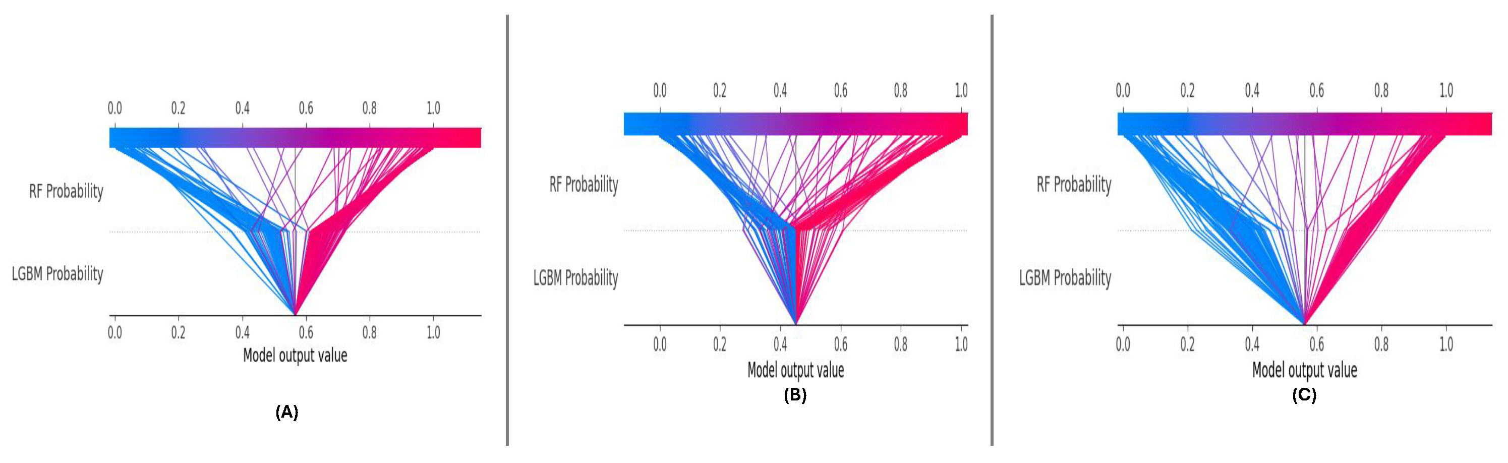
Table 1.
Description of Dataset Fields in DF1 and DF2.
| Feature Name | Description | Type |
|---|---|---|
| age | Patient’s age in years | Numeric |
| Gender | Gender of the patient (Male, Female) | Categorical |
| hypertension | Whether the patient has hypertension (0 or 1) | Binary |
| heart_disease | Presence of heart disease (0 or 1) | Binary |
| ever_married | Marital status (Yes, No) | Categorical |
| work_type | Type of work (Private, Self-employed, etc.) | Categorical |
| Residence_type | Area of residence (Urban, Rural) | Categorical |
| avg_glucose_level | Average glucose level in blood | Numeric |
| bmi | Body Mass Index (BMI) | Numeric |
| smoking_status | Smoking status (Never smoked, Smokes, etc.) | Categorical |
| stroke | Stroke occurrence (Target: 0 or 1) | Binary |
Table 2.
Class Distribution in DF-1, DF-2, and DF-3.
| Dataset | Class | Samples | Percentage (%) |
|---|---|---|---|
| DF-1 [29] | Non-Stroke (0) | 42,617 | 98.2% |
| Stroke (1) | 783 | 1.8% | |
| DF-2 [30] | Non-Stroke (0) | 4,733 | 95.0% |
| Stroke (1) | 248 | 5.0% | |
| DF-3 [31] | Non-Stroke (0) | 4,861 | 95.1% |
| Stroke (1) | 249 | 4.9% |
Table 3.
Features Introduced by One-Hot Encoding
| Feature | Description |
|---|---|
| gender_Female | Indicates if the gender is Female (binary: 0 or 1). |
| gender_Male | Indicates if the gender is Male (binary: 0 or 1). |
| gender_Other | Indicates if the gender is Other (binary: 0 or 1). |
| ever_married_No | Indicates if the individual has never married (binary: 0 or 1). |
| ever_married_Yes | Indicates if the individual has been married (binary: 0 or 1). |
| Residence_type_Rural | Indicates if the residence type is Rural (binary: 0 or 1). |
| Residence_type_Urban | Indicates if the residence type is Urban (binary: 0 or 1). |
| work_type_Govt_job | Indicates if the work type is Government job (binary: 0 or 1). |
| work_type_Never_worked | Indicates if the individual has never worked (binary: 0 or 1). |
| work_type_Private | Indicates if the work type is Private sector (binary: 0 or 1). |
| work_type_Self-employed | Indicates if the work type is Self-employed (binary: 0 or 1). |
| work_type_children | Indicates if the work type is related to children (binary: 0 or 1). |
| smoking_status_Unknown | Indicates if the smoking status is unknown (binary: 0 or 1). |
| smoking_status_formerly smoked | Indicates if the individual formerly smoked (binary: 0 or 1). |
| smoking_status_never smoked | Indicates if the individual never smoked (binary: 0 or 1). |
| smoking_status_smokes | Indicates if the individual currently smokes (binary: 0 or 1). |
Table 4.
Summary of evaluation metrics and their equations.
| Metric | Description | Equation |
|---|---|---|
| Accuracy | Proportion of correct predictions among all cases. | |
| Precision | Proportion of true positives among all positive predictions. | |
| Recall (Sensitivity) | Proportion of true positives among all actual positives. | |
| F1 Score | Harmonic mean of Precision and Recall. | |
| ROC-AUC | Area under the ROC curve. | |
| Cohen Kappa | Agreement between predicted and actual labels, adjusted for chance. |
Table 5.
Performance comparison on DF-1 dataset
| SMOTE | SMOTEENN | SMOTE_SMOTEENN | ||||
|---|---|---|---|---|---|---|
| Mean | Std. | Mean | Std. | Mean | Std. | |
| Accuracy | 0.983739 | 0.001473 | 0.989341 | 0.000959 | 0.992189 | 0.001142 |
| Precision | 0.984304 | 0.003651 | 0.989271 | 0.002561 | 0.993501 | 0.001254 |
| Recall | 0.983176 | 0.003628 | 0.990264 | 0.002680 | 0.991661 | 0.002118 |
| F1-Score | 0.983730 | 0.001471 | 0.989762 | 0.000921 | 0.992579 | 0.001090 |
| ROC AUC | 0.998856 | 0.000226 | 0.999460 | 0.000097 | 0.999728 | 0.000076 |
| Cohen Kappa | 0.967478 | 0.002945 | 0.978645 | 0.001921 | 0.984334 | 0.002290 |
Table 6.
Performance comparison on DF-2 dataset
| SMOTE | SMOTEENN | SMOTE_SMOTEENN | ||||
|---|---|---|---|---|---|---|
| Mean | Std. | Mean | Std. | Mean | Std. | |
| Accuracy | 0.956792 | 0.005906 | 0.974961 | 0.0076 | 0.980297 | 0.00248 |
| Precision | 0.953499 | 0.008228 | 0.972186 | 0.011668 | 0.976108 | 0.001943 |
| Recall | 0.960494 | 0.007696 | 0.981709 | 0.00409 | 0.987795 | 0.003084 |
| F1-Score | 0.956956 | 0.005844 | 0.976893 | 0.006891 | 0.981916 | 0.002295 |
| ROC AUC | 0.993853 | 0.001366 | 0.997314 | 0.001116 | 0.998717 | 0.000552 |
| Cohen Kappa | 0.913585 | 0.011811 | 0.94957 | 0.015352 | 0.960277 | 0.004993 |
Table 7.
Performance comparison on DF-3 dataset
| SMOTE | SMOTEENN | SMOTE_SMOTEENN | ||||
|---|---|---|---|---|---|---|
| Mean | Std. | Mean | Std. | Mean | Std. | |
| Accuracy | 0.957828 | 0.005484 | 0.974077 | 0.006032 | 0.9934901 | 0.005255 |
| Precision | 0.955037 | 0.006166 | 0.970695 | 0.008552 | 0.97696 | 0.007958 |
| Recall | 0.960912 | 0.006294 | 0.981486 | 0.006761 | 0.989877 | 0.002184 |
| F1-Score | 0.957957 | 0.005471 | 0.976034 | 0.005543 | 0.983365 | 0.004762 |
| ROC AUC | 0.994063 | 0.001678 | 0.997051 | 0.00106 | 0.998943 | 0.000543 |
| Cohen Kappa | 0.915656 | 0.010968 | 0.947807 | 0.012157 | 0.963522 | 0.010617 |
Disclaimer/Publisher’s Note: The statements, opinions and data contained in all publications are solely those of the individual author(s) and contributor(s) and not of MDPI and/or the editor(s). MDPI and/or the editor(s) disclaim responsibility for any injury to people or property resulting from any ideas, methods, instructions or products referred to in the content. |
© 2025 by the authors. Licensee MDPI, Basel, Switzerland. This article is an open access article distributed under the terms and conditions of the Creative Commons Attribution (CC BY) license (http://creativecommons.org/licenses/by/4.0/).
Copyright: This open access article is published under a Creative Commons CC BY 4.0 license, which permit the free download, distribution, and reuse, provided that the author and preprint are cited in any reuse.


