Submitted:
23 October 2024
Posted:
24 October 2024
You are already at the latest version
Abstract
Dementia is a group of detrimental diseases and conditions that damage the human brain and impair mental functioning. In recent years, significant efforts have been made to develop robust computer-aided diagnostic tools, particularly AI models for detection. However, their clinical implementation remains limited. One issue identified is that despite achieving high accuracy, AI-powered predictions have relied on single features or small sets of features in limited categories, hindering their robustness and generalizability. Moreover, the accuracy alone has not been sufficient to convince medical practitioners to adopt these tools, as they require transparent and scientifically grounded diagnostic processes. This study aims to improve the transparency and reliability of AI models in predicting dementia through three key steps: 1) compare a Machine Learning (ML) model's accuracy in detecting dementia when trained on a multi-domain dataset to when trained on subsets of features, 2) evaluate additional ML models for dementia detection using the multi-domain dataset, and 3) apply Explainable AI (XAI) to elucidate the importance of specific features in ML-based predictions, thereby enhancing transparency and interpretability. We hypothesize that utilizing multi-domain data will enhance the performance of ML models. Furthermore, XAI will demonstrate that features with high influence on the model's decisions are aligned with established indicators of dementia. This study contributes to the field by constructing lightweight predictive models that deliver highly accurate performance while enhancing transparency and interpretability, advancing toward clinically applicable AI-powered diagnosis.
Keywords:
explainable AI (XAI)
; dementia
; class imbalance
; SHAP (SHapley Additive exPlanations)
; machine learning
; AI transparency
1. Introduction
Dementia is a term to describe diseases and medical conditions that affect the human brain and cause increasingly serious effects on patients’ physical, cognitive, and emotional health as they progress Arango Lasprilla et al. (2009). According to the World Health Organization, 55 million people are currently living with dementia, 60% of which come from low-and-middle-income nations dem (2023). Economically, in 2019, the global annual societal costs of dementia were estimated at $1313.4 billion, including direct medical expenses (16%), direct social sector costs (34%), and informal care (50%) Wimo et al. (2023). Several dementia-related diseases, namely Alzheimer’s Disease, Parkinson’s Disease, and Huntington’s Disease, are incurable and irreversible.
In recent years, the rise of research in Artificial Intelligence (AI) has introduced novel tools capable of automating the dementia diagnosis process with remarkable accuracy. These technologies can be classified based on the AI techniques used, such as Machine Learning (Logistic Regression, Decision Tree, Support Vector Machine (SVM), k-nearest-neighbor (kNN)) or Deep Learning (Convolutional Neural Network (CNN), Transformers), or based on the data used for prediction, including clinical indices, brain scans, or natural language. Each of these approaches has achieved varying levels of success in building robust models for early dementia prediction. For instance, Zhu et al. (2020) conducted a comparative analysis of six machine-learning algorithms for detecting dementia based on survey responses, resulting in an optimal model that scored over 0.8 in all evaluation metrics. Similarly, Amini et al. (2023) applied Natural Language Processing (NLP) to classify subjects in the Framingham Heart Study as normal, demented, or having mild cognitive impairment based on their automatically transcribed digital voice recordings from neuropsychological tests. This study demonstrated high accuracy in distinguishing between Normal, MCI, and Dementia subjects, showcasing the potential of NLP in dementia detection.
Despite successes in scientific settings and the increasing variety of techniques, AI models are rarely implemented in real-world clinical predictions. The main reason is that most studies focus on increasing the models’ accuracy while neglecting their applicability. Many models rely on small-sized datasets that lack feature diversity. For instance, machine learning approaches usually employ subjects’ results in cognitive tests, like the Mini-Mental State Exam (MMSE), to detect dementia. While this is not inaccurate, socioeconomic, demographic, and biological aspects also affect the risk of dementia McCullagh et al. (2001). Likewise, deep-learning-based models are trained to make predictions on brain scans, which have been claimed to be insufficient for training models to make reliable predictions for neurodegenerative diseases Oxtoby et al. (2017). Additionally, these models are often called `black-box models’ as their complex decision-making processes lack transparency and interpretability and are not entrusted by practitioners in not just healthcare, but also other fields, such as e-commerce, banking, public services, and safety Hassija et al. (2024).
Given these obstacles, a new field of study emerged - eXplainable AI (XAI). XAI is a set of techniques that are applied to AI models to illustrate their reasoning, outcomes, and potential bias in making decisions. In the context of healthcare technologies and disease detection specifically, XAI is usually employed to illustrate the factors that influence a model’s classification of each subject into a category (e.g.: demented or non-demented). If XAI shows that a factor’s influence on the model’s classification is similar to its proven influence on disease risk, the model can be considered potentially reliable and transparent to practitioners’ usage. XAI is a new field of interest in recent years and has yet to be fully utilized. In healthcare, Loh et al. (2022) asserted that there have only been 141 XAI studies published in quartile-ranked journals, 99 of which are in Q1 journals.
Employing machine-learning-based predictions and XAI, this study aims to tackle the two main problems underlying the lack of implementation of AI-powered predictions in real-world clinical settings: the reliance of models on a narrow set of features and the lack of transparency in their predictions. To tackle these problems, we train an initial baseline model to investigate the influence of domain variety on AI-powered dementia detection. Additional ML models were subsequently trained and compared to identify the best-performing model on this task, and finally, we applied SHapley Additive exPlainations (SHAP) - an XAI technique to illustrate the influence of each feature on the decision-making process of the best-performing classifier for each label. We hypothesized that 1) the domain variety of a dataset helps enhance the performance of ML classifiers and 2) SHAP would indicate that factors that have been proven to have a positive or negative effect on dementia risk, in reality, would have the same effect in the decision-making process of the classifier. By following this multi-step procedure, this study aims to tackle the main problems of current predictive models, reliance on limited or narrow data and lack of transparency, thereby endorsing their clinical adoptions.
2. Literature Review
Research in dementia diagnosis has been continuously rising, with the constant emergence of new technologies. From traditional machine learning (ML) approaches, researchers have expanded into using state-of-the-art deep learning techniques, such as computer vision (e.g., disease detection via brain scans) and natural language processing (e.g., language anomaly detection). Each of these approaches has achieved significant success in testing, showcasing the potential for standardizing and automating the dementia detection process. Zhu et al. (2020) compared six machine-learning techniques for detecting dementia on imbalanced clinical data. The researchers applied three feature selection methods—Random Forest, Information Gain, and Relief—to reconstruct the dataset and trained the models on six algorithms, including Random Forest, AdaBoost, LogitBoost, Neural Network (NN), Naive Bayes, and Support Vector Machine (SVM). Their findings concluded that Naive Bayes performed best, achieving 0.81 accuracy, 0.82 precision, 0.81 recall, and 0.81 F-measure. However, this study focused on performance based on either all 37 features or a reduced set of two selected features. While beneficial for performance, this reduction led to a loss of data diversity, limiting the potential insights into how different data domains influence ML-based decision-making
In Deep Learning, Choi et al. (2018) explored the use of Convolutional Neural Networks (CNNs) to predict the progression of Mild Cognitive Impairment (MCI) to Alzheimer’s Disease (AD), the most common dementia-related condition (Kawas & Corrada, 2006). The study used PET images of 139 AD patients, 171 MCI patients, and 182 normal subjects from the Alzheimer’s Disease Neuroimaging Initiative database. A deep CNN was trained on these 3D images to predict MCI progression to AD, with the model achieving 84.2% accuracy on the test set, significantly outperforming traditional feature-based approaches. However, Oxtoby et al. (2017) critiqued the reliance on neuroimaging alone, suggesting that it is insufficient as an independent ground for making reliable predictions in the context of neurodegenerative diseases, including dementia. This critique emphasizes the limitations of models trained on a single data source, underscoring the need for models that consider a broader range of features.
Despite these advancements, many AI models have struggled with real-world clinical implementation. This is partly due to a narrow focus on accuracy at the expense of reliability and applicability. Models often fail to account for the diversity of features influencing dementia, such as demographic, socioeconomic, and cognitive factors. The limited range of features used in training AI models makes their predictions less reliable because dementia is an acquired condition influenced by various factors. First, demographic and socioeconomic factors have been shown to significantly impact dementia risk. Firstly, demographic and socioeconomic factors have also been proven to be influential on the dementia risk. In their study, Prince et al. (2015) emphasized the strong correlation between demographic factors and dementia: People with a higher level of education are associated with a lower risk of dementia.
Meanwhile, neurobiological factors, including brain volume and biomarkers, have also been proven critical in understanding dementia. Reduced brain volume, particularly in regions such as the hippocampus, has been consistently linked to the progression of Alzheimer’s disease and other forms of dementia. Studies have shown that hippocampal atrophy is one of the earliest and most reliable indicators of Alzheimer’s disease, with significant volume reduction observable in patients even before clinical symptoms manifest Jack Jr et al. (1999).
Lastly, cognitive performance, assessed through various neuropsychological tests, is a direct indicator of dementia. Tests such as the Mini-Mental State Examination (MMSE) are commonly used to evaluate cognitive decline. Folstein et al. (1975) introduced the MMSE, a widely used cognitive test containing 30 questions in clinical settings for measuring cognitive loss. This assessment measures various cognitive domains and is strongly predictive of dementia’s onset and progression Jack Jr et al. (2011).
Given this background, it is clear that training AI models for dementia diagnosis on a limited set of features is inadequate. By considering a broad set of features, predictive models can more effectively capture the complexity of dementia, thereby increasing the comprehensiveness of AI-powered diagnosis. As this understanding has grown, researchers have begun to incorporate a wider range of features into their datasets to enhance model performance and interpretability.
Aditya and Pande (2017) employed a novel approach by training a supervised model to detect Alzheimer’s Disease (AD) based on interactions among various features in a high-dimensional dataset without neuroimaging. Using an adapted version of the Open Access Series of Imaging Studies (OASIS), they trained a supervised Multifactor Affiliation Analysis model to effectively capture complex feature interactions in the sample space of AD data. This model quantified the similarity of test subjects to the demented class by assessing the affiliation across various features and calculating multifactor-affiliation weights based on feature interactions. Although this study enhanced model interpretability by verifying the model’s conception of feature interrelation, it focused primarily on exploring the correlation between features rather than providing insights into the importance of individual features in ML-based decision-making.
To address the issue of limited interpretability, studies in AI-powered diagnosis increasingly adopt Explainable AI (XAI) techniques. XAI helps to clarify the decision-making process of ML models, thereby enhancing their transparency and applicability in clinical practice.
Recently, Xue et al. (2024) employed XAI to elucidate the decision-making process of their transformer-based model for detecting various types of dementia. Although the study achieved high performance, with AUROC scores of 0.96 for weighted-average, 0.91 for macro-average, and 0.94 for weighted average, the dataset’s features were predominantly biological, with a minority representing demographic data. This imbalance limited the diversity of the study’s dataset, potentially reducing the effectiveness of SHAP in equally demonstrating the importance of each feature. Additionally, one of the biggest drawbacks of Deep Learning models is the enormous amount of data they require for training Bansal et al. (2022). In this study, the researchers had to combine 9 different datasets into a joint dataset with over 50000 subjects to enhance the robustness and accuracy of their deep neural network.
In summary, while AI and machine learning models have shown promise in dementia detection, their clinical applicability remains limited due to narrow feature sets, lack of transparency, and the need for extensive data. Future research should focus on integrating diverse, multi-domain datasets and employing XAI techniques to enhance both the performance and interpretability of models, paving the way for their adoption in clinical settings.
3. Methodology
3.1. Introduction
In this paper, we examine the significance of domain variety, the performance across Machine Learning models in dementia detection, and the feature importance of demographic, socioeconomic, neurobiological, and cognitive measures in the detection. The dataset used for all phases of the experiment was the adapted version of the Open Access Series of Imaging Studies (OASIS-2) which excluded neuroimaging components for Machine Learning use. To deal with the class imbalance and domain variety in the dataset, 4 models were selected for training, validation, and comparison: Random Forest Classifier, Support Vector Machine, k-Nearest-Neighbor, and XGBoost. After comparison, the model with the best performance underwent the implementation of SHapley Additive exPlanations (SHAP), an XAI technique, that illustrated the contribution of all features to the classification of each Clinical Dementia Rating (CDR) label.
3.2. Dataset
3.2.1. Origin
The Open Access Series of Imaging Studies (OASIS-2) is the second version of the OASIS database (Marcus et al, 2010). This database consists of 150 subjects aged from 60 to 96 and is a part of larger MRI studies conducted at the Washington University Knight Alzheimer Disease Research Center (Knight ADRC). In the OASIS-2 dataset, for each subject, 3 or 4 individual T1-weighted MRI brain scans were collected. The dataset included both male and female participants, all of which were right-handed. At the end of the study, 150 participants resulted in 373 total instances (data points). Comparing the diagnosis of the subjects before and after the study, the researchers concluded that there were 72 demented, 64 non-demented, and 14 subjects whose diagnosis was converted (from non-demented to demented).
In this study, an adapted version of the OASIS-2 dataset, which excludes the neuroimaging data of the participants, was employed. Battineni et al. (2019) first proposed this dataset as a lightweight adapted resource to facilitate studies in ML-based dementia prediction on multi-domain data. Apart from excluding neuroimaging data, this adaptation retained all features of the original dataset. For this study only, the Identification (ID) of each patient was excluded and each visit was treated as an independent data point to increase the size of the dataset from 150 to 373 instances, giving more capacity for model training and validation.
3.2.2. Feature Selection and Domain Categorization
The dataset consists of 15 columns in total. The target column is the Clinical Dementia Rating (CDR), thus this column was not included in the feature selection. In the remaining, we decided to choose 7 features, classified into 3 domains: demographic and socioeconomic, neurobiological, and cognitive data. The name of each feature, their abbreviation in the original study, and the domain they belong to are shown in Table 1.
3.2.3. Data Analysis
Among the 373 instances in the original dataset, there are 19 rows where the socioeconomic status (SES) is a null value, 2 of which also have null values for the MMSE score. Since this amount of data is not considerable compared to the size of the dataset, we decided to exclude all these 19 data points. Consequently, the final dataset contains 354 data points in total.
Subsequently, apart from the presence of null values, the target (CDR) suffers from great class imbalance. CDR instances in the dataset fall into one of the following values: 0, 0.5, 1, or 2. Before analysis, class 0 dominated the dataset, encompassing 206 data points in total. Meanwhile, class 2 had the fewest share, only 3 over 354 data points. In training the machine learning models, such great data imbalance can lead to model bias and pretentious performance (Guo et al., 2008). In this study, we tackled this problem in three ways: reprocessed the classes, employed models with comparable capability of handling data imbalance, and utilized multiple evaluation metrics. Based on the meaning of class (0: cognitively normal, : slightly demented (slight risk of dementia), : high risk of dementia), we redistribute the dataset into 3 final classes: 0: cognitively normal, 1: slight risk, and 2: high risk. Figure 1 and Figure 2 show the distribution of CDR classes in the dataset before and after reprocessing.
After the analysis and reprocessing were completed, we split the dataset into 2 sets for training and validation, comprising 70% and 30% of the dataset, respectively.
3.2.4. Visualizations
As the last step in early data analysis, the value distribution of one feature in each domain was visualized for a better understanding. The visualizations of normalized whole brain volume, MMSE score, and education level are reflected in Figure 3, Figure 4, and Figure 5 respectively.
In addition, some keynote insights of the dataset in other features include:
- The age range of subjects is 38, with the youngest being 60 and the oldest being 98.
- The socioeconomic status (SES) index is recorded on a scale from 1 to 6, with 1 being the lowest and 6 being the highest. The most common socioeconomic status value is 2, which makes up nearly one-third of the dataset (103), while the number of people scoring 5 in SES is only 7.
- Estimated total intracranial volume values range from 1106 to 2004
3.3. Evaluation Metrics
3.3.1. Accuracy
Accuracy is a fundamental and simple evaluation metric that shows how accurately a model performs. It is calculated by the following formula:
In datasets with imbalanced class distributions, accuracy can be misleading because it does not account for the true distribution of class labels. Despite the preprocessing, the dataset in our study is still affected by the class imbalance, with non-demented instances being dominant. Accuracy, while a common metric, can be misleading in imbalanced datasets. Therefore, this study also employs precision, recall, and F1-score to provide a more comprehensive evaluation of model performance, particularly for minority classes.
3.3.2. Precision, Recall, F1-Score
In a dataset where some classes are larger than others, models tend to classify instances as those classes more. Precision tackles biased decision-making by calculating the proportion of instances classified as a class (positive) that belong to that class (true positive):
On the other hand, recall is a metric that evaluates how well a model captures the instances of each class:
In minor classes, the wrong classification of several instances may not significantly affect the overall accuracy but can heavily reduce the recall value of those classes. In this way, the recall metric helps the model avoid missing any instances due to biased assumptions during classification.
F1-Score is a harmonic mean of precision and recall, reflecting the model’s ability to correctly classify instances of a particular class while avoiding misclassification of instances from other classes into that class:
A good F1-Score means that the model can balance between precision and recall in generating classifications for a certain class.
To extract the final evaluations, macro(unweighted) averaging and weighted(weighted) averaging were applied to component scores in precision, recall, and F1-score of each class.
3.3.3. Averaging
Macro averaging works on the assumption that all classes in a dataset have equal importance in indicating the model’s performance:
Where: C is the number of classes
With this formula, the overall precision, recall, and F1-score are the mean of each class’s component precision, recall, and F1-score value respectively.
However, since even small errors can cause a high reduction in component scores of minor classes, macro averaging may need to be more accurate in the performance of the model. Weighted-averaging tackles this issue by assigning a weight to each class based on its statistical significance:
Where:
- is the weight (proportion) of the class i
- C is the number of classes
Using weighted-averaging ensures that the impact of a class’s component scores is relative to its data significance and that the final model evaluation is not strongly affected by minor classification errors.
3.4. Model Selection
To validate the significance of domain variety in a dataset in dementia prediction, an initial model is trained on the complete dataset, and then on sub-datasets with a single domain to highlight the margin in performance. Then, to further identify the best-performing model in imbalanced multilabel classification using the multi-domain dataset, 3 additional classifying models were trained. The performance of all 4 models was eventually compared based on the chosen evaluation metrics.
The 4 chosen models included 2 single models and 2 ensemble models. Ensemble models are models that either consist of multiple classifiers and conclude their predictions based on voting or learn from the knowledge of trained classifiers to make their predictions. The single models included are Support Vector Machine (SVM) and k-Nearest-Neighbor (kNN) and the ensemble models are Random Forest (RF) and XGBoost (XGB).
3.4.1. Random Forest Classifier
An RF classifier is an ensemble model constructed upon Decision Trees (DT) and performs prediction by letting all DTs predict on a different sample set of data and concluding the final output through majority voting. A decision tree starts with a node that contains instances from different classes. At each step, the current node will be split into 2 branch nodes in a way that optimizes the homogeneity of the majority classes. DT classifier executes this splitting by calculating the GINI Impurity:
Where: is the proportion of class i in the node
In each split, the DT tries to minimize the Gini Impurity by trying to group as many instances of the same class as possible into one node. After multiple splits, ideally, each of the final nodes, called leaves, will contain instances belonging to only one class. Class proportions are values that range from 0 to 1, whose squared values are smaller than the original values. This makes it harder for the Gini Impurity to reach 0 (highest purity) and the DT therefore must devise the best splitting strategy.
In an RF classifier, not all DTs will perform classification on the dataset, but each of them will classify a subset that was sampled with replacement, or bootstrapped. Specifically, each subset is sampled from the original dataset, but some instances are duplicated and as a result, some are excluded. This replacement is random and unique to the subset of each decision tree. The process helps create diversity among the DTs, ensuring that they do not make the same mistakes. The duplication of instances may cause overfitting among certain DTs, but the final classification of an instance is determined by majority voting among all DTs, so overfitting is avoided.
RF is an ensemble learning method known for its robustness and ability to handle large feature sets and complex data interactions. It was chosen as the baseline model due to its effectiveness in dealing with class imbalance through majority voting, which is particularly relevant for this study’s imbalanced dataset.
As the baseline model, an was trained on the multi-domain dataset and each domain separately to prove the significance of domain variety in dementia prediction. This RF classifier was constructed with 50 component DTs (. Subsequently, the RF’s performance was compared with 3 other classifiers to identify the best-performing model on multi-domain data.
3.4.2. Support Vector Machine
Support Vector Machine (SVM) is a powerful classifier, particularly powerful in high-dimensional spaces. SVM operates by finding the hyperplane that best separates instances of different classes in the feature space. The goal of the SVM is to maximize the margin, which is the distance between the hyperplane and the nearest data points from each class, known as support vectors. These support vectors are critical as they define the optimal separating hyperplane.
To handle cases where data points may overlap or where perfect separation is not possible, SVM introduces a regularization parameter C, controlling the trade-off between maximizing the margin and minimizing the classification error. A soft margin allows some misclassifications to occur, where the decision boundary is adjusted to find the optimal balance between margin width and error minimization. The objective function is to minimize:
Subject to the constraint:
and
Where:
- b is the bias term
- is the feature vector of the ith instance
- is the class label of the ith instance or
- represents the slack variables, which measure the degree of misclassification for the ith instance
SVM is targetted for binary classification tasks; therefore, to adapt it to this multilabel classification, we employ the one-to-all strategy. In particular, for each instance, an SVM predicts if it belongs to a class or the rest. By training n classifiers, SVM is able to classify each instance as one of the n classes. While this process can be computationally costly when n is large, in this research, n is only 3, and thus the complexity of training 3 binary classifiers is not considerable. Additionally, to handle non-linearly separable data, we also employed SVM with a Radial Basis Function kernel, mapping data to an infinite-dimensional space, making it highly effective for complex, non-linear data.
SVM was chosen for its strong performance in high-dimensional spaces, which is critical when working with datasets that have multiple features across different domains. The use of an RBF kernel allows SVM to capture non-linear relationships in the data, making it suitable for complex classification tasks like dementia detection. However, SVM also serves as a comparative model to understand the limitations of traditional, non-ensemble approaches in handling imbalanced, multi-class datasets.
3.4.3. K-Nearest-Neighbor
The k-Nearest Neighbors (kNN) classifier is a simple, non-parametric, and instance-based learning algorithm used for classification tasks. Unlike other classifiers that rely on a fixed model trained from the data, kNN makes predictions by directly referencing the training data during the prediction phase.
kNN classifies an unknown instance (validation set) by analyzing its similarity to the known instances (training set). The key idea is that instances that are close to each other in the feature space are likely to belong to the same class. In classification, the model will find the nearest k `neighbors’ (instances), detect the major class among the neighbors and assign that class to the instance being classified. kNN has three main formulas to calculate this distance: Minkowski, Euclidian, and Manhattan. By default, the distance metric is Minkowski, which is also the metric in this study:
Where:
- is the distance between instance X and instance Y
- n is the dimension size, equal to the number of features, which is 7 in this study
The choice of the number of neighbors is considerably vital to the performance of a kNN classifier. Especially in dealing with the class imbalance in the study’s dataset, a too-large k can hurt the performance when the target class is a minor class and dominated by non-target neighbors. Meanwhile, a too-small k might not give the model sufficient data for accurate generalization of the target class. The manual search for an optimal k in this case, is both time-consuming and clueless. Therefore, we equipped the kNN classifier with GridSearchCV, a brute-force automatic search tool to detect the optimal k in a specific range. Here, we set the upper limit of GridSearchCV to 10, meaning that the model will iterate k from 1 to 10 to find the best setting.
kNN is a simple, non-parametric model that was selected for its intuitive approach to classification, where predictions are based on the similarity of instances. This model was included to explore its effectiveness in capturing local data structures and its performance in a multi-domain dataset. The use of GridSearchCV for optimizing `k’ allows for an empirical evaluation of its classification capabilities in this specific context.
3.4.4. Extreme Gradient Boosting (XGBoost) Classifier
Similar to the RF Classifier, the XGBoost Classifier is an ensemble model constructed upon multiple decision trees. However, the implementation of component trees in XGBoost is different from that of RF. XGBoost is based on the gradient boosting framework, which builds an ensemble of decision trees sequentially, with each new tree correcting the errors of the previous, instead of training all trees simultaneously and then applying majority voting like RF. The key idea is to minimize a loss function by adding models that reduce the overall error.
In gradient boosting for a multi-label classification task, the process begins by initializing the model with a simple predictor, often the probability distribution of the target labels. The next step involves computing the residuals, which are the differences between the actual label indicators and the predicted probabilities for each class made by the initial model. A new decision tree is then trained to predict these residuals for each class, to correct the errors made by the initial model across all labels. The predictions from this new tree are added to the existing model, thereby improving its accuracy in distinguishing between the multiple classes. This process of updating the model by adding new trees continues for a specified number of iterations or until the model’s performance across the labels stops improving, progressively refining the predictions with each iteration.
XGBoost was chosen for its ability to handle both bias and variance by iteratively improving model performance through sequential learning. It is particularly useful in handling complex interactions between features and is known for its high performance in competitive machine-learning tasks. In the context of this study, XGBoost was selected to explore whether its boosting mechanism could enhance model performance and accuracy in the face of class imbalance and diverse feature sets.
3.5. XAI: SHapley Additive Explanations (SHAP)
The concluding step following the evaluation and comparison of machine learning models is to apply SHapley Additive exPlanations (SHAP) - an explainable AI (XAI) technique - to demystify the decision-making process of the best-performing model. Leveraging the Game Theory, SHAP simulates a cooperative game where each feature acts as a player contributing to the model’s output, which represents the game’s reward. SHAP ranks these ’feature players’ by quantifying their contributions to achieving the prediction outcome through their Shapley values. The Shapley value of a feature is calculated by the sum of the difference between the predictions of an instance before and after that instance in all possible permutations of features. This calculation can be expressed mathematically as below:
Where:
- is the Shapley value of feature i
- N is the set of all features
- S is N’s subset of features that stand before i in a permutation of N
- is the model’s prediction when feature set S when feature i is used
- is the model’s prediction when only feature set S is used
In simple terms, the relationship between a prediction and the features’ Shapley values can be illustrated by the formula:
In classification tasks, the base value for each output class is the average predicted probability that each instance is labeled as that class across the dataset. This baseline acts as a reference point, showing the expected prediction before feature contributions are considered. It is also important to note that to calculate the exact Shapley on a dataset, a machine learning model must be retrained times, where F is the number of features, to iterate through all subsets S with sizes from 0 to , which is computationally costly. Therefore, SHAP was devised to retrieve an approximation of the Shapley which simplifies computations while maintaining accuracy in estimating feature contributions.
In this study, there were 2 primary reasons for choosing SHAP. Firstly, SHAP is model-agnostic, meaning that its implementation pipeline is standardized and the ultimate classifier can undergo SHAP analysis without significant customized setup regardless of the model type. Furthermore, it offers dual insights into the importance of features in the local and global contexts. SHAP enables the investigation of the classification of each instance and aggregates all instances to illustrate the general importance of each feature in classifying each class. The global feature importance illustration helps identify the consistent impact of features (if any) over multiple instances that may align with those features’ proven indication of dementia, thereby improving the model’s reliability.
On the highest-performing model, SHAP was applied both locally and globally to carefully investigate the decision-making; however, only the global interpretation in the prediction of each class was reported. That resulted in 3 final beeswarm plots of SHAP values for 3 classes 0,1, and 2, visualizing the impact of each feature on the prediction across the dataset, each point representing a SHAP value for an instance.
4. Results
4.1. Multi-Domain Against Single-Domain Classification
In this part, we analyzed the result of the first phase of the research - highlighting the difference in performance between when a machine learning model is trained on multi-domain data and single-domain data. We first examined the RF classifier’s performance in each class in three evaluation metrics precision, recall, and F1-Score (Table 2). Subsequently, we applied macro and weighted averaging to these 3 metrics, combined them with the accuracy metric, and compared the performance report for each type of training data (Table 3).
It is evident that the variety in the domain of the dataset enhanced the model’s performance. When trained on the multi-domain dataset, the RF classifier demonstrated significantly better performance than when it was trained on each domain in most metrics and classes. Among the single domains, cognitive data gave the best results in classification, with neurobiological data following closely.
Generally speaking, the multi-domain dataset is optimal for model dementia classification with class imbalance. The accuracy of the RF classifier when trained on all 3 domains is 90%, with 96 over 107 subjects being classified correctly. Additionally, when trained on multi-domain data, the model also achieved high performance in the three other metrics, which all scored approximately 0.9 after weighted-averaging.
4.2. Model Comparison
In the second phase, the results of 4 machine learning models were compared when they were all trained on the multi-domain dataset. We retained the classification report of the Random Forest Classifier, conducted training and validation on the 3 other models, and aggregated their class-specific and overall performance in Table 4 and Table 5, respectively.
In predicting the major class, class 0, the 2 ensemble models, Random Forest Classifier and XGBoost, demonstrated remarkable performance. For those 2 models, in classifying non-demented subjects, they both achieved high evaluations in precision, recall, and F1-Score. Especially The Random Forest classifier scored the highest in all metrics of this class: Precision, Recall, and F1-Score. Meanwhile, the 2 single models demonstrated a wider score range. kNN scored 0.88 precision, which was nearly on par with RF and XGBoost. While SVM only scored 0.69 in Precision, its Recall value was 1.00, meaning that the model successfully captured all instances of the class 0. This contrast resulted in the equal F1-Score of the 2 models, both 0.82.
Regarding the minor classes, class 1 and class 2, the results witnessed a slightly different pattern. RF continued to demonstrate the best performance for class 1, with the highest scores in all metrics: Precision, Recall, and F1-Score. However, for class 2 specifically, kNN outperformed every other model. While RF and XGBoost attained an absolute score in Precision, their Recall scores were considerably lower, . This disproportion indicates that while the ensemble models’ classification of subjects as demented was precise, they did not comprehensively capture all real demented subjects. On the contrary, kNN had Precision and Recall values; therefore, while RF, XGBoost, and kNN had close F1-Score, the harmonic average of Precision and Recall values, kNN produced the best classification for class 2, balancing between precision and robustness.
Lastly, it is also important to note that SVM did not get any correct classifications in class 1 and class 2, with a score for Precision and Recall, leading to F1-Score. Based on this result, we concluded that SVM, despite the use of RBF kernel, was affected by the class imbalance and demonstrated bias in classifying, labeling all subjects as class 0 and none as class 1 and 2.
Among 4 models, RF was the most accurate with 90% accuracy. Using weighted and macro averaging, RF also achieved the highest results in Precision, Recall, and F1-Score.
4.3. Feature Importance Analysis
In the last phase, we applied SHAP analysis to the best-performing model. The SHAP analysis provided insights into the contribution of 7 features in the multi-domain dataset to the RF’s classification for each class. Figure 6, Figure 7, and Figure 8 depict the impact of each feature on the model’s classification of a subject in the test set as class 0,1, or 2.
The position of a feature in this beeswarm plot from top to bottom is the importance of that feature in descending order. Also, the position of each spot (instance) in the plot also describes the relationship between the value of a feature and the classification of that instance.
In these plots, MMSE Score and nWBV have the highest importance on the models in all classes. In class 0, high values of MMSE scores and nWBV greatly impact the model’s classification of these people into the right class. Similarly, middle-range values of MMSE and WBV make the model most likely to classify the subjects into group 1, the group of people with slight dementia risk. Lastly, low MMSE and nWBV indices are also the most important criteria for the model to classify a person into class 2, people with a high likelihood of dementia. Among the features, the MMSE Score is the most relevant feature to the risk of dementia since it is designed to evaluate the cognitive function of test-takers. Furthermore, the impact and significance of the nWBV are also consistent with the understanding that reduced brain volume increases dementia risk, which was stated above.
In addition to MMSE and nWBV, EDUC, the educational level of subjects, also has a consistent impact on the classification of 3 labels. In the plot of class 0, EDUC has the fourth highest importance in the decision-making of the RF classifier. From this, we observed that subjects with higher levels of education are more likely to be non-demented. Meanwhile, in class 1 and class 2, while the importance of EDUC decreases, the impact on decision-making is consistent: lower level of education has a positive relationship with the probability of dementia, either slightly demented or demented. This relationship is identical to that stated above in the literature review, indicating an alignment between AI-powered and actual classification.
Based on these insights, we concluded that every domain has a feature whose impact on Machine-Learning-based dementia classification aligns with its actual impact on dementia risk. Furthermore, we also looked into other features of the dataset that do not demonstrate consistent impacts on classifying the classes, including ASF, eTIV, SES, and Age.
Firstly, we noticed that age has a mixed impact on the model’s classification of all classes. For example, in class 0, demented subjects, instances at different ages were distributed throughout the age row in the beeswarm plot without a clear margin between the highs and the lows although higher-aged subjects were on the positive side. Meanwhile, in class 2, high-risked demented subjects, higher-aged subjects are more densely contributed on the negative side, and middle-aged and low-aged subjects fall around the 0 value, meaning that they do not have or have trivial impacts on the classification. In reality, while memory impairment is part of normal aging, dementia is not and is an acquired set of conditions mem (2023). Therefore, we suggested that when all the subjects surpass a benchmark age, which is 60 in this study, a higher age does not necessarily imply a positive relationship with the dementia risk.
Additionally, the SHAP analysis also offers insights into data collection for similar studies in the future. In the domain of neurobiological features, there is a remarkable difference between the impact of nWBV and eTIV although these 2 values both refer to the subjects’ brain volumes. Specifically, while the impact of nWBV is obvious as above, eTIV’s influence is not as clear when instances with varying values are dispersed throughout the plot line. This difference can be rationalized by the difference in each value’s meaning. The estimated Total Intracranial Volume (eTIV) reflects the quantification of the total volume of the brain and brain regions (intracranial volume). Meanwhile, the normalized Whole Brain Volume (nWBV) implies the brain volume in relation to the intracranial volume. nWBV offered more information for the model’s decision-making, as it specifically quantifies a subject’s brain volume, which is more central to the classification than the intracranial volume (including the brain and other components, namely CSF and other tissues)
5. Discussion
This study aimed to improve the transparency and reliability of AI models for Clinical Dementia Rating (CDR) by utilizing multi-domain clinical data and applying Explainable AI (XAI) techniques. The findings from the multi-domain dataset, which combined demographic, socioeconomic, neurobiological, and cognitive features, demonstrated a significant improvement in model performance compared to single-domain datasets. The Random Forest (RF) classifier, when trained on the multi-domain dataset, achieved the highest accuracy and F1-Score, indicating its robustness in handling class imbalance and its ability to generalize well across different domains.
The superior performance of the RF model on the multi-domain dataset highlights the importance of incorporating a diverse set of features when training AI models for complex conditions like dementia. This finding aligns with previous literature that emphasizes the multifactorial nature of dementia, where various demographic, neurobiological, and cognitive factors contribute to its progression. By leveraging a more comprehensive dataset, the model was better equipped to capture the complexity of dementia, leading to more accurate and reliable predictions.
Subsequently, the comparison of machine learning models in classifying the CDR demonstrates the ability to deal with high-dimensional imbalanced data of RF, XGBoost, SVM, and kNN. In classifying the major class , the ensemble models demonstrated remarkably higher performance. However, in dealing with minor classes, while RF still had the best results for class 1, it was surpassed by kNN’s ability to balance between precision and robustness in class 2.
Lastly, the application of SHapley Additive exPlanations (SHAP) to the RF model provided valuable insights into the feature importance for each class. The SHAP analysis revealed that MMSE score and normalized whole brain volume (nWBV) were the most influential features across all classes. Along with these 2 features, education level (EDUC) demonstrated a correlation between their impact on AI-powered classification and their real impact on dementia risk and onsets. which is consistent with established knowledge in dementia research. Additionally, the unclear and inconsistent impact of age on the model’s decision-making is also in accordance with the existing knowledge that dementia is an acquired set of conditions rather than age-related. Eventually, the analysis also suggests that regarding clinical data collection, further studies should focus on the normalized brain volume of subjects and might exclude their total head volume to reduce the noise in feature selection.
However, the study also revealed some limitations. The performance of the Support Vector Machine (SVM) model was significantly affected by the class imbalance, with a significant majority of non-demented subjects. While techniques like re-processing and using metrics like weighted-averaged F1-score were employed to mitigate this, the imbalance could still bias the models towards predicting the majority class, reducing the accuracy for minor classes, particularly those representing early stages of dementia, leading to biased classifications. This finding underscores the need for careful consideration of model choice in imbalanced datasets, as certain models may be more susceptible to bias. Additionally, while the multi-domain dataset improved model performance, the inclusion of more features, particularly neurobiological and cognitive measures, could further enhance the model’s accuracy and generalizability.
6. Conclusion
Dementia is a detrimental set of conditions that affect not only the patients themselves but also society as a whole. Before a holistic cure is found, predictive tools that enable early intervention are of great importance. Despite the rise of interest in AI-powered diagnosis, there have been few remarkable implementations in real-time detection. The reason is the tendency to concentrate on improving models’ accuracy, yet neglecting the diversity of features and the interpretability of their predictions. This study is an effort to create a classification model that has both high performance and interpretability on a diverse clinical dataset.
This study presents a significant advancement in the application of AI for dementia detection by integrating multi-domain clinical data, addressing the reliance on single-domain data of models in the existing literature. The findings demonstrate that incorporating diverse data sources, such as demographic, socioeconomic, neurobiological, and cognitive features, significantly enhances the performance and interpretability of machine learning models. Specifically, the Random Forest classifier, when trained on this comprehensive dataset, achieved superior accuracy and robustness in handling class imbalances, outperforming other models like SVM, kNN, and XGBoost. The eventual analysis of the best-performing model’s decision-making using SHapley Additive exPlanations (SHAP) provided critical insights into the importance of specific features, such as MMSE scores and normalized whole brain volume, aligning the model's predictions with established clinical knowledge, in addition to providing suggestions for further data collection.
Future research should continue to explore the integration of additional data modalities and the refinement of XAI techniques to further enhance model robustness and applicability in diverse healthcare contexts. This study provides a foundational step toward the development of AI-powered diagnostic tools that are accurate and transparent, thereby can be trusted by medical professionals.
References
- Arango Lasprilla, J.C., A. Moreno, H. Rogers, and K. Francis. 2009. The effect of dementia patient’s physical, cognitive, and emotional/behavioral problems on caregiver well-being: findings from a Spanish-speaking sample from Colombia, South America. American Journal of Alzheimer’s Disease & Other Dementias® 24: 384–395. [Google Scholar]
- Dementia. https://www.who.int/news-room/fact-sheets/detail/dementia#:~:text=Key%20facts,nearly%2010%20million%20new%20cases, 2023. Accessed: 2024-07-22.
- Wimo, A., K. Seeher, R. Cataldi, E. Cyhlarova, J.L. Dielemann, O. Frisell, M. Guerchet, L. Jönsson, A.K. Malaha, E. Nichols, and others. 2023. The worldwide costs of dementia in 2019. Alzheimer’s & Dementia 19: 2865–2873. [Google Scholar]
- Zhu, F., X. Li, H. Tang, Z. He, C. Zhang, G.U. Hung, P.Y. Chiu, and W. Zhou. 2020. Machine learning for the preliminary diagnosis of dementia. Scientific Programming 2020: 5629090. [Google Scholar] [CrossRef] [PubMed]
- Amini, S., B. Hao, L. Zhang, M. Song, A. Gupta, C. Karjadi, V.B. Kolachalama, R. Au, and I.C. Paschalidis. 2023. Automated detection of mild cognitive impairment and dementia from voice recordings: a natural language processing approach. Alzheimer’s & Dementia 19: 946–955. [Google Scholar]
- McCullagh, C.D., D. Craig, S.P. McIlroy, and A.P. Passmore. 2001. Risk factors for dementia. Advances in psychiatric treatment 7: 24–31. [Google Scholar] [CrossRef]
- Oxtoby, N.P., D.C. Alexander, and others. 2017. Imaging plus X: multimodal models of neurodegenerative disease. Current opinion in neurology 30: 371–379. [Google Scholar] [CrossRef] [PubMed]
- Hassija, V., V. Chamola, A. Mahapatra, A. Singal, D. Goel, K. Huang, S. Scardapane, I. Spinelli, M. Mahmud, and A. Hussain. 2024. Interpreting black-box models: a review on explainable artificial intelligence. Cognitive Computation 16: 45–74. [Google Scholar] [CrossRef]
- Loh, H.W., C.P. Ooi, S. Seoni, P.D. Barua, F. Molinari, and U.R. Acharya. 2022. Application of explainable artificial intelligence for healthcare: A systematic review of the last decade (2011–2022). Computer Methods and Programs in Biomedicine 226: 107161. [Google Scholar] [CrossRef] [PubMed]
- Choi, H., K.H. Jin, A.D.N. Initiative, and others. 2018. Predicting cognitive decline with deep learning of brain metabolism and amyloid imaging. Behavioural brain research 344: 103–109. [Google Scholar] [CrossRef] [PubMed]
- Prince, M., A. Wimo, M. Guerchet, G.C. Ali, Y.T. Wu, M. Prina, and others. 2015. The global impact of dementia: an analysis of prevalence, incidence, cost and trends. World Alzheimer Report 2015: 84. [Google Scholar]
- Jack Jr, C.R., R.C. Petersen, Y.C. Xu, P.C. O’Brien, G.E. Smith, R.J. Ivnik, B.F. Boeve, S.C. Waring, E.G. Tangalos, and E. Kokmen. 1999. Prediction of AD with MRI-based hippocampal volume in mild cognitive impairment. Neurology 52: 1397–1397. [Google Scholar] [CrossRef] [PubMed]
- Folstein, M.F., S.E. Folstein, and P.R. McHugh. 1975. “Mini-mental state”: a practical method for grading the cognitive state of patients for the clinician. Journal of psychiatric research 12: 189–198. [Google Scholar] [CrossRef] [PubMed]
- Jack Jr, C.R., M.S. Albert, D.S. Knopman, G.M. McKhann, R.A. Sperling, M.C. Carrillo, B. Thies, and C.H. Phelps. 2011. Introduction to the recommendations from the National Institute on Aging-Alzheimer’s Association workgroups on diagnostic guidelines for Alzheimer’s disease. Alzheimer’s & dementia 7: 257–262. [Google Scholar]
- Aditya, C., and M.S. Pande. 2017. Devising an interpretable calibrated scale to quantitatively assess the dementia stage of subjects with alzheimer’s disease: A machine learning approach. Informatics in Medicine Unlocked 6: 28–35. [Google Scholar] [CrossRef]
- Xue, C.; Kowshik, S.S.; Lteif, D.; Puducheri, S.; Jasodanand, V.H.; Zhou, O.T.; Walia, A.S.; Guney, O.B.; Zhang, J.D.; Pham, S.T.; others. AI-based differential diagnosis of dementia etiologies on multimodal data. 2024, Nature Medicine, 1–13.
- Bansal, M.A., D.R. Sharma, and D.M. Kathuria. 2022. A systematic review on data scarcity problem in deep learning: solution and applications. ACM Computing Surveys (Csur) 54: 1–29. [Google Scholar] [CrossRef]
- Memory Problems, Forgetfulness, and Aging. https://www.nia.nih.gov/health/memory-loss-and-forgetfulness/memory-problems-forgetfulness-and-aging, 2023. Accessed: 2024-08-14.
Figure 1.
CDR class distribution before preprocessing
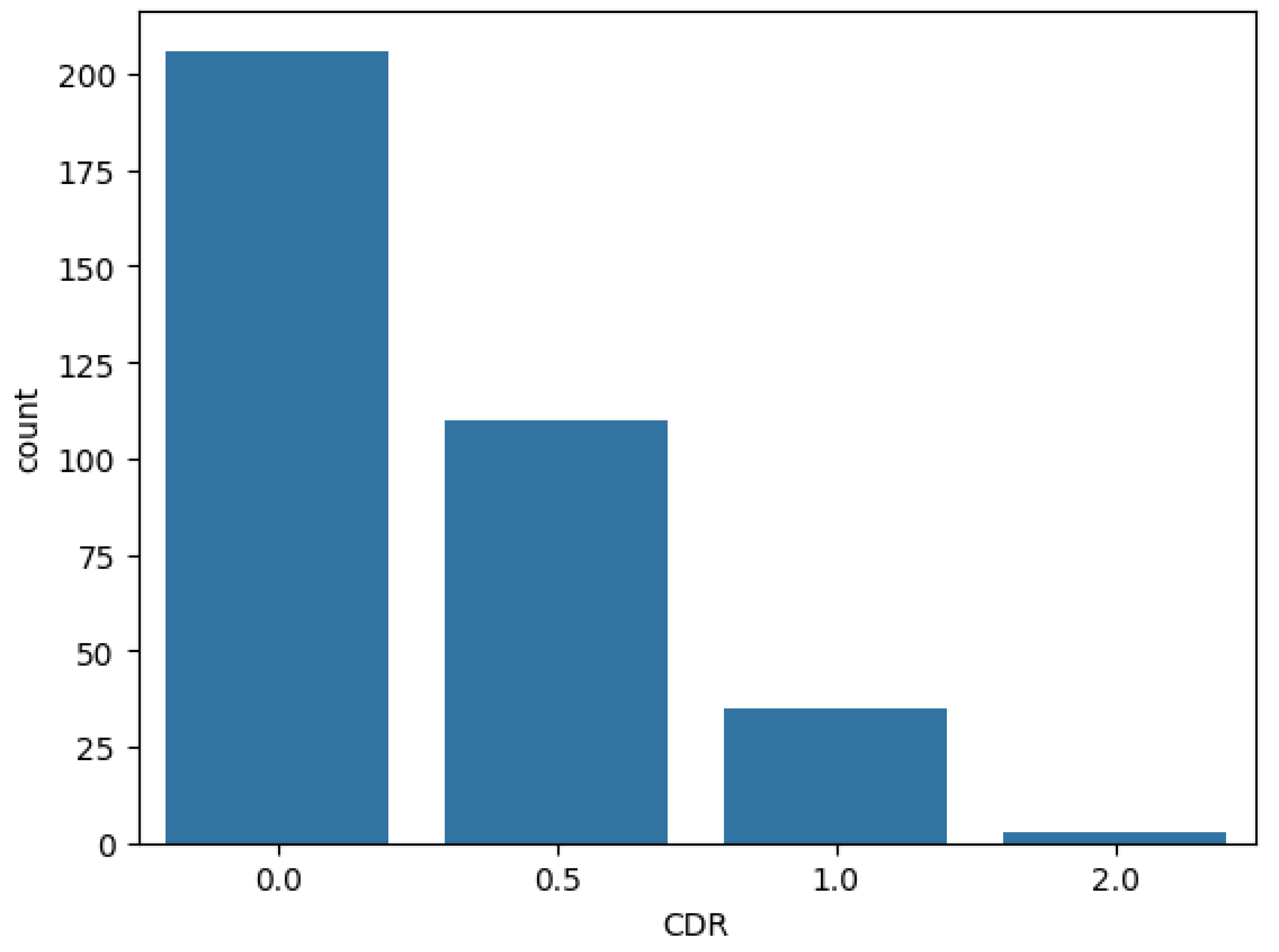
Figure 2.
CDR class distribution after preprocessing
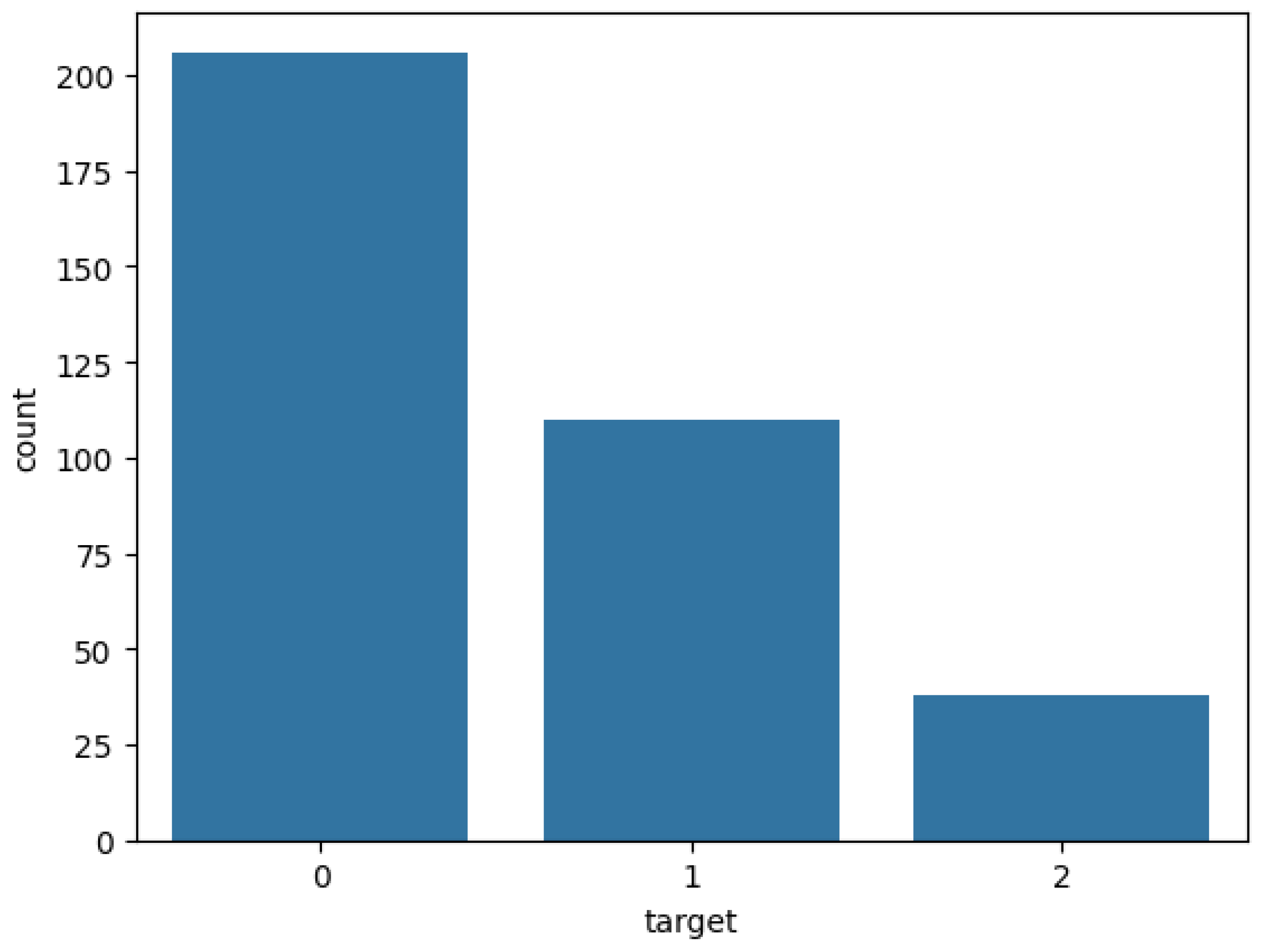
Figure 3.
Normalized Whole Brain Volume distribution
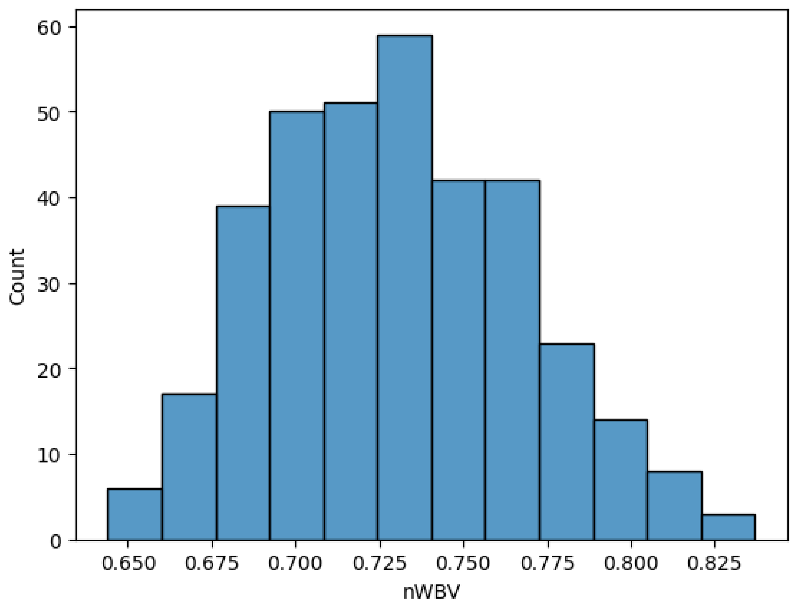
Figure 4.
MMSE Score distribution
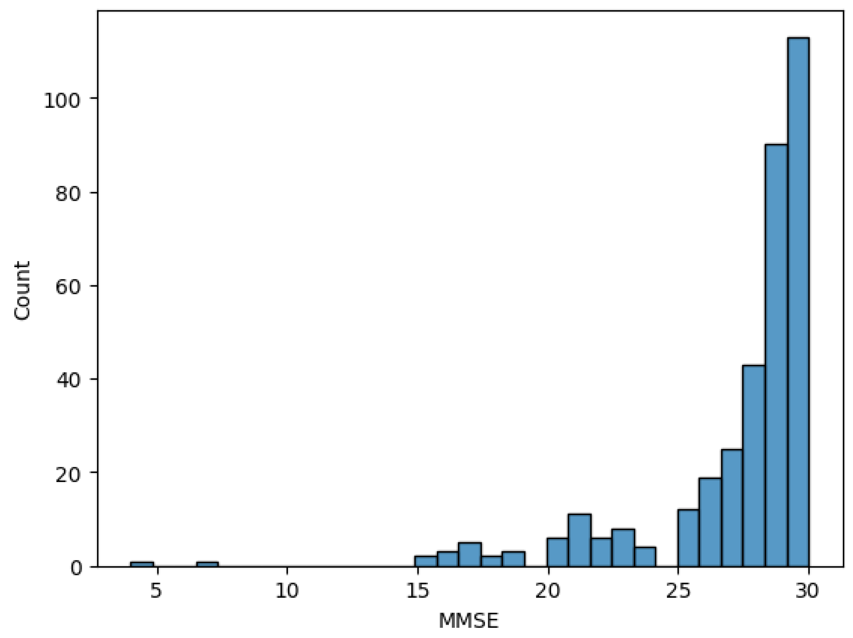
Figure 5.
Education level distribution
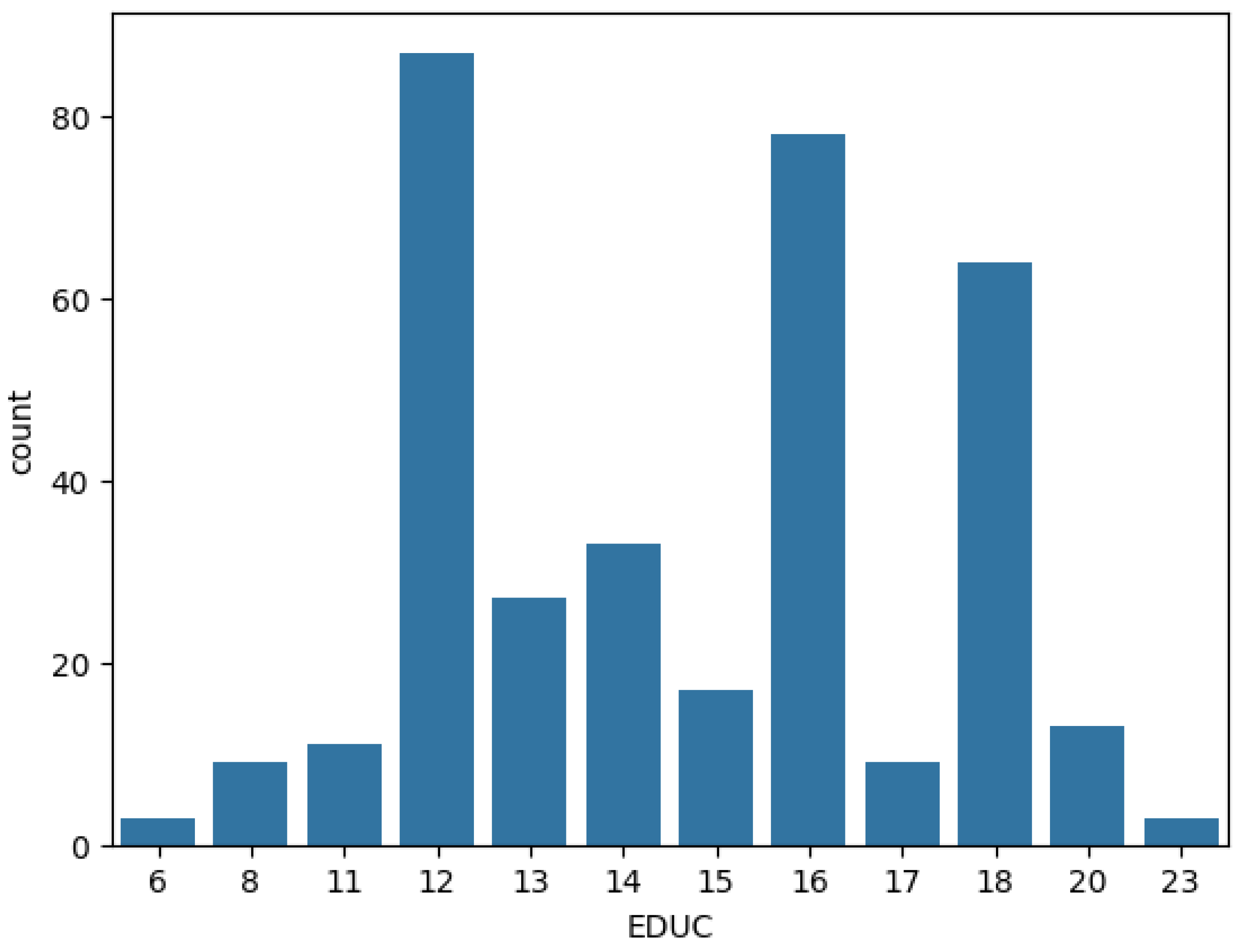
Figure 6.
SHAP values for class 0
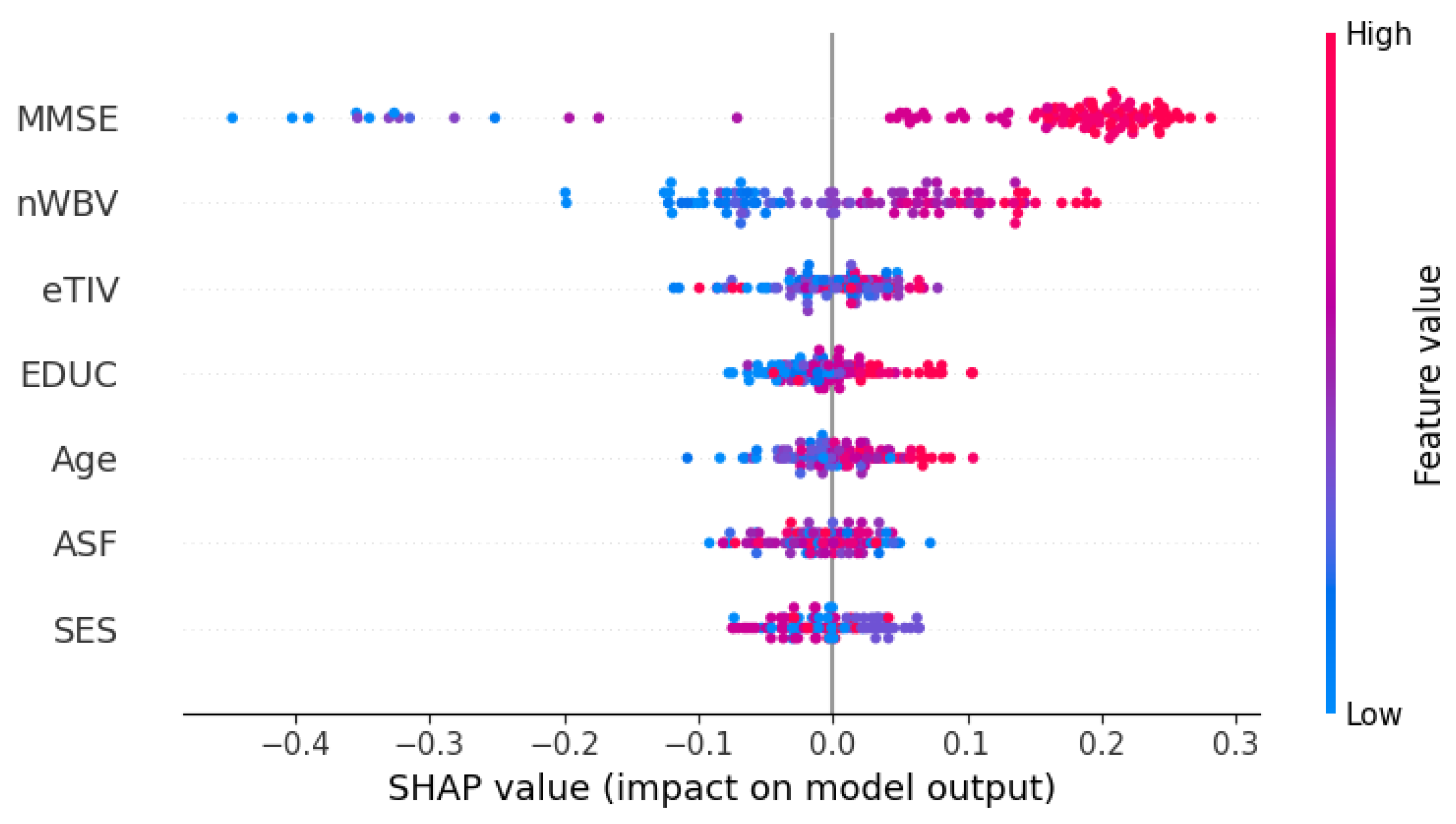
Figure 7.
SHAP values for class 1
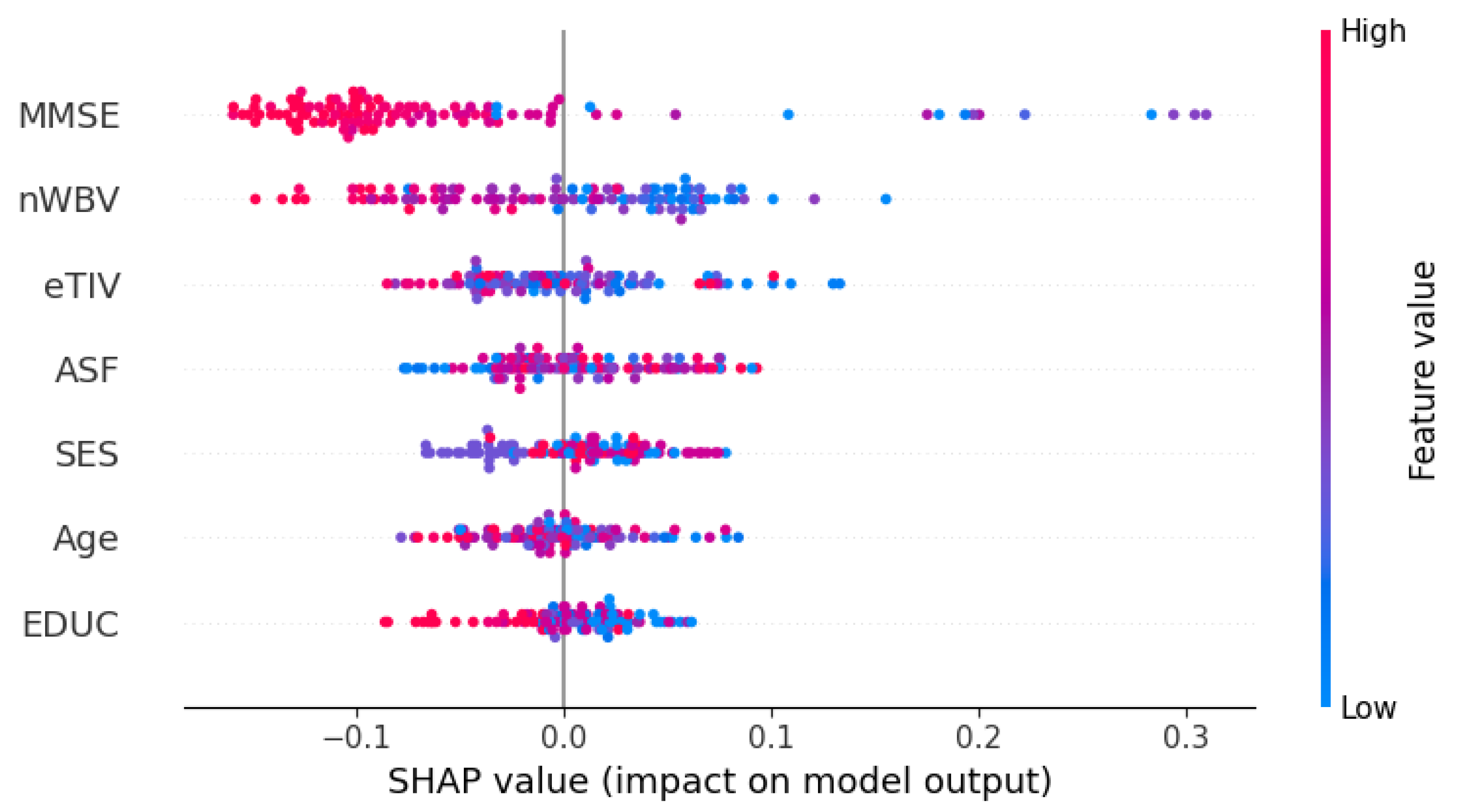
Figure 8.
SHAP values for class 2
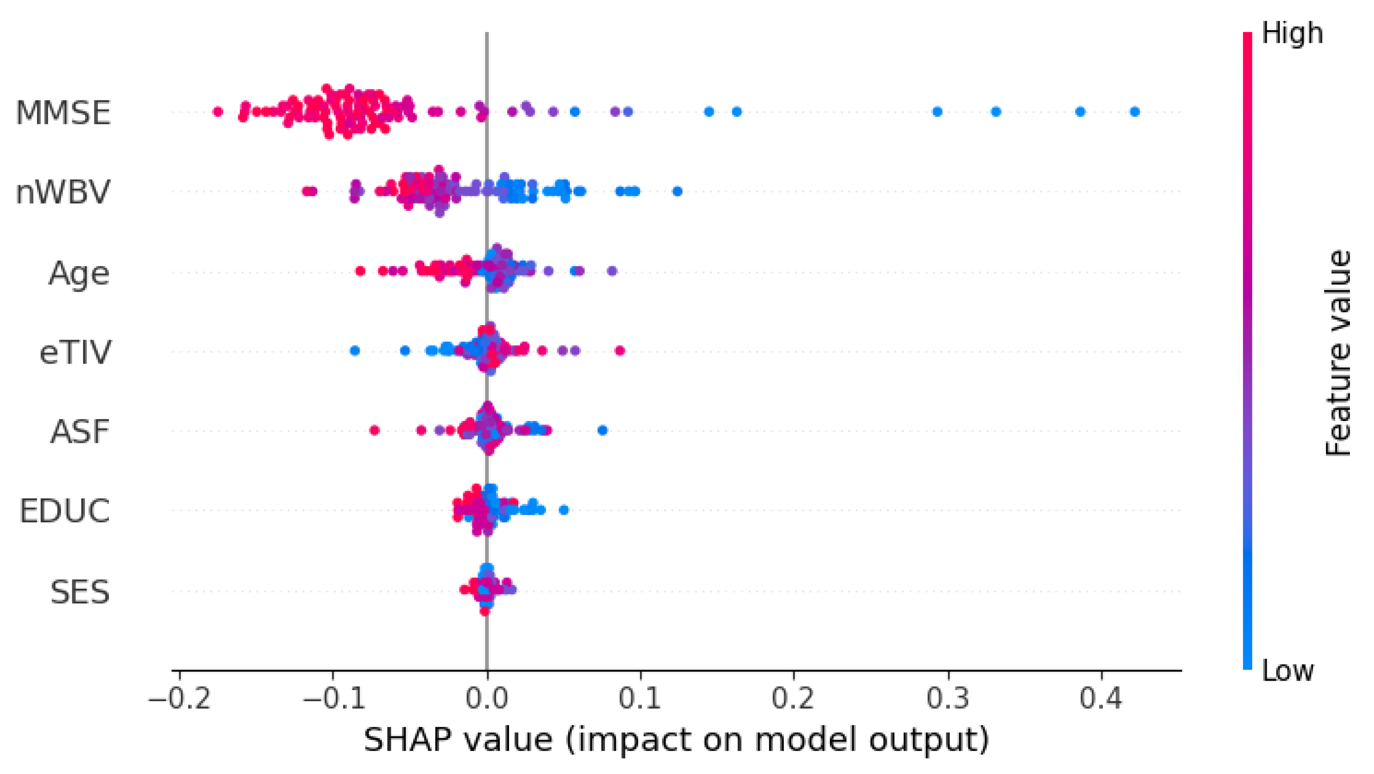

Table 1.
Caption describing the table contents.
| Abbreviation | Name of feature | Domain |
| Age | Age | Demographic & Socioeconomic |
| SES | Socioeconomic Status | |
| EDUC | Education | |
| nWBV | Normalized Whole Brain Volume | Neurobiological |
| eTIV | Estimated Total Intracranial Volume | |
| ASF | Atlas Scaling Factor | |
| MMSE | Mini-Mental State Exam score | Cognitive |
Table 2.
Classification performance report by class
| Precision | Recall | F1-Score | |||||||
|---|---|---|---|---|---|---|---|---|---|
| 0 | 1 | 2 | 0 | 1 | 2 | 0 | 1 | 2 | |
| All Domains | 0.91 | 0.83 | 1.00 | 0.99 | 0.73 | 0.57 | 0.95 | 0.78 | 0.73 |
| Demographic & Socioeconomic |
0.78 | 0.46 | 0.30 | 0.77 | 0.42 | 0.43 | 0.78 | 0.44 | 0.35 |
| Neurobiological | 0.80 | 0.70 | 0.56 | 0.91 | 0.52 | 0.50 | 0.85 | 0.59 | 0.53 |
| Cognitive | 0.74 | 0.67 | 0.86 | 0.94 | 0.50 | 0.78 | 0.89 | 0.57 | 0.75 |
Table 3.
Overall classification performance report
| Accuracy | Precision | Recall | F1-Score | ||||
|---|---|---|---|---|---|---|---|
| Macro | Weighted | Macro | Weighted | Macro | Weighted | ||
| All Domains | 0.90 | 0.91 | 0.90 | 0.76 | 0.90 | 0.82 | 0.89 |
| Demogprahic & Socioeconomic |
0.66 | 0.51 | 0.67 | 0.54 | 0.66 | 0.52 | 0.67 |
| Neurobiological | 0.76 | 0.68 | 0.75 | 0.64 | 0.76 | 0.66 | 0.75 |
| Cognitive | 0.80 | 0.79 | 0.79 | 0.70 | 0.80 | 0.74 | 0.79 |
Table 4.
Comparison of models’ performance by class
| Precision | Recall | F1-Score | |||||||
|---|---|---|---|---|---|---|---|---|---|
| 0 | 1 | 2 | 0 | 1 | 2 | 0 | 1 | 2 | |
| RF | 0.91 | 0.83 | 1.00 | 0.99 | 0.73 | 0.57 | 0.95 | 0.78 | 0.73 |
| SVM | 0.69 | 0.00 | 0.00 | 1.00 | 0.00 | 0.00 | 0.82 | 0.00 | 0.00 |
| kNN | 0.88 | 0.59 | 0.71 | 0.78 | 0.71 | 0.77 | 0.82 | 0.65 | 0.74 |
| XGBoost | 0.86 | 0.68 | 1.00 | 0.95 | 0.58 | 0.57 | 0.90 | 0.62 | 0.73 |
Table 5.
Comparison of models’ overall performance
| Accuracy | Precision | Recall | F1-Score | ||||
|---|---|---|---|---|---|---|---|
| Macro | Weighted | Macro | Weighted | Macro | Weighted | ||
| RF | 0.90 | 0.91 | 0.90 | 0.76 | 0.90 | 0.82 | 0.89 |
| SVM | 0.69 | 0.23 | 0.48 | 0.33 | 0.69 | 0.27 | 0.57 |
| kNN | 0.76 | 0.73 | 0.77 | 0.75 | 0.76 | 0.74 | 0.76 |
| XGBoost | 0.83 | 0.85 | 0.83 | 0.70 | 0.83 | 0.75 | 0.82 |
Disclaimer/Publisher’s Note: The statements, opinions and data contained in all publications are solely those of the individual author(s) and contributor(s) and not of MDPI and/or the editor(s). MDPI and/or the editor(s) disclaim responsibility for any injury to people or property resulting from any ideas, methods, instructions or products referred to in the content. |
© 2024 by the authors. Licensee MDPI, Basel, Switzerland. This article is an open access article distributed under the terms and conditions of the Creative Commons Attribution (CC BY) license (http://creativecommons.org/licenses/by/4.0/).
Copyright: This open access article is published under a Creative Commons CC BY 4.0 license, which permit the free download, distribution, and reuse, provided that the author and preprint are cited in any reuse.


