
Submitted:
08 January 2025
Posted:
09 January 2025
You are already at the latest version
Abstract
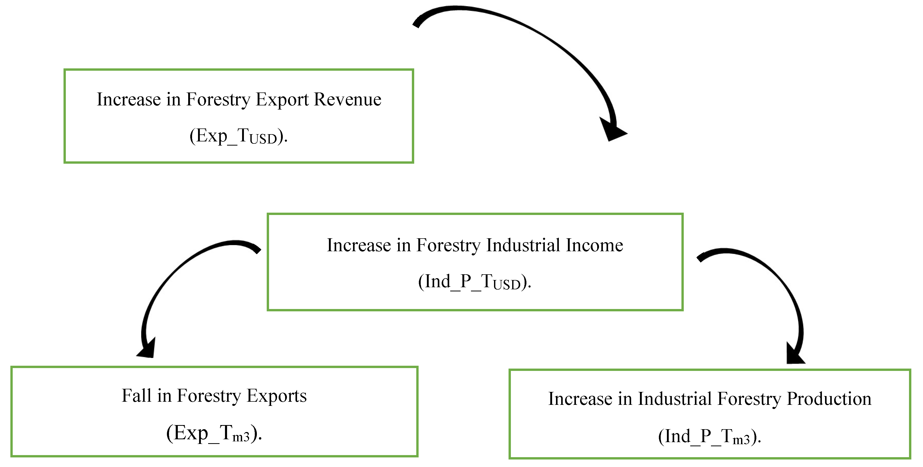
Gabon's decision to stop exports of forestry raw materials and to develop an industrialization strategy made it possible to apply certain theories of regional growth. The creation of the Nkok Special Economic Zone in 2012 (considered a homogeneous space unlike the external zone of the SEZ, considered heterogeneous) and the improvement of infrastructure illustrate the use of Rosenstein-Rodan's "Big push" theories and the Douglass North export base). These investments have fostered a process of unbalanced economic polarization, as theorists such as François Perroux have studied. Thanks to the use of the “Bias-Corrected Estimation of linear dynamic panel data” model, the analysis of industrial and commercial relationships and mechanisms during the period 2014-2022 show that the homogeneous space has positively influenced the heterogeneous space and the macroenvironment. This led to an increase in industrial income linked to exports, except for forestry products due to the ban on the export of raw materials. Export revenues boosted industrial production, while an increase in industrial revenues led to a decline in raw material exports, favoring domestic processing. The study makes it possible, using data from short and unbalanced panels, to carry out suitable estimation methods by establishing a decision-making process which results in an optimal model to be used for modeling spatial imbalance. This polarization process needs to be further studied to understand long-term economic and geographic imbalances in developing countries.
Keywords:
Introduction
I. Literature Review
I.1. Theoretical Foundations of Polarization and Associated Phenomena
I.1.1. Theories of Balanced Regional Growth
I.1.1.1. The Big Push Theory
I.1.1.2. “Export Base” Theories
I.1.2. The Theory of Unbalanced Regional Growth
I.1.2.1. The Theory of Growth Poles
I.1.2.2. The Theory of Cumulative Circular Causation
I.1.2.3. Hirschman's Theories of Unbalanced Growth
I.2. Contextual Frameworks of the Economic and Geographical Spaces Studied
I.2.1. Presentation of the Nkok Special Economic Zone
I.2.1.1. Creation of the Nkok Special Economic Zone
I.2.1.2. Attractive Tax Regime for Multinational Firms
- “Investors, companies affiliated to the Nkok SEZ and their subcontractors are exempt from obtaining the necessary permits and authorizations for the constructions and installations that they carry out in application of their investment program if the latter has been expressly approved by the planning and management body and endorsed by the administrative authority”.
- “The products manufactured and services provided by companies admitted to the Nkok SEZ regime are intended, for at least 75%, for export”.
- “The products manufactured and services provided by admitted companies may be sold on the national market, up to a maximum of 25% of their total production and/or services”.
- “The exemption from withholding tax, valid when at the end of twenty-five years following the first sale of the company, concerns in particular the 10% withholding on payments for the benefit of non-resident service providers and permanent establishments established in Gabon and belonging to a capital company whose head office is abroad”. (Journal O. RP. G, 2011) [12].
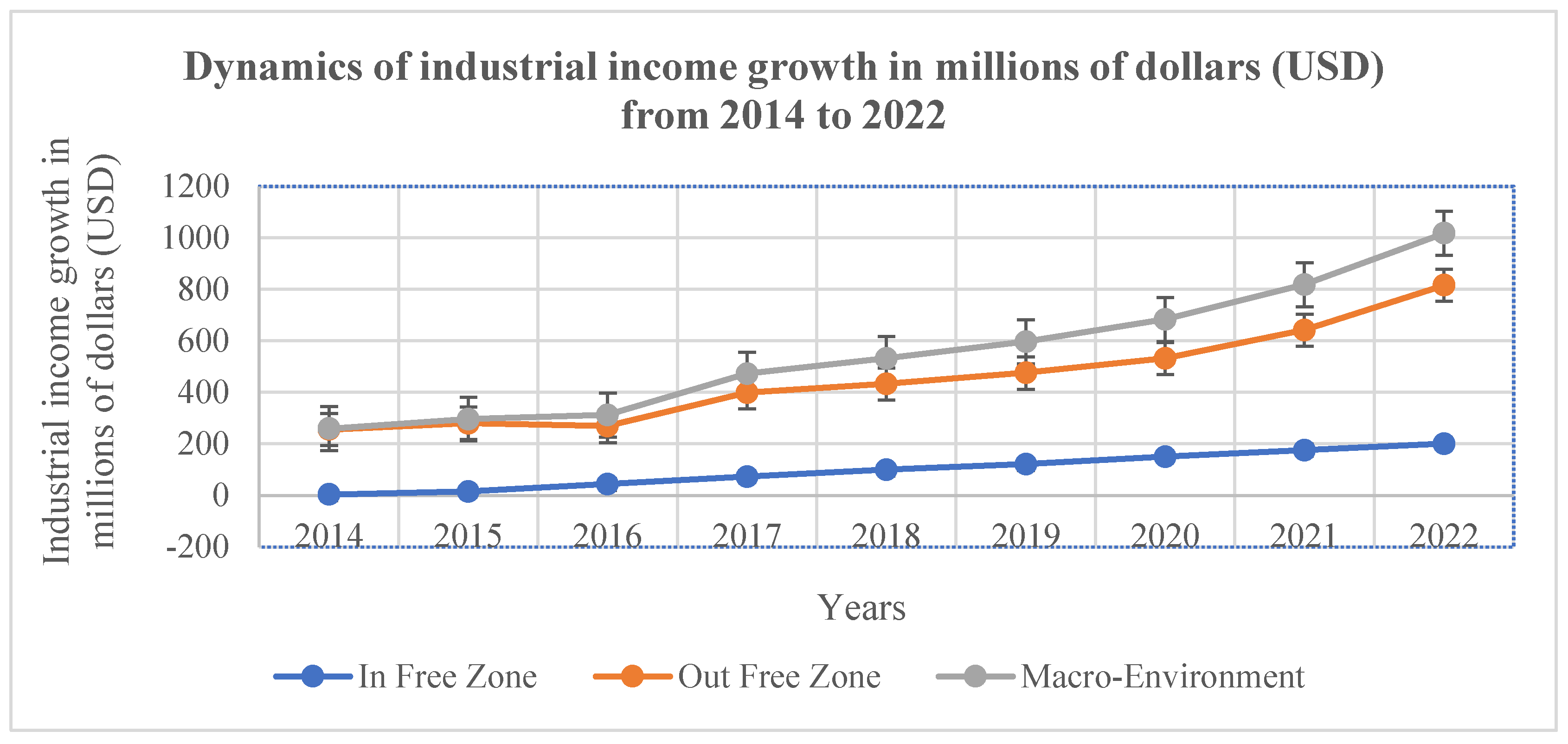
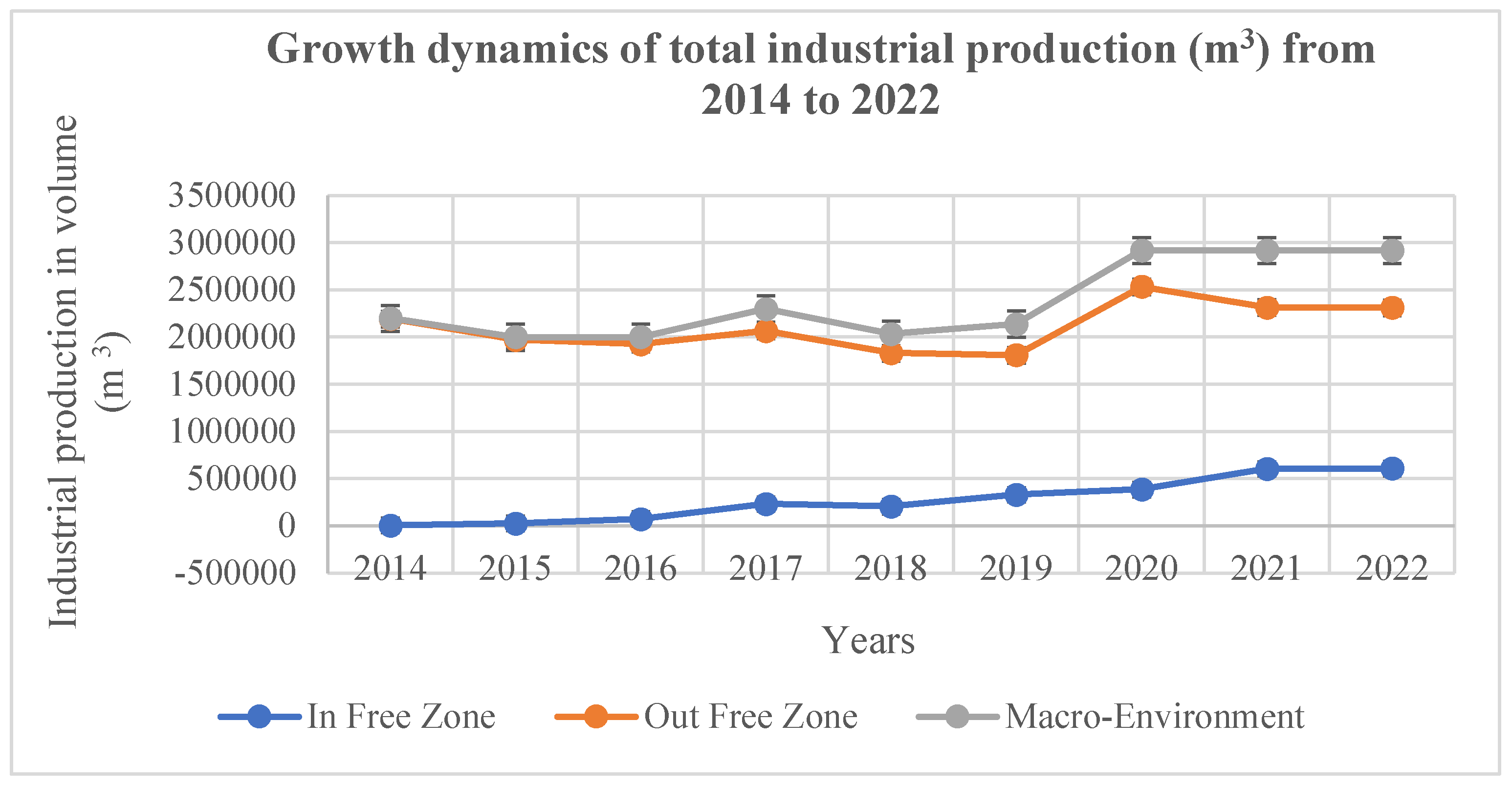
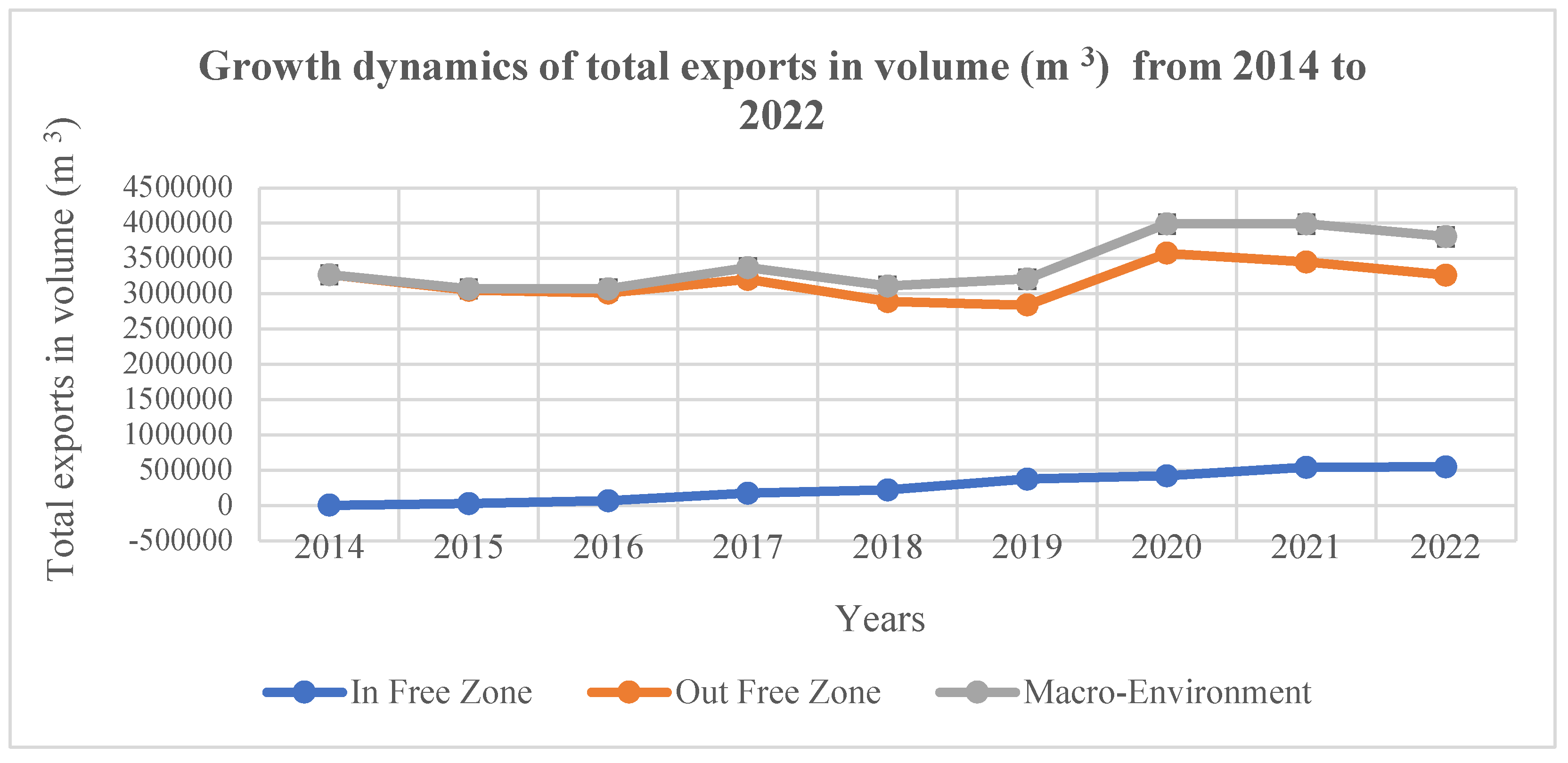
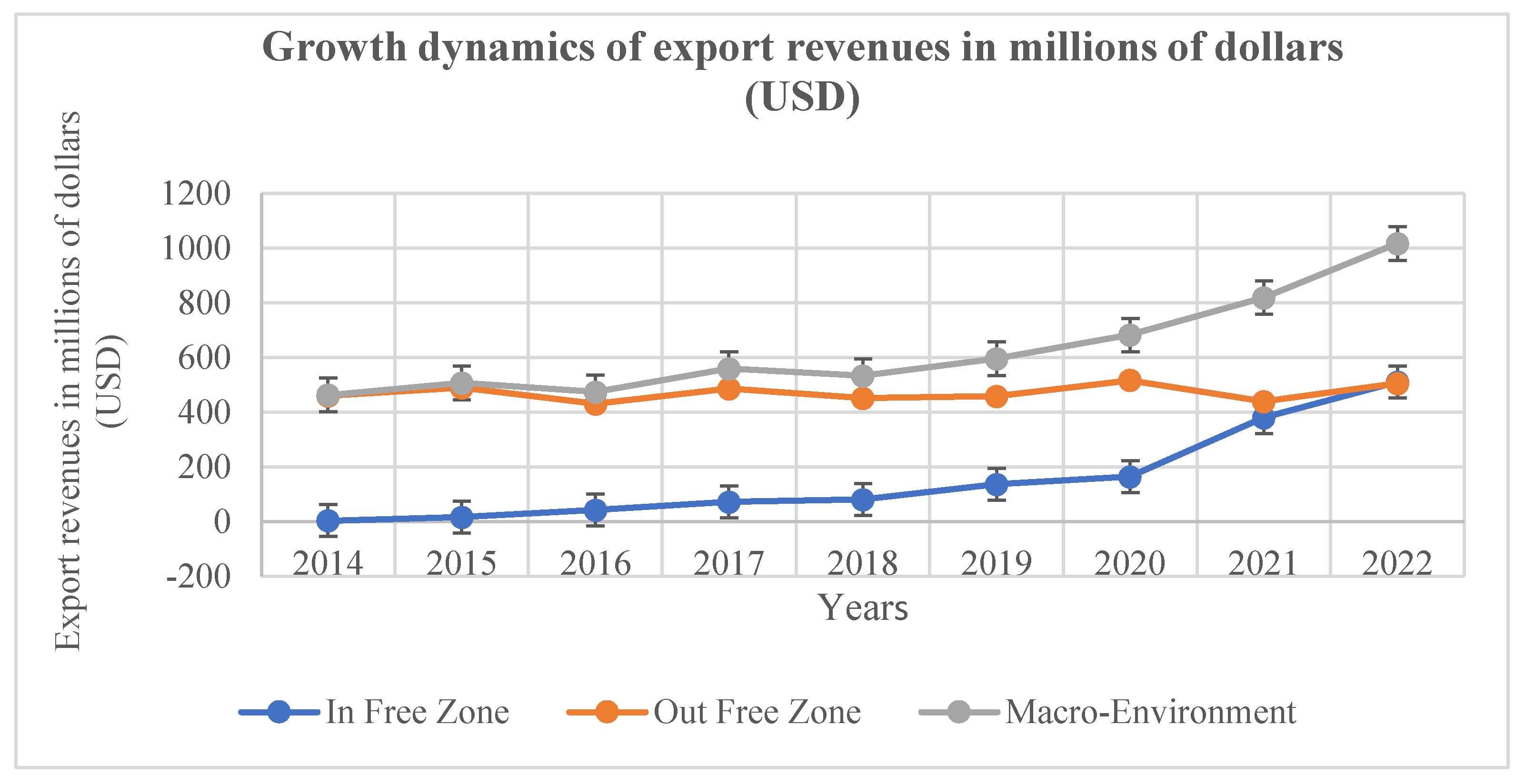
II.2. Production Volume and Industrial Income in Polarized Spaces
II. Methodology
II.1. Data Sources
- The first model makes it possible to carry out static and dynamic panel estimates with N =2 and T=9. The results of these estimations make it possible to study the effects of the “In Free Zone” space on the “Macroenvironment” space;
- The second model makes it possible to carry out static and dynamic panel estimates with N =2 and T=9. The results of these estimations make it possible to study the effects of the “Out Free Zones” space on the “Macroenvironment” space;
- The third model makes it possible to carry out static and dynamic panel estimates with N =3 and T=9. The results of these estimations make it possible to study the simultaneous effects of “In Free Zone” and “Out Free Zones” spaces on the “Macroenvironment” space.
II.2. Deterministic Macroeconomic Functions
- The total industrial income in values is obtained by subtracting the total income from the non-industrial income. That's to say :
- Regarding production in volume, we obtain:
II.3. Stochastic Modeling
II.3.1. Managing the Problem of Estimation Bias
- Low sample N estimation methods, which are non-parametric and robust estimation methods but have low power compared to parametric estimation methods, help to correct the biases linked to the size N;
- Estimation methods to resolve biases linked to the weakness of the temporal dimension are presented for the first time by Nickell (1981) [13]. And since then, methods such as GMM methods have made it possible to solve these problems. As part of this study, new estimation methods to resolve estimation biases will be used. Methods such as Arellano-Brover & Blundell-Bond, One-step system GMM and FE-Bias-Corrected Estimation.
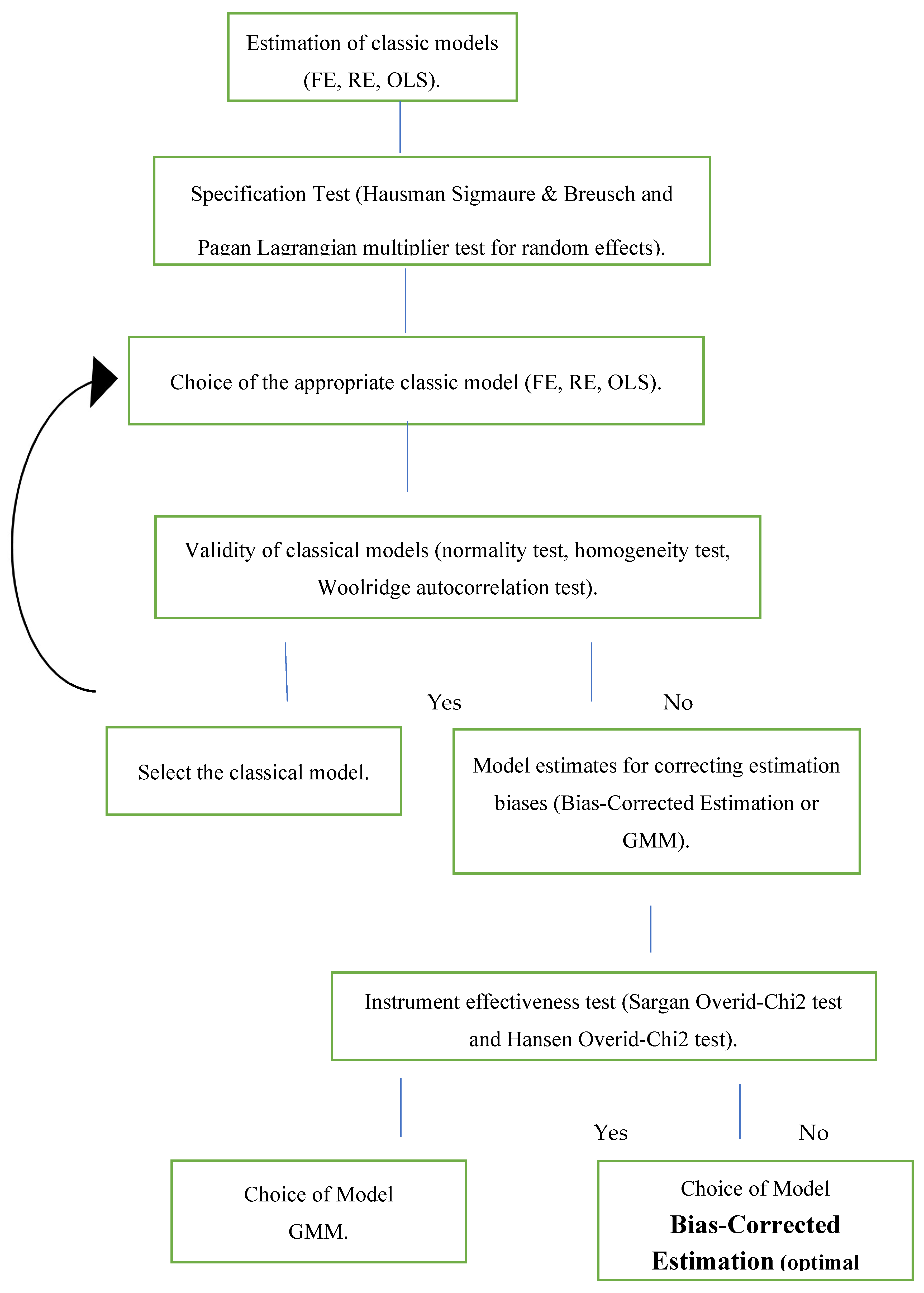
- Finally, the use of numerous estimates to understand and apprehend estimation biases is of great use for this study. However, a decision-making process for choosing the optimal model must be used for the study of each geographical space in order to obtain guidelines for public and private policies at the scale of the sector and at the macroeconomic level.
- Normality tests (Jarque-Bera normality test),
- Homoscedasticity tests (Breusch–Pagan/Cook–Weisberg test for heteroskedasticity (White))
- Autocorrelation tests (Wooldridge test for autocorrelation)
II.3.2. Correct Estimation of Biased Linear Dynamic Panel Data Model
II.3.1.1. General Form of Linear Dynamic Panel Data Model
- The minimum individual and temporal dimensions are N=2 and T=2, they can extend to infinity (Breitung, Kripfganz, and Hayakawa, 2021) [15].
- The autoregressive (higher order) model with P lags of the dependent variable and only minimal regularity conditions on the initial observations;
- Strictly exogenous xit repressors with respect to the idiosyncratic error term are:
- For Fixed Effects specific and random to unobserved groups,
- Serially Uncorrelated Idiosyncratic Errors are as follows:
III. Results and Discussions
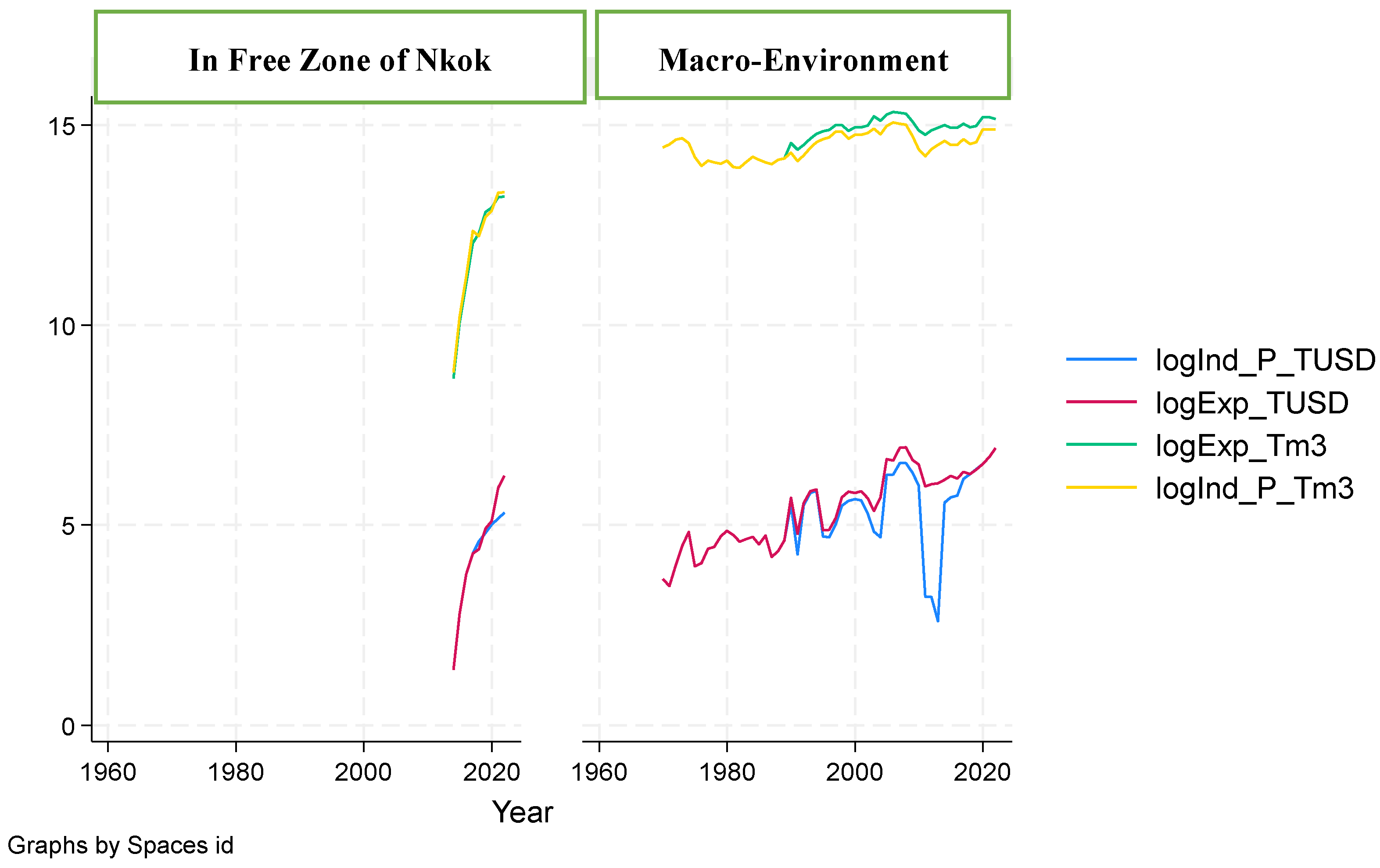
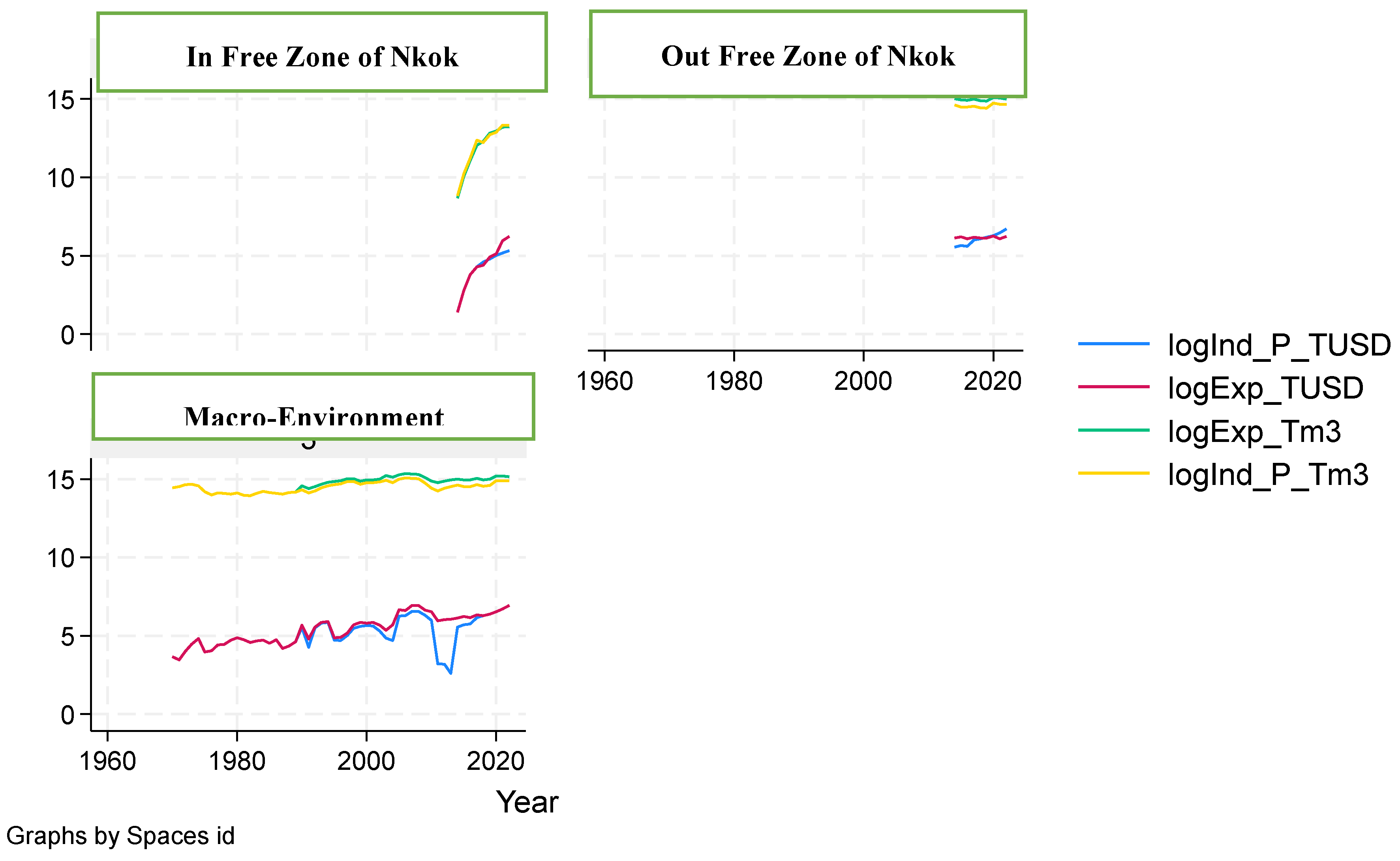
III.1. Descriptive Statistics
III.2. Classic Estimations

| (1) | (2) | (3) | |||
|---|---|---|---|---|---|
| Variables (In Free Zone) | OLS | Random Effect | Fixed Effect | ||
| LogInd_P_TUSD | |||||
| LogExp_TUSD | 0.99*** | 0.99*** | 1.12*** | ||
| (0.12) | (0.12) | (0.16) | |||
| LogExp_Tm3 | -2.11*** | -2.11*** | -2.55*** | ||
| (0.60) | (0.60) | (0.71) | |||
| LogInd_P_Tm3 | 2.24*** | 2.24*** | 2.49*** | ||
| (0.62) | (0.62) | (0.65) | |||
| Constant | -1.80 | -1.80 | 0.37 | ||
| (1.11) | (1.11) | (2.14) | |||
| (N/T) | 2/62 | 2/62 | 2/62 | ||
| Statistics | 51.87 | 155.60 | 45.69 | ||
| Test > f | 0.0000 | 0.0000 | 0.0000 | ||
| Corr (u_i, X or Xb) | 0 | 0.1475 | |||
| On R-squared | 0.7285 | 0.7285 | 0.7285 | ||
| (1) | (2) | (3) | |||
| Variables (Out Free Zone) | OLS | Random Effect | Fixed Effect | ||
| LogInd_P_TUSD | |||||
| LogExp_TUSD | 1.27*** | 1.27*** | 1.33*** | ||
| (0.17) | (0.17) | (0.15) | |||
| LogExp_Tm3 | -3.01*** | -3.01*** | -4.12*** | ||
| (0.77) | (0.77) | (0.74) | |||
| LogInd_P_Tm3 | 3.17*** | 3.17*** | 4.38*** | ||
| (0.78) | (0.78) | (0.76) | |||
| Constant | -3.51 | -3.51 | -4.96 | ||
| (4.27) | (4.27) | (3.81) | |||
| (N/T) | 2/62 | 2/62 | 2/62 | ||
| Statistics | 39.21 | 117.64 | 46.42 | ||
| Test > f | 0.0000 | 0.0000 | 0.0000 | ||
| Corr (u_i, X or Xb) | 0 | 0.0434 | |||
| On R-squared | 0.6698 | 0.6698 | 0.6484 | ||
| (1) | (2) | (3) | |||
| Variables (Macro-Environment) | OLS | Random Effect | Fixed Effect | ||
| LogInd_P_TUSD | |||||
| LogExp_TUSD | 0.98*** | 0.98*** | 1.12*** | ||
| (0.12) | (0.12) | (0.15) | |||
| LogExp_Tm3 | -1.47** | -1.47*** | -2.59*** | ||
| (0.56) | (0.56) | (0.67) | |||
| LogInd_P_Tm3 | 1.58*** | 1.58*** | 2.52*** | ||
| (0.58) | (0.58) | (0.62) | |||
| Constant | -1.37 | -1.37 | 0.45 | ||
| (1.12) | (1.12) | (2.05) | |||
| (N/T) | 3/71 | 3/71 | 3/71 | ||
| Statistics | 56.15 | 168.46 | 49.96 | ||
| Test > f | 0.0000 | 0.0000 | 0.0000 | ||
| Corr (u_i, X or Xb) | 0 | 0.1861 | |||
| On R-squared | 0.7155 | 0.7155 | 0.6686 | ||
III.3. Classic Specification and Validity test (OLS, RE and FE)
- Classic Spécification test
- Heteroskedasticity test
- Normality test
- Wooldridge autocorrélations test
III.4. Decision-Making Processes and Choice of the Optimal Model
III.5. Estimates With Error Corrected
III.5.1. Effects of the Nkok Special Economic Zone on the Macroenvironment
| (1) | (2) | (3) | (4) | |
|---|---|---|---|---|
| variables | Alejano Brover Brendel Bond |
GMM one-step system | One step system GMM-(robust) | FE-Bias-Corrected Estimation (robust) |
| LogInd_P_TUSD | ||||
| Δ*LogInd_P_TUSD | 0.35*** | 0.37*** | 0.37*** | 0.40*** |
| (0.06) | (0.08) | (0.03) | (0.05) | |
| LogExp_TUSD | 0.79*** | 0.74*** | 0.74*** | 0.83*** |
| (0.09) | (0.11) | (0.27) | (0.21) | |
| LogExp_Tm3 | -2.18*** | -1.91*** | -1.91 | -2.24* |
| (0.37) | (0.48) | (1.40) | (1.17) | |
| LogInd_P_Tm3 | 2.16*** | 1.96*** | 1.96 | 2.06 |
| (0.38) | (0.51) | (1.47) | (1.32) | |
| Constant | -0.16 | -1.07 | -1.07 | 1.52 |
| (1.14) | (1.12) | (2.12) | (2.70) | |
| Sargan test of overid-chi2 | 80.80 (0.013) | 80.80 (0.013) | ||
| Hansen test of overid-chi2 | 0.00 (1.000) | |||
| Autocorrelation order 1 Autocorrelation order 2 |
-1.1106 (0.2667) 1.0356 (0.3004) |
|||
| (N/T) | 60/2 | 60/2 | 60/2 | 60/2 |
| Ward Chi 2 (4) | 330.66 | 8196.39 | 302.07 | |
| p. value | 0.0000 | 0.000 | 0.000 |
III.5.2. Effects of the Region Outside the Nkok SEZ on the Macroenvironment
| (1) | (2) | (3) | (4) | |
|---|---|---|---|---|
| Variables | Alejano Brover Brendel Bond |
GMM one-step system | One step system GMM-(robust) |
FE-Bias-Corrected Estimation (robust) |
| LogInd_P_TUSD | ||||
| Δ*LogInd_P_TUSD | 0.39*** | 0.43*** | 0.43*** | 0.36*** |
| (0.05) | (0.07) | (0.09) | (0.02) | |
| LogExp_TUSD | 0.99*** | 0.92*** | 0.92*** | 1.02*** |
| (0.11) | (0.14) | (0.12) | (0.02) | |
| LogExp_Tm3 | -3.19*** | -2.65*** | -2.65*** | -3.55*** |
| (0.42) | (0.56) | (0.86) | (0.09) | |
| LogInd_P_Tm3 | 3.40*** | 2.80*** | 2.80*** | 3.77*** |
| (0.42) | (0.56) | (0.93) | (0.11) | |
| Constant | -4.51** | -3.62 | -3.62*** | -4.77*** |
| (2.23) | (3.06) | (1.14) | (0.33) | |
| Sargan test of overid-chi2 | 83.05 (0.009) | 83.05 (0.009) | ||
| Hansen test of overid-chi2 | 0.00 (1.000) | |||
| Autocorrelation order 1 Autocorrelation order 2 |
-1.0636 (0.2875) 1.0356 (0.3030) |
|||
| (N/T) | 60/2 | 60/2 | 60/2 | 60/2 |
| Ward Chi 2 (4) | 453.99 | 9885.60 | 10.04 | |
| p. value | 0.0000 | 0.000 | 0.040 | |
III.5.3. Effects of Industrial Income on Macro-Environmental Variables
| (1) | (2) | (3) | (4) | |
|---|---|---|---|---|
| Variables | Alejano Brover Brendel Bond |
GMM one-step system | One step system GMM--(robust) |
FE-Bias-Corrected Estimation (robust) |
| LogInd_P_TUSD | ||||
| Δ*LogInd_P_TUSD | 0.37*** | 0.44*** | 0.44*** | 0.412*** |
| (0.06) | (0.08) | (0.07) | (0.064) | |
| LogExp_TUSD | 0.81*** | 0.68*** | 0.68*** | 0.824*** |
| (0.08) | (0.11) | (0.26) | (0.216) | |
| LogExp_Tm3 | -2.12*** | -1.39*** | -1.39 | -2.244** |
| (0.34) | (0.44) | (1.39) | (1.134) | |
| LogInd_P_Tm3 | 2.05*** | 1.38*** | 1.38 | 2.065 |
| (0.35) | (0.46) | (1.47) | (1.285) | |
| Constant | 0.21 | -0.40 | -0.40 | 1.579 |
| (1.10) | (1.08) | (2.06) | (2.752) | |
| Sargan test of overid-chi2 | 92.58 (0.009) | 92.58 (0.009) | ||
| Hansen test of overid-chi2 | 0.00 (1.000) | |||
| Autocorrelation order 1 Autocorrelation order 2 |
-1.1420 (0.2534) 1.0467 (0.2952) |
|||
| (N/T) | 60/2 | 60/2 | 60/2 | 60/2 |
| Ward Chi 2 (4) | 366.66 | 9920.87 | 176.21 | |
| p. value | 0.0000 | 0.000 | 0.000 | |
III.6. Causality Tests
| Granger causality Tests | |||||
|---|---|---|---|---|---|
| Causality | Z-bar | p-value | Z-bar tilde | p-value | Remarks |
| Ind_P_TUSD- Exp_TUSD | 17,541 | 0.1360 | 13,450 | 0.0794 | Exp_TUSD does Granger-cause Ind_P_TUSD for at least one panel |
| Exp_TUSD-Ind_P_TUSD | 15,807 | 0.6479 | 0.4636 | 0.1140 | |
| Ind_P_TUSD-Exp_Tm3 | 0.9619 | 0.3361 | 0.8538 | 0.3932 | Ind_P_TUSD does Granger-cause Exp_Tm3 for at least one panel |
| Exp_Tm3-Ind_P_TUSD | 25,485 | 0.0108 | 23,273 | 0.0199 | |
| Ind_P_TUSD-Ind_P_Tm3 | 0.8259 | 0.4089 | 0.7275 | 0.4669 | Ind_P_TUSD does Granger-cause Ind_P_Tm3 for at least one panel |
| Ind_P_Tm3-Ind_P_TUSD | 48,121 | 0.0000 | 44,296 | 0.0000 | |
Policies and recommendations:
- Create a network of SEZs spread across several strategic regions, including rural or less developed areas.
- Develop SEZs focused on local resources (e.g. agro-industry in agricultural regions).
- Connect SEZs through transport infrastructure to promote regional economic integration.
- Use revenues generated by SEZs to finance infrastructure in surrounding regions.
- Build roads, electricity networks and sanitation facilities connecting rural areas to SEZs.
- Promote integrated development programs to connect urban and rural areas.
- Encourage businesses located in SEZs to source from local suppliers.
- Provide incentives for SMEs to participate in the value chains of industries present in SEZs.
- Train and finance local businesses so that they can meet the required quality standards.
- Establish a mechanism for redistributing income generated by SEZs to less developed regions.
- Create regional development funds funded by part of the taxes or profits generated by the SEZs.
- Establish quotas or Investment obligations in local infrastructure.
- Establish vocational training centers near SEZs to train the local workforce.
- Include specific training programs for women and young people, who are often excluded from opportunities.
- Establish local hiring quotas in SEZs.
- Develop links between SEZs and regional economies (e.g. local agriculture to supply food industries).
- Create economic corridors connecting SEZs to peripheral regions to stimulate economic activity along these corridors.
- Promote co-development projects where several regions benefit from the same investment.
- Ensure equitable regional planning to distribute resources and investments.
- Strengthen transparency in the award of contracts, management of funds and assessment of the impacts of SEZs.
- Establish regional institutions to monitor the impact of SEZs on local communities.
- Integrate ecological practices in SEZs to protect the local environment.
- Implement social responsibility programs to support surrounding communities.
- Ensure public consultation with local populations before the implementation of new projects.
- Involve the private sector in the development of infrastructure outside SEZs.
- Promote PPPs to finance educational, health or economic projects in underdeveloped areas.
- Establish monitoring indicators to measure the economic, social and environmental impacts of SEZs.
- Readjust policies based on results to better meet regional needs.
- Involve local stakeholders in planning and evaluation processes.
Conclusions
Author Contributions
Funding
Informed Consent Statement
Data Availability Statement
Conflicts of Interest
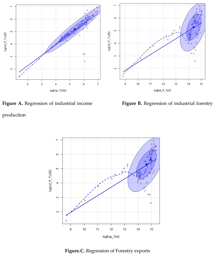
Appendix: Point Clouds in the Macroenvironment
References
- Perroux, F. Note on the notion of “growth pole”. Applied Economics 1955, 8, 307–320. [Google Scholar]
- Myrdal, G. Economic theory and underdeveloped areas; Duckworth: London, 1957. [Google Scholar]
- Hirschmann, A.O. Economic development strategy; Yale University Press: New Haven, 1958. [Google Scholar]
- Milton, S. Underdevelopment and poles of economic and social growth, Persée. In Tiers-Monde; 1974; Volume 15, pp. 271–286. [Google Scholar]
- Misra, R.P. Regional planning and national development, Goodreads ed.; Vikas Publishing: New Delhi, India, 1978; ISBN 10. [Google Scholar]
- Rosenstein-Rodan, P. The Problem of Industrialization of Eastern and South-Eastern Europe. The Economic Journal 1943, 53, 202–211. [Google Scholar] [CrossRef]
- Rosenstein-Rodan. The International Development of Economically Disadvantaged Regions. International Affairs 1944, 20, 157–65. [Google Scholar] [CrossRef]
- Nurkse, R. Causes and Effects of Capital Movements, Equilibrium and Growth in the World Economy. Economic Essays by Ragnar Nurkse, Cambridge; 1961; pp. 1–21. [Google Scholar]
- Isard, W. Location and spatial economy: general theories related to industrial location, market areas, land use, trade and urban structure; MIT Press: Cambridge, 1956. [Google Scholar]
- North, D.C. Institutions, Institutional Change and Economic Performance; Cambridge University Press: Cambridge, MA, USA, 1990; pp. 107–140. [Google Scholar]
- Jandir, F.L. Notes on growth poles and territorial strategies in Quebec. JF De Lima - Canadian Journal of Regional Science 2005, 2005. [Google Scholar]
- Official Journal of the Gabonese Republic. Decree No. 461/PR/MPITPTHTAT of October 10, 2012 establishing and organizing the NKOK Privileged Regime Economic Zone; 10 October 2012. [Google Scholar]
- Nickel, S. Deviations in dynamic models with fixed effects. Econometrics 1981, 49, 1417–1426. [Google Scholar] [CrossRef]
- Dhaene, G.; Jochmans, K. Likelihood reasoning in autoregression with fixed effects. Econometric Theory 2016, 32, 1178–1215. [Google Scholar] [CrossRef]
- Breitung, J.; Kripfganz, S.; Hayakawa, K. Offset correction method for moment estimator of dynamic panel data model. Econometrics and Statistics: The Future 2021. [Google Scholar]
- Bun, M.J.G.; Carree, M.A. Bias correction estimation in dynamic panel data model. Journal of Business and Economic Statistics 2005, 23, 200–210. [Google Scholar] [CrossRef]
- Kripfganz, S. Quasi-maximum likelihood estimation of linear dynamic short-T panel data models. Stata Journal 2016, 16, 1013–1038. [Google Scholar] [CrossRef]
- Kripfganz, S. A general method for moment estimation of linear dynamic panel data model. Minutes of London STATA Conference 2019: Application of Employment Equation. Economic Research Review 2019, 58, 277–297. [Google Scholar]
- Frick, S.A.; Rodriquez-Pose, A.; Wong, M.D. Towards economically dynamic special economic zones in emerging countries. Economic Geography 2019, 95, 30–64. [Google Scholar] [CrossRef]
- Moberg, L. The political economy of political economic zones. Journal of Institutional Economics 2015, 11, 167–190. [Google Scholar] [CrossRef]
- Tangtipongkul, K.; Srisuchart, S.; Nuchmon, N.; Vinayavekhin, S. Local economic development to support opportunities and impacts from special economic zones along the greater Mekong subregion southern economic corridor: Case studies in Kanchanaburi and trat provinces. Thammasat Review 2021, 24, 79–110. Available online: https://sc01.tci-thaijo.org/index.php/tureview/article/view/239905.
- Thombs, R.P. A Guide to Analyzing Large N, Large T Panel Data. Socius: Sociological Research for a Dynamic World 2022, 8, 1–15. [Google Scholar] [CrossRef]

| Variable | Stand points | Units | Describe |
|---|---|---|---|
| Ind_P_TUSD (Industrial Income) |
Variable Dependent |
Millions of dollars (USD) | Total industrial production in value (million USD), represents the total sum of industrial revenues of companies in the woody forestry sector on the territory of Gabon. Noted : Ind_P_TUSD. |
| Exp_TUSD (Export Income) |
Independent variable | Millions of dollars (USD) | Total exports in millions of USD dollars, represents the export income of Gabon's woody forest products. Noted : Exp_TUSD. |
| Exp_Tm3 (Forestry Exports) |
Independent variable | Cubic meter (m 3) | Total exports in m 3, which represents the national volume of exports of wood forest products from Gabon. Noted: Exp_Tm3. |
| Ind_P_Tm3 (Industrial Forestry Production) |
Independent variable | Cubic meter (m 3) | Total industrial production in m 3, represents the total sum of industrial production (processed and unprocessed) of companies in the woody forestry sector in Gabon. Noted: Ind_P_Tm3. |
| Source 1 : FAOSTAT : https://www.fao.org/faostat/en/#data/FO Source 2: Dashboard of the economy of Gabon: http://www.dgepf.ga/23-publications/25-table-de-bord-de-l-economie/169-table-de-bord-de-l-economie// | |||
| Variables | Parameters | Mean | STD. Dev. | Min | Max |
|---|---|---|---|---|---|
| Ind_P_TUSD | Amount to | 229.271 | 225.1.344 | 4 | 1018 |
| between | 108.209 | 98.454 | 251.485 | ||
| inside | 218.476 | -8.810 | 995.785 | ||
| Exp_TUSD | Amount to | 306.161 | 274.364 | 4 | 1036.298 |
| between | 123.591 | 156.749 | 331.5338 | ||
| inside | 267.250 | 6.828 | 1010.926 | ||
| Exp_Tm3 | Amount to | 2245464 | 1260365 | 5807.998 | 4570000 |
| between | 1640283 | 262484.9 | 2582196 | ||
| inside | 953855.2 | 798267.8 | 4233268 | ||
| Ind_P_Tm3 | Amount to | 1801760 | 885762.3 | 6798.346 | 3500000 |
| between | 1262967 | 274927.7 | 2061033 | ||
| inside | 618238 | 875726.6 | 3240727 |
| Variables | Parameters | Mean | STD. Dev. | Min | Max |
|---|---|---|---|---|---|
| Ind_P_TUSD | Amount to | 281.171 | 238.654 | 13.404 | 1018 |
| between | 144.606 | 251.485 | 455.9899 | ||
| inside | 227.334 | 43.901 | 1047.686 | ||
| Exp_TUSD | Amount to | 351.803 | 264.561 | 32.2 | 1036.298 |
| between | 987.367 | 331.533 | 471.1686 | ||
| inside | 259.872 | 52.469 | 1056.568 | ||
| Exp_Tm3 | Amount to | 2667292 | 977331.6 | 1135000 | 4570000 |
| between | 414520 | 2582196 | 3168416 | ||
| inside | 954900.1 | 1220096 | 4655096 | ||
| Ind_P_Tm3 | Amount to | 2067567 | 619458.5 | 1135000 | 3500000 |
| between | 31828.28 | 2061033 | 2106045 | ||
| inside | 619252.2 | 1141534 | 3506534 |
| Variables | Parameters | Mean | STD. Dev. | Min | Max |
|---|---|---|---|---|---|
| Ind_P_TUSD | Amount to | 258.01 | 232.255 | 4 | 1018 |
| between | 179.384 | 98.454 | 455.989 | ||
| inside | 213.536 | 19.928 | 1024.525 | ||
| Exp_TUSD | Amount to | 327.078 | 262.216 | 4 | 1036.298 |
| between | 157.536 | 156.7495 | 471.168 | ||
| inside | 249.685 | 27.744 | 1031.842 | ||
| Exp_Tm3 | Amount to | 2362457 | 1219393 | 5807.998 | 4570000 |
| between | 1536725 | 262484.9 | 3168416 | ||
| inside | 894348.8 | 915261.7 | 4350262 | ||
| Ind_P_Tm3 | Amount to | 1840331 | 837329.9 | 6798.346 | 3500000 |
| between | 1044445 | 274927.7 | 2106045 | ||
| inside | 583181.9 | 914298 | 3279298 |
| Housman test (Sigmaure) | |||
|---|---|---|---|
| Spaces | Statistics | p.value | Remark |
| In Fee Zone | 1.4 | 0.237 | Random Effect is appropriate |
| Out Free Zone | 13.02 | 0.0003 | Fixed Effect is appropriate. |
| Macro-Environment | 10 | 0.0067 | Fixed Effect is appropriate. |
| Breusch and Pagan Lagrangian multiply test | |||
| Song title: In Fee Zone | 0.00 | 1.00 | Pooled Model is Adaptive pool model is suitable. |
| Breusch – Pagan/Book – Weisberg heterogeneity test (white) | |||
|---|---|---|---|
| Spaces | Statistics | p.value | Remark |
| In Fee Zone | 2.03 | 0.1538 | Constant variance (Homoscedastic Residuals) |
| Out Free Zone | 2.39 | 0.1538 | Constant variance (Homoscedastic Residuals) |
| Macro-Environment | 1.05 | 0.3066 | Constant variance (Homoscedastic Residuals) |
| Jarque-Bera normality test | ||||
|---|---|---|---|---|
| Spaces | Statistics | p.value | Remark | |
| In Fee Zone | 120 | 8.60E-27 | Residue does not follow normal distribution | |
| Out Free Zone | 70.4 | 5.20E-16 | Residue does not follow normal distribution | |
| Macro-Environment | 92 | 1.10E-20 | Residue does not follow normal distribution | |
| Wooldridge autocorrelation test | |||
|---|---|---|---|
| Spaces | Statistics | p.value | Remark |
| In Fee Zone | 353.966 | 0.0338 | First order autocorrelation |
| Out Free Zone | 2613.494 | 0.0125 | First order autocorrelation |
| Macro-Environment | 271.794 | 0.0037 | First order autocorrelation |
Disclaimer/Publisher’s Note: The statements, opinions and data contained in all publications are solely those of the individual author(s) and contributor(s) and not of MDPI and/or the editor(s). MDPI and/or the editor(s) disclaim responsibility for any injury to people or property resulting from any ideas, methods, instructions or products referred to in the content. |
© 2025 by the authors. Licensee MDPI, Basel, Switzerland. This article is an open access article distributed under the terms and conditions of the Creative Commons Attribution (CC BY) license (http://creativecommons.org/licenses/by/4.0/).


