
Submitted:
08 January 2025
Posted:
08 January 2025
You are already at the latest version
Abstract
Industrially applied bioelectrochemical systems require for long-term stable operation and hence a control of the biofilm accumulation on the electrodes. An optimized application of biofilm control mechanisms presupposes an on-line, in-situ monitoring of the accumulated biofilm. Heat-transfer sensors have successfully been integrated into industrial systems for the on-line non-invasive monitoring of biofilms. In this study, a mathematical model for the description of the sensitivity of a heat-transfer biofilm sensor has been developed, incorporating the hydrodynamic conditions of the fluid and the geometrical properties of the substratum. This model was experimentally validated at different flow velocities by integrating biofilm sensors into cylindrical pipes and planar mesofluidic flow cells with a carbonaceous substratum. Dimensionless sensor readings were correlated with the mean biovolume measured gravimetrically and using optical coherence tomography to determine the sensor sensitivity. The biofilms sensors applied in the planar flow cells revealed an increase in sensitivity by a factor of 6 compared to standard stainless-steel pipes, as well as an improved sensitivity at higher flow velocities.
Keywords:
heat-transfer
; biofilm sensor
; hydrodynamics
; bioelectochemical system
; mathematical model
1. Introduction
The field of applications for bioelectrochemical systems (BES) is wide, utilizing various substrates/waste streams to produce value-added products, including energy efficient waste water treatment[1] with the use of microbial fuel cells (MFC) or the production of hydrogen in microbial electrolysis cells (MEC)[2]. Common denominator among BES are electroactive biofilms growing on the anode coupling the metabolic conversion of organic substrates by the anodic bacteria with extracellular electron transfer (EET) to a solid electrode. The morphology of the electroactive biofilm on the anode is of central importance to the efficiency and functionality of BES[3,4]. The goal of upscaling BES faces a number of challenges in the transition of laboratory sized reactors to pilot or industrial scale systems[5,6], among which is the efficient mass transfer between the bulk phase and the electroactive biofilm at the electrode-biofilm interface. In detail in a MFC organic carbon diffuses towards the anode where it is oxidized by the electroactive bacteria to CO2 and H+. The products need to diffuse out of the biofilm to the bulk phase. Otherwise, subsequent substrate gradients[7]–[9] or acidic pH environments[8,10] in the biofilm can limit or inhibit the electroactive bacteria in their current production. An additional bottleneck of transport phenomena, additionally hampering the anodic efficiency of BES, is the reported limited distance of the electron transfer from bacteria to electrode, by cytochromes, electron shuttles/mediators, or conductive pili[11]–[13]. The combination of limitations deriving from extracellular electron transfer distance and diffusion resistance along with the need for a high quantity of electroactive bacteria suggests an optimal biofilm thickness range for electroactive biofilms. Recent reported optimal biofilm thicknesses for electroactive model organisms range from a few µm for Shewanella sp.[14], approx. 10 µm (Desulfuromonas acetexigens[15]) up to 20-100 µm for Geobacter sulfurreducens[3,16,17].
With the aim of long-term stable bioelectrochemical processes in reactor systems utilizing waste streams a control of the biofilm thickness to the optimum range would support more efficient applications[18]. Therefore, a continuous monitoring of the state of the electroactive biofilm by means of on-line sensors on the anodes is desirable towards an industrially usable process control. Industrial applicable biofilm sensors require an on-line, in-situ and non-invasive characterization of the biofilm to provide relevant information of the biofilm morphology[19]. While most of the reported methods of biofilm monitoring have been investigated in lab-scale application, a few industrial applicable sensors including electrochemical sensors (e.g., ALVIM[20], BioGeorge[21], BIOX[22]), mechanical sensors (Solenis OnGuard[23]), optical (OPTIQUAD[24]) and thermal (DEPOSENS®[25,26]) are known. An extensive discussion of the advantages and limitations of the respective biofilm sensors or sensing methods can be found in the reviews by Janknecht and Melo[27], Nivens et al.[28] or Pereira and Melo[19].
Thermal biofilm sensors, utilizing the additional thermal resistance by deposits (such as biofouling or scaling), that increases linearly with accumulation thickness of the deposit[27], can be applied without intruding into the flow channel and thereby are electrically isolated from the electrode[25]. Limiting factors for thermal biofilm sensors have been reported to be a relatively low sensitivity, as well as a lacking differentiation of the chemical nature of the deposit[19,27]. Recently, Netsch et al.[25] demonstrated the applicability of heat-transfer biofilm sensors to carbonaceous material, in this case a compound material of graphite-polypropylene (C-PP). Electrodes of BES are commonly made from carbonaceous materials due to their good electrical conductivity, low costs and biocompatibility[2,29]. However, the increased thermal conductivity of the substratum material in reference to the commercially available application, being stainless steel (SST), resulted in a loss of sensitivity by 80 % compared to SST. Thereby, diminishing the precision of the applicability to BES systems, as the optimal thickness is in a range of 50-100 µm. Boukazia et al.[30] showed an improvement in the metrological performance of a heat-transfer sensor with steady thermal excitation, using a PVC scotch as a model deposit, when applied to a planar surface in comparison to a curved sensor surface intruding into the medium.
This study investigates the sensitivity of the DEPOSENS® heat-transfer biofilm sensor targeting an application in BES reactors. To achieve this the sensor was applied to meso-fluidic flow cells with a planer C-PP substratum and a curved substratum in SST pipes (standard configuration), in which wastewater biofilms were cultivated at different flow velocities, as heat-transfer is highly dependent on the hydrodynamic conditions. The dimensionless output of the sensor (arbitrary units, a.u.) was correlated with the biofilm thickness through detailed analysis of biofilm parameters by means of optical coherence tomography (OCT) for the determination of the sensor sensitivity. This approach validates the sensor’s capability to continuously monitor the biofilm thickness and identifies the impact of substratum geometry and hydrodynamics conditions on the sensor sensitivity.
2. Materials and Methods
Integration of biofilm sensor in mesofluidic flow cells
Within this study DEPOSENS® biofilm sensors manufactured by Lagotec GmbH (Magdeburg, Germany) were investigated, that have been applied commercially to stainless-steel pipes for the monitoring of deposits in cooling systems, in the paper industry (www.lagotec.de accessed: 01.07.2024) or for membrane fouling surveillance[26]. Netsch et al.[25] have recently demonstrated the application of the sensor to other materials, in particular a carbon-polypropylene (C-PP) compound material, despite the increased thermal conductivity (λC-PP = 21 W/(m × K)) compared to that of stainless-steel (λSST = 13.3 W/(m × K)). Briefly, the working principal of the sensor is based on the reduction of the heat transfer due to accumulating deposits with a lower thermal conductivity than the substratum, e.g., biofilms (λBiofilm = 0.6 W/(m × K))[31]. A constant temperature difference (ΔT = 10 K) is set between the heater on the sensor and the medium temperature. The sensor signal results from the heat flux in reference to the heat flux at a zeroed value (clean state of the substratum) at a constant flow velocity. The measurement interval was 5 minutes. For a more detailed description of the sensor the authors refer to Netsch et al.[25]. The biofilm sensors were applied to two pipes with identical inner diameter (di= 25.4 mm) made of SST and C-PP, respectively.
Additionally, a mesofluidic flow cell (see Figure 1) developed by Hackbarth et al.[32] (flow channel: W × H = 40 × 9 mm²) of polyoxymethylene (POM) was modified integrating a C-PP substratum (L × W × H = 101 × 20 × 4 mm³). Biofilm sensors were installed to the outside of the pipes and the bottom of the C-PP substratum in the flow cell, respectively, and enclosed by a polyurethan (PUR) thermal insulation.
Experimental setup
The biofilm cultivation experiments were performed in a recirculatory system. Four parallel lines with each one SST pipe biofilm sensor, one C-PP pipe biofilm sensor and a mesofluidic flow cell with integrated biofilm sensor in series, were installed on a mounting platform with a movable holder for the OCT probe. Each line was provided with a magnetic gear pump (Niemzik PAT, Haan, Germany) recirculating the cultivation medium through the system from a 5 L reservoir. Within this study four different flow rates were investigated. Table 1 gives an overview of the performed experiments with their respective parameters and number of replicates.
The parallel lines of the system were inoculated with the supernatant of activated sludge from a local waste water treatment plant. During the first 24 hours of inoculation the flow velocity was reduced to 50 % of experimental flow velocity. Subsequently, artificial cultivation medium with a molar C:N:P ratio of 100:10:1 was added to the system for optimal conditions for anaerobic cultivation. Sodium acetate was provided as carbon source (COD = 200 mg/L) and ammonium chloride (c(NH4Cl) = 31.1 mg/L) as nitrogen source. A phosphate buffer was used to adjust the medium pH at 7.2. The cultivation medium for each line was sampled individually on a regular basis and COD, NH4+-N, PO43--P were measured by Hach vial test. To avoid substrate limitations medium was replenished if COD < 20 mg/L or NH4+-N < 1 mg/L decreased below a threshold.
Biofilm quantification and structural parameters
Biofilm accumulation in the mesofluidic flow cells was monitored daily by means of optical coherence tomography (OCT) for in-situ and non-invasive analysis of the biofilm’s morphological parameters on the C-PP substratum. A GANYMEDE spectral domain OCT system (GAN610, Thorlabs GmbH, Dachau, Germany) with a LSM04 objective lens (Thorlabs GmbH, Dachau, Germany) was used. 3D OCT data sets (C-scans) were acquired at the position of the biofilm sensor (see Figure 1). Imaging volume was set to (L × W × H = 4 × 6 × 2.14 mm³) with pixel resolutions of laterally 8 µm/px (xy-plane) and axially 2.06 µm/px. Biofilm parameters to describe the morphology were calculated using in-house made macros operated by ImageJ. Six parameters were determined for the characterization of the biofilm structure according to Wagner and Horn[33] and Murga et al[34].
The mean biovolume is defined as the biofilm volume (sum of volume of all biofilm voxels) per imaging area .
The mean biofilm thickness gives the height of the bulk-biofilm interface to the substratum, thereby taking the cavities and spatial distribution of the biofilm into account. is the local measured biofilm thickness, with N being the number of pixels.
The substratum coverage (SC) describes the fraction of the imaging area of the substratum that is covered with biofilm.
The intrinsic porosity measures the volume fraction of voids (voxel (0)) beneath the bulk-biofilm interface .
Both the roughness (Ra) and roughness coefficient (Ra*) describe the surface of the biofilm at the bulk-biofilm interface. The roughness coefficient (Ra*) normalizes the roughness (Ra) to the mean biofilm thickness and allows for a comparison of biofilms with different thickness.
At the end of the experiment the biofilm in the pipe sensors (C-PP and SST) was determined gravimetrically. Pipe sensors were placed in a vertical position and water was released. Unbound water was drained for 10 min before biofilm was scraped off and weighed (KB 2400-2N, Kern & Sohn GmbH, Balingen, Germany). The mean biovolume distributed over the entire area of the pipe sensor (Apipe,SST = 126 cm², Apipe,C-PP = 152 cm²) was determined according to Eq. 7. With mbiofilm describing the mass of the wet biofilm and the density of the biofilm.
The gravimetrically determined biovolume can be compared to the biovolume obtained by means of OCT imaging in the mesofluidic flow cells.
Determination of sensor sensitivity and statistical analysis
The dimensionless sensor signal D in arbitrary units (a.u.) requires a transfer into a structural biofilm parameter (e.g., mean biovolume ) for its implementation as biofilm monitoring device. The sensor signal was correlated with the mean biovolume acquired from OCT images to develop a linear calibration curve for the sensor in the flow cells at different velocities. The slope of the calibration curves was inverted to describe the experimentally determined sensitivity of the sensor (compare Eq. 8). Most desirable is a sensor sensitivity with a small value, as this will allow for a more precise distinguishment between biofilms of different thicknesses.
To determine if triplicate experiments suffice for a precise calibration curve, the experiments 2 a-d (see Table 1) were performed as multiple replicates of one flow velocity (uexp = 12 cm/s) and statistically evaluated. A total of 14 individual flow cells runs were investigated. For a comparable evaluation of the resulting calibration curves the 14 datasets from the replica experiments were randomly recombined as sets of three. This resulted in a total of 364 combination possibilities, for all of which linear regression curves were calculated to identify the sensor sensitivity for the flow cell combination, respectively. The resulting sensor sensitivities were tested for outliers using Grubb's Test (p < 0.05) to determine the reproducibility of the sensor measurement. This allowed for a comparison with the experiments (1, 3 and 4) with three replicas each, respectively.
3. Results and Discussion
The integration of the biofilm sensor into the mesofluidic flow cells allowed for a continuous non-destructive monitoring of the biofilm accumulation on the substratum directly above the sensor. This allowed for a more detailed observation of the impact of accumulating biofilm on the sensor signal. In contrary the biofilm sensors incorporated in the SST and C-PP pipes only allowed for a destructive gravimetrical determination of the biovolume at the end of the experiment. For comparability with previous investigations presented in Netsch et al.[25], in Experiment 2 (compare Table 1) a linear flow velocity in flow cell of uexp = 12 cm/s (volumetric flow rate of 2.6 L/min) was investigated. Figure 3a shows the development of the sensor signal of the sensors integrated into the flow cells on the C-PP substratum as well as to the C-PP pipes and SST pipes.
A reduced flow velocity (uinoc = 0.5 uexp) was applied during the inoculation to support bacterial attachment in the early stages of the experiment, resulting in an initially increased sensor signal compared to the reference value set for the clean sensors at uexp. On Day 2 the sensor signal dropped from increased values during inoculation with reduced flow rate for all of the different sensor applications. Though, the sensor signal at Day 2 of the cultivation displayed values of (5-18 a.u.) for the flow cell sensor, (6-10 a.u.) for the SST sensor and (0-4 a.u.) for the C-PP sensor. The large differences in signal development in the flow cells could be seen due to the variation in the initial biofilm accumulation at the imaging area in the flow cell, as flow cell A (red) showed the highest biovolume accumulation at Day 2 (23 µm³/µm²), followed by flow cell C (green) at 8 µm³/µm² and flow cell B (blue) with 3 µm³/µm². Over the course of the cultivation period (t = 45 d)
the sensor signal of the flow cell sensors increased to a maximal signal of (27 - 35 a.u.) in contrast to the sensor signal of the sensor integrated in the SST and C-PP pipes, where the sensor signal displayed no markable change from the initial value after the adjustment of the flow rate.
The increase of the sensor signal of the flow cell sensors can be aligned with the increase of detected biovolume in the flow cells. With increasing biofilm growth, the deposits on the substratum above the sensor in the flow cells, led to an increase of the thermal resistance, measured by the biofilm sensor and converted to a sensor signal in arbitrary unit (a.u.). At the end of the cultivation period OCT C-scans showed a mean biovolume of 35 µm³/µm² in the flow cells A and B, while in flow cell C a mean biovolume of 28 µm³/µm² was measured. In contrast, the gravimetrical determination of the biofilm accumulated in the SST and C-PP pipes showed a mean biovolume of 118 - 173 µm³/µm² and 261 - 379 µm³/µm², respectively. The larger sensor signal measured by the sensor integrated into the flow cells at smaller accumulated biovolumes, indicated an improved performance of the biofilm sensor applied on a planar substratum compared to the curved substratum of the SST and C-PP pipes.
3.1. Correlation of the sensor signal with accumulated biovolume
For the application of the biofilm sensor as on-line monitoring tool, its response to external factors needed to be characterized. Given the dependency of heat transfer of the hydrodynamic conditions in a system, an impact of the flow velocity on the sensor signal was expected. Figure 4 displays the correlation of the biofilm sensor signal with the biovolume quantified from OCT C-scans in the mesofluidic flow cells. For all investigated flow velocities, the correlation between accumulated biovolume and sensor signal could be described with a linear regression curve. The resulting inverse slope of the linear fit described the sensitivity (µm³/(µm² × a.u.)) of the biofilm sensor, with the applied flow velocity (compare Eq. 8). Obtained slopes of the linear fit, sensitivities and the respective coefficients of determination (R²) are listed in Table 2. All linear regression curves achieved coefficients of determination of 0.89 or higher suggesting an improved correlation in comparison to the measurements performed with the C-PP or SST pipe sensors by Netsch et al.[25], with an R² of 0.81 and 0.82, respectively. Due to the more frequent in-situ observation of the biofilm accumulation by means of OCT directly at the point of sensor measurement in the flow cells, heterogenous biofilm distribution on the substratum could be excluded as an influencing factor of the sensor signal to biovolume correlation.
Furthermore, the biofilm sensor integrated in the flow cells responded with an improved sensitivity to biofilm accumulation in comparison to the pipe sensors. While the flow cell sensors identified the accumulated biofilm with a sensitivity in the range of 1 µm³/(µm² × a.u.), the sensitivity of the SST pipe sensors was in a range of 10 µm³/(µm² × a.u.). Generally, a lower value of the sensitivity is more favorable for the application of the sensor, due to the more precise differentiation between different accumulated biovolumes. The determined sensor sensitivities in this study are in agreement with the sensitivity found by Pratofiorito et al.[26] of 1.4 µm/a.u., when applying the same biofilm sensor to a planar stainless-steel substratum.
Additionally, the sensor sensitivity of the flow cell sensors displayed an improved response with increasing flow velocity, from 1.23 µm³/(µm² × a.u.) at a flow velocity of 9 cm/s to 0.67 µm³/(µm² × a.u.) at 27 cm/s. This suggests an impact of the hydrodynamic conditions on the ratio of the thermal resistance attributed to the biofilm (RF) to the overall thermal resistance (RTotal) of the heat transfer. A higher ratio results in an improved sensitivity of the sensor. While the mean biovolume accumulated on the substratum had a predominant effect on the thermal resistance, other morphological biofilm parameters may have an impact on the thermal resistance of the biofilm and result in a deviation from the linear correlation of sensor signal and mean biovolume.
3.2. Analysis of biofilm morphology
The structural biofilm parameters are highly dependent on the hydrodynamic conditions in the cultivation system. Local distribution of shear forces and nutrient supply can result in large deviations of the biofilm morphology. While the impact of the hydrodynamic conditions on the biofilm morphology is discussed extensively, elsewhere[35,36], within this study it is of interest, if variations in the morphological biofilm parameters other than the biovolume influence the heat transport from the heater to the bulk phase, consequently, impacting the sensor signal. Additional morphological biofilm parameters were calculated from the 3D-OCT scans. Their development over the cultivation period for the different investigated flow velocities are shown in Figure 5.
Figure 5 (A) shows the mean biovolume () and Figure 5 (B) the mean biofilm thickness (F) developed similarly for the investigated flow velocities (9, 12 and 16 cm/s) resulting in a mean biofilm thickness of approx. 40 µm on Day 14. In contrast the accumulation of biofilm at 27 cm/s showing a reduced mean biofilm thickness of up to 12 µm after 20 days of cultivation. Higher shear forces have led to a decreased initial setting of bacteria as well as increased erosion resulting in a lower biofilm accumulation. Similarly, Stoodley et al.[37] showed the development of thinner biofilms at higher flow velocities. In contrary, Recupido et al.[38] found thicker developing biofilms with a higher flow velocity. The impact of the biovolume on the sensor signal has been displayed in Figure 4. Due to the similar trend of the mean biofilm thickness to the biovolume, the impact of both parameters on the sensor signal is expected to be identical. The substratum coverage (SC) describes the percentage of the area of the sensor covered by biofilm and thereby contributing towards the reduction of the overall thermal resistance. As shown in Figure 5 (C) a similar development for all experiments was found with a substratum coverage in a range of 60-70 % after 14 days of cultivation. The roughness (Ra) (Figure 5 (E)) showed a decreasing trend with the increasing flow velocity indicating a more heterogeneous biofilm structure at lower flow velocities. Exemplary height maps from the OCT-scans at different flow velocities, displaying the bulk-biofilm interface are presented in the supplementary information (see SI). At day 14 of the cultivation, a roughness of 51 µm (9 cm/s), 43 µm (12 cm/s), 31 µm (16 cm/s) and 12 µm (27 cm/s) was measured.
A higher roughness of the biofilm correlates with an increased bulk-biofilm surface, which enhances the heat transfer from biofilm into the bulk-phase. However, the roughness coefficient, describing the roughness related to the mean biofilm thickness, did not show a clear trend. For all velocities, the roughness coefficient (Figure 5 (F)) was approx. 1. The porosity of the biofilm was the highest at 9 cm/s, while 12 cm/s and 16 cm/s showed similar developments (see Figure 5 (D)). The lowest porosity was detected at 27 cm/s indicating a more compressed biofilm, likely as a consequence of the higher shear forces. In porous materials the effective thermal conductivity is a result from the difference between the thermal properties of the solid materials (EPS) and the fluid (water) in the pores. With increasing porosity, the effective thermal conductivity of the biofilm will converge towards the thermal properties of the fluid filling the pores[39,40].
Commonly the thermal conductivity of a biofilm is assumed to be between 0.5 - 0.7 W/(m K)[41], as the biofilm usually consists of approx. 90 wt.-% water with a thermal conductivity of 0.6 W/(m K)[31], though increased effective conductivity of biofilms have been measured depending on the solid content and chemical nature of the biomass. More compact biofilms with higher fraction of inorganic compounds have increased thermal conductivities[42]. The variation in the porosity measured at the different flow velocities may have led to an increased or decreased effective thermal conductivity of the biofilm and thereby impacting the sensor signal.
Generally, the analysis of biofilm parameters is susceptible to large variations and requires large sample sizes for statistically strong data interpretation. Gierl et al.[43] extensively discussed the variability of biofilm parameters (including mean thickness, substratum coverage and porosity) with a series of 24 replicas, showing that individual data points might significantly deviate from the real statistical mean value. As displayed in Figure 5, the size of the data points shows the standard deviation of the calculated biofilm parameters. Notably, the largest variation was visible for the biofilm parameters F and Ra, while , SC and porosity displayed a decreased fluctuation. Moreover, the roughness coefficient was not subject to large variations. Recupido et al.[38] similarly noted, the roughness coefficient showed the smallest variation for different hydrodynamic conditions and among replicas. It seems that the variation of the biofilm parameters decreases with increasing flow velocity, as the highest flow velocity displayed the lowest fluctuation. In conclusion, though we infer that fluctuations in the morphological biofilm parameters may cause a deviation from the linear correlation between mean biovolume and heat transfer resistance, thus the sensor signal.
3.3. Reproducibility of results
Taken the fluctuation of the morphological biofilm parameters into account, the reproducibility of the correlation of the sensor signal with the mean biovolume requires analysis. To investigate the reproducibility, experiment 2 (uexp = 12 cm/s) was repeated with a total number of investigated flow cells replicas of n = 14. For a comparison with the experiments 1 (uexp = 9 cm/s, 3 (uexp = 16 cm/s) and 4 (uexp = 27 cm/s) performed as triplicates, the 14 datasets acquired from experiment 2 were randomly recombined in sets of three, as there were equally probable for the sensor measurement. For the resulting 364 combined datasets the sensor sensitivity was calculated according to the linear correlation of the sensor signal with the mean biovolume. Figure 6 (left) shows the resulting sensor sensitivities derived from the linear regression of flow cell combinations.
The mean sensor sensitivity obtained from the 364 combinations revealed a less favorable sensitivity of 1.65 ± 0.31 µm³/(µm² × a.u) compared to the initially obtained sensitivity of the initial triplicate of 1.09 µm³/(µm² × a.u.) (see Table 2). With the larger sample size (n=14) an increased fluctuation of the mean biovolume to sensor signal ratio was visible, deviating from the linear regression curve. This could indicate the influence of other morphological biofilm parameters varying over the course of the biofilm cultivation (see Figure 5). Nevertheless, the sensitivity of the recombined triplicates showed good reproducibility, as Grubb’s test for outliers was performed revealing no significant (p < 0.05) outliers. This supports a sufficiently precise determination of the sensor sensitivity with triplicate experiments. Additionally, the larger sample size enabled the measurement of an increased range of biofilm thicknesses displayed in the 14 flow cells. Biofilms with a larger mean biovolume range up to 150 µm³/µm² were cultivated in the flow cells. In Figure 6 (left) the datapoints were colored with a heatmap according to the range of mean biovolume included in the dataset. Larger ranges of mean biovolume were displayed with a warmer color (red), while a smaller range of biovolume was colored colder (blue). The heatmap shows triplicate combinations with a smaller range of the mean biovolume resulted in an improved sensitivity compared to those triplicates including larger ranges of mean biovolumes. For example, the triplicate combination with the “worst” sensitivity of 2.24 µm³/(µm² × a.u.) included a mean biovolume up to 156 µm³/µm², while the triplicate combination with the “best” sensitivity 0.93 µm³/(µm² × a.u.) only ranged for a mean biovolume up to 41 µm³/µm². This hints to a deviation from the linear correlation of the mean biovolume and the sensor signal for thicker biofilms. Although the linear regression showed an R² of 0.9 for the mean biovolume range up to 150 µm³/µm² (see Figure 6 (right)).
3.4. Mathematical model for the calculation of the sensor sensitivity
The results obtained in this study have indicated that the sensitivity of the heat-transfer biofilm sensor is dependent on the hydrodynamic conditions and the geometrical properties of the substratum to which the sensor is attached to. Therefore, a mathematical model to predict the sensitivity of the sensor based on the hydrodynamic and geometrical properties was developed. Equations and terminology for the model were taken from VDI Heat Atlas[41]. Assuming a homogeneous distribution of the biofilm with a porosity = 0 % and full substratum coverage (SC = 100 %) of the measurement area of the sensor, the mean biovolume () equals the biofilm thickness (F). As the sensor measures the change in required heat input to maintain a constant temperature difference (ΔT) between medium temperature and heater. The required heat input is calculated according to Eq. 9. With increasing biofilm accumulation, the total thermal resistance for the heat transfer increases, thereby the sensitivity of the sensor can be related to the change in fraction of the thermal resistance of the biofilm (RF) to the total thermal resistance (RTotal) (Eq.10). In Eq. 11 the calculation of the different fractions of the thermal resistance for the planar geometry of the mesofluidic flow cells is displayed. The total thermal resistance comprises of the thermal resistance of the substratum ( calculated from the thickness of the substratum sC-PP and its thermal conductivity , the biofilm ( from the mean biovolume and its thermal conductivity the thermal boundary layer (). The heat transfer coefficient can be determined from the Nusselt number, dependent on the hydrodynamic conditions (compare Table 1). Given the long measurement interval of the sensor (5 min) temporal fluctuations of the hydrodynamic conditions could be averaged for the model. More details on the calculation of the individual terms of the thermal resistance for the different geometric properties and hydrodynamic conditions are found in the Supporting Information (SI).
Figure 7 shows the development of the ratio of thermal resistance of the biofilm to the total thermal resistance for a biovolume up to 150 µm³/µm² based on the mathematical model. The model was applied for the meso-fluidic flow cells with a planar C-PP substratum for the mean flow velocities of 9, 12, 16 and 27 cm/s, respectively, as well as the SST-pipe with the mean flow velocity of 12 cm/s, investigated by Netsch et al.[25]. The steepness of the resulting curve relates to the sensitivity of the sensor, whereas a flatter gradient is more desirable for the sensor application displaying a higher resolution for the ratio RF/Rtotal per increment of biofilm thickness.
For example, a 100 µm thick biofilm contributes towards the total thermal resistance with 4.7 % in the stainless-steel pipe (u = 12 cm/s), while for the planar flow cells with C-PP substratum the fraction was 26.5 % for the mean flow velocity of 12 cm/s, showing an approx. 6-fold increase. In comparison, the sensor applied to the SST-pipe achieved a sensitivity of 11 µm³/(µm² a.u.) as the sensor integrated into the flow cell has a mean sensitivity of 1.65 µm³/(µm² a.u.), showing in an approx. 6-fold increase. Similar to this study, Boukazia et al.[30] have investigated the geometrical impact on the heat flux by simulating biofouling with different layer thicknesses of PVC scotch on a flat Micro-Electro-Mechanical-System (MEMS) sensor and a cylindrical intrusive sensor. Although, the sensitivity of the sensor was not reported, they found strong differences in the thermal resistance due to the geometry of the sensor application with lower limits of detection for the flat MEMS structure. Additionally, the difference in the sensor sensitivity for different hydrodynamic conditions in the flow cells can be seen in Figure 7. With increasing flow velocity, the convective fraction of the thermal resistance decreases with a thinner thermal and hydrodynamic boundary layer. Consequently, with decreasing total thermal resistance the impact of accumulating biofilm will increase and thereby the sensor sensitivity. Furthermore, the regression curves generally showed a linear trend for the correlation between sensor signal and biofilm accumulation (Figure 7). The theoretical calculation suggests a non-linear correlation of the sensor sensitivity for thicker biofilms. The maximum biofilm thickness that was measured in the flow cells were approx. 150 µm. Within this range of biofilm thickness the deviation of the theoretical model from the linear trend is negligible. A linear fit of the theoretical model results for the range of biofilm thickness results in an R² of 0.99. The non-linearity of the sensor sensitivity is corroborated by Filladreau et al.[44] stating that the temperature difference will asymptotically reach a constant value with increasing the biofilm thickness, when applying a constant heat flux (compare to converted Eq.9)
3.4. Comparison with available industrial biofilm sensors
Biofilm sensors must be well chosen for their targeted application to provide relevant information about the state of the biofilm[19]. In case of BES, Though, commercially available electrochemical biofilm monitoring devices (e.g, ALVIM[20], BIOX[22], or BioGeorge[21]) may have a lower limit of detection, measuring already the initial bacterial layer (~ 1% surface coverage[20]), they are limited in their upper limit of detection to a few µm. Therefore, being able to provide information on the substratum coverage, but are not suitable of a continuous monitoring of multilayer biofilms. Optical measurement methods on the other hand meet the requirements for the measurement range of biofilm thickness, being able to detect medium-thick biofilms (approx. 100 µm). For example, the commercially available sensor OPTIQUAD[24], can detect thin biofilms of 1-50 µm, while optical coherence tomography (OCT) can detect biofilms in the range of several 100 µm thickness with a resolution of a few µm[33]. Nevertheless, optical methods require the installation of an optical window, which might be feasible in lab-scale reactors, thought with larger increasingly complex reactors, the integration of optical windows enabling a representative measurement of the biofilm at the point of interest would be troubling. Vibration-based biofilm sensors might present an equably viable option for biofilm monitoring compared to the heat-transfer sensor presented in this study. The ultra-sound based Solenis OnGuard 3B analyzer was able to measure medium-thick biofilms up to 200 µm with an accuracy of down to 5 µm. However, the thin biofilms in the early growth phase could only be detected due to a coupled heat-transfer sensor[23]. A similar detection range of 50 - 250 µm was reported by Maurício et al.[45] for their ultrasound-based sensor, though at an inferior limit of detection to the heat-transfer sensor. The comparison with other commercially available biofilm sensors for industrial scale application supports the use of the heat-transfer based sensor for the monitoring of biofilms on the electrodes of BES. Although in this study, the wastewater biofilm accumulated in the meso-fluidic flow cells was non-electroactive, the determined sensitivities of the sensor should be transferable, as there is no expected difference in the thermal properties to an electroactive biofilm. With the attachment of the biofilm sensor to a planar carbonaceous substratum the high sensitivity would allow for a detailed monitoring within the optimal range of biofilm thickness (approx. up to 100 µm).
4. Conclusions
Within this study the main objective was to characterize the impact of different hydrodynamic conditions on the sensitivity of the heat-transfer biofilm sensor as well as the application of the sensor to planar and curved substratum geometries. The integration of heat-transfer biofilm sensor into mesofluidic flow cells allows for non-invasive calibration of the dimensionless sensor signal (a.u.) to biofilm accumulation (µm³/µm²) by means of OCT. Biofilm morphology and sensor signal were measured with a high temporal resolution (1-2 days) at different biofilm ages throughout the experiments. The development of the sensor signal increases with accumulating biofilm at the point of measurement of the sensor, due to the increased thermal resistance of the biofilm. The key findings can be summarized:
- While the predominant effect on the thermal resistance of the biofilm, thus on sensor signal development, was identified as the mean biofilm thickness or biovolume, other morphological parameters (porosity, roughness, substratum coverage) might have an impact on the thermal properties of the biofilm. This could have led to a scattering of the biofilm thickness to sensor signal ratio along a quasi-linear correlation.
- The sensitivity of the sensors in the flow cells improved due to the increased thermal resistance of the planar geometry of the C-PP substratum, despite the higher thermal conductivity of the C-PP material. The sensitivity was 6 times better than sensor sensitivity in SST-pipe and 30 times better than C-PP pipe.
- With increased flow velocities (more turbulent hydrodynamic conditions) the sensitivity of the sensor increases from 1.26 µm³/(µm² × a.u.) at 9 cm/s to 0.67 µm³/(µm² × a.u.) at 27 cm/s due to the decreased thickness of the thermal boundary layer. For precise conversion the heat-transfer biofilm sensor signal must be coupled with a measurement of the flow velocity.
- A mathematical model of the biofilm sensor incorporating hydrodynamic effects and geometrical heat transfer regimes was developed. The model can support the prediction of the sensitivity of the biofilm sensor for various applications.
The applicability of the heat-transfer biofilm sensor to a planar C-PP substratum with an improved sensitivity in the range of a few µm³/(µm² × a.u.) compared to stainless steel pipes enables the installation of the sensors in-situ into the electrodes of BES. Thereby, directly at the point of interest in the biofilm reactor at the same hydrodynamic conditions of the electroactive biofilm. The high sensitivity of the biofilm sensor is comparable to that of laboratory optical measurements techniques such as OCT and enables the precise monitoring of the electroactive biofilm in the assumed optimal range of biofilm thickness up to 100 µm.
Supplementary Materials
The following supporting information can be downloaded at the website of this paper posted on Preprints.org. The following supporting information contains 2 Figures SI-1 and SI-2.
Author Contributions
Conceptualization, A.N. and M.W.; Formal analysis, A.N. and S.S.; Funding acquisition, H.H. and M.W.; Investigation, A.N. and S.S.; Methodology, A.N.; Software, A.N.; Supervision, H.H. and M.W.; Writing – original draft, A.N.; Writing – review & editing, H.H. and M.W. All authors have read and agreed to the submitted version of the manuscript.
Funding This work was supported by the German Federal Ministry of Education and Research (BMBF) [Grant number 02WER1531]. We acknowledge support by the KIT-Publication Fund of the Karlsruhe Institute of Technology.
Conflicts of Interest
The authors declare no conflicts of interest. The funders had no role in the design of the study; in the collection, analyses, or interpretation of data; in the writing of the manuscript; or in the decision to publish the results.
Abbreviations
The following abbreviations are used in this manuscript:
| BES | Bioelectrochemical Systems |
| C-PP | Carbon-Polypropylene |
| EET | Extracellular Electron Transfer |
| MEC | Microbial Electrolysis Cell |
| MEMS | Micro-Electro-Mechanical-System |
| MFC | Microbial Fuel Cell |
| OCT | Optical coherence tomography |
| POM | polyoxymethylene |
| PUR | Polyurethan |
| PVC | Polyvinylchloride |
| SC | Substratum coverage |
| SST | Stainless steel |
| TBL | Thermal boundary layer |
Appendix A
Model for the theoretical calculation of the sensor sensitivity
For the development of the theoretical model of the sensor sensitivity, equations from the VDI-Heat Atlas were used to calculate the three different contributors to the thermal resistance

Table A1.
Input parameters for the mathematical model
| Geometric variables | ||
| Sensor area | 100 mm² | |
| Inner diameter pipe | 25.4 mm | |
| Length pipe | 250 mm | |
| Length sensor area | 10 mm | |
| Inner radius pipe | 12.7 mm | |
| Wall thickness pipe | 3 mm | |
| Wall thickness C-PP | 4 mm | |
| Mean biovolume or mean biofilm thickness | 0-1000 (µm³/µm²) or (µm) | |
| Thermodynamic variables | ||
| Heat transfer coefficient | K) | |
| Heat flux | W | |
| Thermal resistance | K/W | |
| Temperature difference | 10 K | |
| Material properties at 25 °C | ||
| Thermal conductivity C-PP | K) | |
| Thermal conductivity biofilm | K) | |
| Thermal conductivity water | K) | |
| Thermal conductivity SST | K) | |
| Dimensionless numbers | ||
| Nu | Nusselt number | f(Re, Pr) |
| Re | Reynolds number | Compare Table 1 |
| Pr | Prandtl number | 6.137 |
| Turbulence factor | - | |
| Intermittence factor | - |
The required heat input to maintain a constant temperature difference ∆T is:
With:
The sensor sensitivity relates to:
For the application of the sensor to a planar substratum (e.g. flow cell):
The heat transfer coefficient is a function of the Nusselt number (Nu = f (Re,Pr))
For flow conditions 10 < Re < :
With:
For the application of the sensor to a cylindrical substratum (e.g. pipe):
The heat transfer coefficient is a function of the Nusselt number (Nu = f (Re,Pr))
For laminar flow conditions Re < 2300:
For flow conditions in the transient zone 2300< Re < 10000:
With the intermittence factor :
With the turbulence factor :
References
- Gude, V.G. Wastewater Treatment in Microbial Fuel Cells – an Overview. Journal of Cleaner Production 2016, 122, 287–307. [Google Scholar] [CrossRef]
- Logan, B.E.; Hamelers, B.; Rozendal, R.; Schröder, U.; Keller, J.; Freguia, S.; Aelterman, P.; Verstraete, W.; Rabaey, K. Microbial Fuel Cells: Methodology and Technology. Environ. Sci. Technol. 2006, 40, 5181–5192. [Google Scholar] [CrossRef]
- Read, S.T.; Dutta, P.; Bond, P.L.; Keller, J.; Rabaey, K. Initial Development and Structure of Biofilms on Microbial Fuel Cell Anodes. BMC Microbiol 2010, 10, 98. [Google Scholar] [CrossRef]
- Sun, D.; Chen, J.; Huang, H.; Liu, W.; Ye, Y.; Cheng, S. The Effect of Biofilm Thickness on Electrochemical Activity of Geobacter Sulfurreducens. International Journal of Hydrogen Energy 2016, 41, 16523–16528. [Google Scholar] [CrossRef]
- Dewan, A.; Beyenal, H.; Lewandowski, Z. Scaling up Microbial Fuel Cells. Environ. Sci. Technol. 2008, 42, 7643–7648. [Google Scholar] [CrossRef]
- Logan, B.E. Scaling up Microbial Fuel Cells and Other Bioelectrochemical Systems. Appl Microbiol Biotechnol 2010, 85, 1665–1671. [Google Scholar] [CrossRef]
- Pereira, J.; Pang, S.; Borsje, C.; Sleutels, T.; Hamelers, B.; Ter Heijne, A. Real-Time Monitoring of Biofilm Thickness Allows for Determination of Acetate Limitations in Bio-Anodes. Bioresource Technology Reports 2022, 18, 101028. [Google Scholar] [CrossRef]
- Bonanni, P.S.; Bradley, D.F.; Schrott, G.D.; Busalmen, J.P. Limitations for Current Production in Geobacter Sulfurreducens Biofilms. ChemSusChem 2013, 6, 711–720. [Google Scholar] [CrossRef]
- Kato Marcus, A.; Torres, C.I.; Rittmann, B.E. Conduction-Based Modeling of the Biofilm Anode of a Microbial Fuel Cell. Biotechnol. Bioeng. 2007, 98, 1171–1182. [Google Scholar] [CrossRef]
- Franks, A.E.; Nevin, K.P.; Jia, H.; Izallalen, M.; Woodard, T.L.; Lovley, D.R. Novel Strategy for Three-Dimensional Real-Time Imaging of Microbial Fuel Cell Communities: Monitoring the Inhibitory Effects of Proton Accumulation within the Anode Biofilm. Energy Environ. Sci. 2009, 2, 113–119. [Google Scholar] [CrossRef]
- Reguera, G. Microbial Nanowires and Electroactive Biofilms. FEMS Microbiology Ecology 2018, 94. [Google Scholar] [CrossRef] [PubMed]
- Schröder, U. Anodic Electron Transfer Mechanisms in Microbial Fuel Cells and Their Energy Efficiency. Phys. Chem. Chem. Phys. 2007, 9, 2619–2629. [Google Scholar] [CrossRef] [PubMed]
- Semenec, L.; E Franks, A.; Department of Physiology, Anatomy and Microbiology, Faculty of Science, Technology; amp; Engineering, La Trobe University, Melbourne, Victoria, 3086, Australia. Delving through Electrogenic Biofilms: From Anodes to Cathodes to Microbes. AIMS Bioengineering 2015, 2, 222–248. [Google Scholar] [CrossRef]
- Kitayama, M.; Koga, R.; Kasai, T.; Kouzuma, A.; Watanabe, K. Structures, Compositions, and Activities of Live Shewanella Biofilms Formed on Graphite Electrodes in Electrochemical Flow Cells. Appl Environ Microbiol 2017, 83, e00903–17. [Google Scholar] [CrossRef]
- Katuri, K.P.; Kamireddy, S.; Kavanagh, P.; Muhammad, A.; Conghaile, P.Ó.; Kumar, A.; Saikaly, P.E.; Leech, D. Electroactive Biofilms on Surface Functionalized Anodes: The Anode Respiring Behavior of a Novel Electroactive Bacterium, Desulfuromonas Acetexigens. Water Research 2020, 185, 116284. [Google Scholar] [CrossRef] [PubMed]
- Pinck, S.; Ostormujof, L.M.; Teychené, S.; Erable, B. Microfluidic Microbial Bioelectrochemical Systems: An Integrated Investigation Platform for a More Fundamental Understanding of Electroactive Bacterial Biofilms. Microorganisms 2020, 8, 1841. [Google Scholar] [CrossRef] [PubMed]
- Reguera, G.; Nevin, K.P.; Nicoll, J.S.; Covalla, S.F.; Woodard, T.L.; Lovley, D.R. Biofilm and Nanowire Production Leads to Increased Current in Geobacter Sulfurreducens Fuel Cells. Appl Environ Microbiol 2006, 72, 7345–7348. [Google Scholar] [CrossRef]
- Yang, W.; Li, J.; Fu, Q.; Zhang, L.; Wei, Z.; Liao, Q.; Zhu, X. Minimizing Mass Transfer Losses in Microbial Fuel Cells: Theories, Progresses and Prospectives. Renewable and Sustainable Energy Reviews 2021, 136, 110460. [Google Scholar] [CrossRef]
- Pereira, A.; Melo, L.F. Online Biofilm Monitoring Is Missing in Technical Systems: How to Build Stronger Case-Studies? npj Clean Water 2023, 6, 36. [Google Scholar] [CrossRef]
- Pavanello, G.; Faimali, M.; Pittore, M.; Mollica, A.; Mollica, A.; Mollica, A. Exploiting a New Electrochemical Sensor for Biofilm Monitoring and Water Treatment Optimization. Water Research 2011, 45, 1651–1658. [Google Scholar] [CrossRef] [PubMed]
- Bruijs, M.C.M.; Venhuis, L.P.; Jenner, H.A.; Daniels, D.G.; Licina, G.J. Biocide Optimization Using an On-Line Biofilm Monitor. Journal of Power Plant Chemistry 2001, 3, 400–405. [Google Scholar]
- Mollica, A.; Cristiani, P. On-Line Biofilm Monitoring by “BIOX” Electrochemical Probe. Water Sci Technol 2003, 47, 45–49. [Google Scholar] [CrossRef] [PubMed]
- Bierganns, P.; Beardwood, E.S. A New and Novel Abiotic-Biotic Fouling Sensor for Aqueous Systems. In Heat Exchanger Fouling and Cleaning; 2017.
- Strathmann, M.; Mittenzwey, K.-H.; Sinn, G.; Papadakis, W.; Flemming, H.-C. Simultaneous Monitoring of Biofilm Growth, Microbial Activity, and Inorganic Deposits on Surfaces with an in Situ, Online, Real-Time, Non-Destructive, Optical Sensor. Biofouling 2013, 29, 573–583. [Google Scholar] [CrossRef]
- Netsch, A.; Horn, H.; Wagner, M. On-Line Monitoring of Biofilm Accumulation on Graphite-Polypropylene Electrode Material Using a Heat Transfer Sensor. Biosensors 2021, 12, 18. [Google Scholar] [CrossRef] [PubMed]
- Pratofiorito, G.; Horn, H.; Saravia, F. Application of Online Biofilm Sensors for Membrane Performance Assessment in High Organic Load Reverse Osmosis Feed Streams. Separation and Purification Technology 2024, 330, 125200. [Google Scholar] [CrossRef]
- Janknecht, P.; Melo, L.F. Online Biofilm Monitoring. Re/Views in Environmental Science and Bio/Technology 2003, 2, (2–4). [Google Scholar] [CrossRef]
- Nivens, D.E.; Palmer, R.J.; White, D.C. Continuous Nondestructive Monitoring of Microbial Biofilms: A Review of Analytical Techniques. Journal of Industrial Microbiology 1995, 15, 263–276. [Google Scholar] [CrossRef]
- Kalathil, S.; Patil, S.A.; Pant, D. Microbial Fuel Cells: Electrode Materials. In Encyclopedia of Interfacial Chemistry; Elsevier, 2018; pp 309–318. [CrossRef]
- Boukazia, Y.; Delaplace, G.; Cadé, M.; Bellouard, F.; Bégué, M.; Semmar, N.; Fillaudeau, L. Metrological Performances of Fouling Sensors Based on Steady Thermal Excitation Applied to Bioprocess. Food and Bioproducts Processing 2020, 119, 226–237. [Google Scholar] [CrossRef]
- Characklis, W.G.; Nevimons, M.J.; Picologlou, B.F. Influence of Fouling Biofilms on Heat Transfer. Heat Transfer Engineering 1981, 3, 23–37. [Google Scholar] [CrossRef]
- Hackbarth, M.; Jung, T.; Reiner, J.E.; Gescher, J.; Horn, H.; Hille-Reichel, A.; Wagner, M. Monitoring and Quantification of Bioelectrochemical Kyrpidia Spormannii Biofilm Development in a Novel Flow Cell Setup. Chemical Engineering Journal 2020, 390, 124604. [Google Scholar] [CrossRef]
- Wagner, M.; Horn, H. Optical Coherence Tomography in Biofilm Research: A Comprehensive Review. Biotech & Bioengineering 2017, 114, 1386–1402. [Google Scholar] [CrossRef]
- Murga, R.; Stewart, P.S.; Daly, D. Quantitative Analysis of Biofilm Thickness Variability. Biotech & Bioengineering 1995, 45, 503–510. [Google Scholar] [CrossRef]
- Yang, J.; Cheng, S.; Li, C.; Sun, Y.; Huang, H. Shear Stress Affects Biofilm Structure and Consequently Current Generation of Bioanode in Microbial Electrochemical Systems (MESs). Front. Microbiol. 2019, 10, 398. [Google Scholar] [CrossRef]
- Tsagkari, E.; Connelly, S.; Liu, Z.; McBride, A.; Sloan, W.T. The Role of Shear Dynamics in Biofilm Formation. npj Biofilms Microbiomes 2022, 8, 33. [Google Scholar] [CrossRef] [PubMed]
- Stoodley, P.; Dodds, I.; Boyle, J.D.; Lappin-Scott, H.M. Influence of Hydrodynamics and Nutrients on Biofilm Structure. Journal of Applied Microbiology 1998, 85, 19S–28S. [Google Scholar] [CrossRef] [PubMed]
- Recupido, F.; Toscano, G.; Tatè, R.; Petala, M.; Caserta, S.; Karapantsios, T.D.; Guido, S. The Role of Flow in Bacterial Biofilm Morphology and Wetting Properties. Colloids and Surfaces B: Biointerfaces 2020, 192, 111047. [Google Scholar] [CrossRef] [PubMed]
- Smith, D.S.; Alzina, A.; Bourret, J.; Nait-Ali, B.; Pennec, F.; Tessier-Doyen, N.; Otsu, K.; Matsubara, H.; Elser, P.; Gonzenbach, U.T. Thermal Conductivity of Porous Materials. J. Mater. Res. 2013, 28, 2260–2272. [Google Scholar] [CrossRef]
- Liu, H.; Zhao, X. Thermal Conductivity Analysis of High Porosity Structures with Open and Closed Pores. International Journal of Heat and Mass Transfer 2022, 183, 122089. [Google Scholar] [CrossRef]
- Verein Deutscher Ingenieure. VDI-Wärmeatlas: mit 320 Tabellen, 11., bearb. und erw. Aufl.; Springer Reference; Springer Vieweg: Berlin Heidelberg, 2013. [Google Scholar]
- Trueba, A.; García, S.; Otero, F.M.; Vega, L.M.; Madariaga, E. Influence of Flow Velocity on Biofilm Growth in a Tubular Heat Exchanger-Condenser Cooled by Seawater. Biofouling 2015, 31, 527–534. [Google Scholar] [CrossRef]
- Gierl, L.; Stoy, K.; Faíña, A.; Horn, H.; Wagner, M. An Open-Source Robotic Platform That Enables Automated Monitoring of Replicate Biofilm Cultivations Using Optical Coherence Tomography. npj Biofilms Microbiomes 2020, 6, 18. [Google Scholar] [CrossRef] [PubMed]
- Fillaudeau, L.; Crattelet, J.; Auret, L. Fouling Monitoring: Local Thermal Analysis. In Encyclopedia of Agricultural, Food, and Biological Engineering, Second Edition; Heldman, D.R., Moraru, C.I., Eds.; CRC Press, 2010. [CrossRef]
- Maurício, R.; Dias, C.J.; Jubilado, N.; Santana, F. Biofilm Thickness Measurement Using an Ultrasound Method in a Liquid Phase. Environ Monit Assess 2013, 185, 8125–8133. [Google Scholar] [CrossRef]
Figure 1.
Top view and cross-section of the mesofluidic flow cell. The white rectangle marks the OCT-imaging area (4 6 mm²) at the point of measurement of the biofilm sensor. In the cross-section the biofilm sensor (red) is glued to the C-PP substratum (black) without contact to the bulk medium. The flow channel of the flow cell has a cross-section of 40 9 mm². The direction of flow was from right to left.
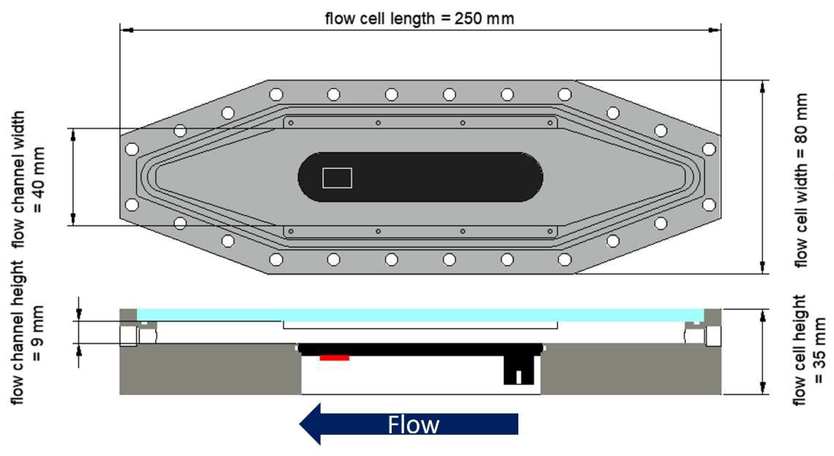
Figure 2.
Photograph of the experimental setup showing four replicates operated parallelly. Each replica was equipped with each one SST pipe, one C-PP pipe and a mesofluidic flow cell with a planar C-PP substratum. Biofilm sensors were integrated to each of the three systems. The direction of flow was from top to bottom.
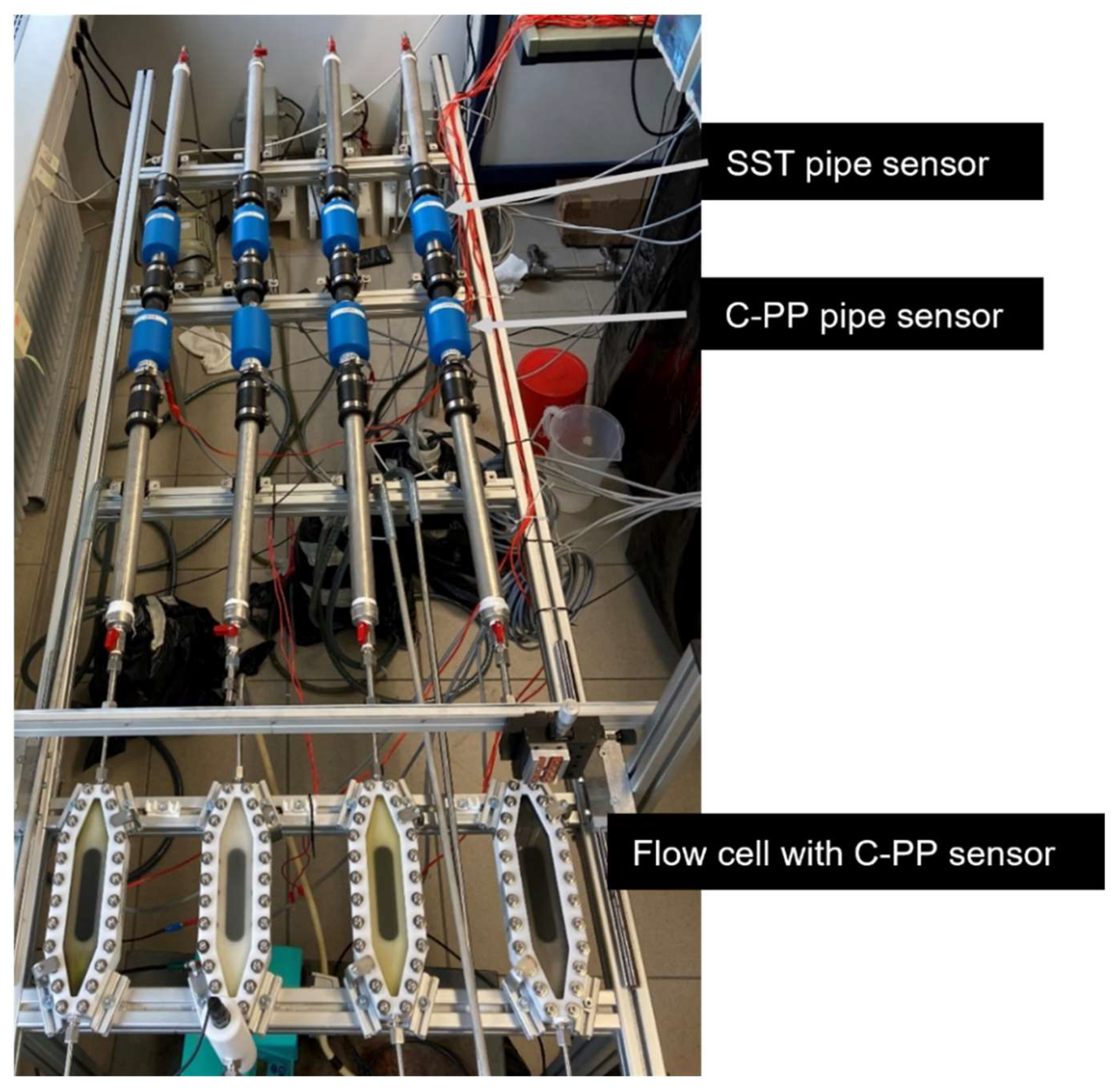
Figure 3.
(left) Development of the biofilm sensor signal over the cultivation period (t = 45 d) for the sensors integrated in the flow cells (red), SST pipes (black) and C-PP pipes (blue) at a volumetric flow rate of 2.6 L/min (Exp. 2). (right) Development of the sensor signal (top) and mean biovolume (bottom) of three replicate flow cells (A-C) in Exp. 2.
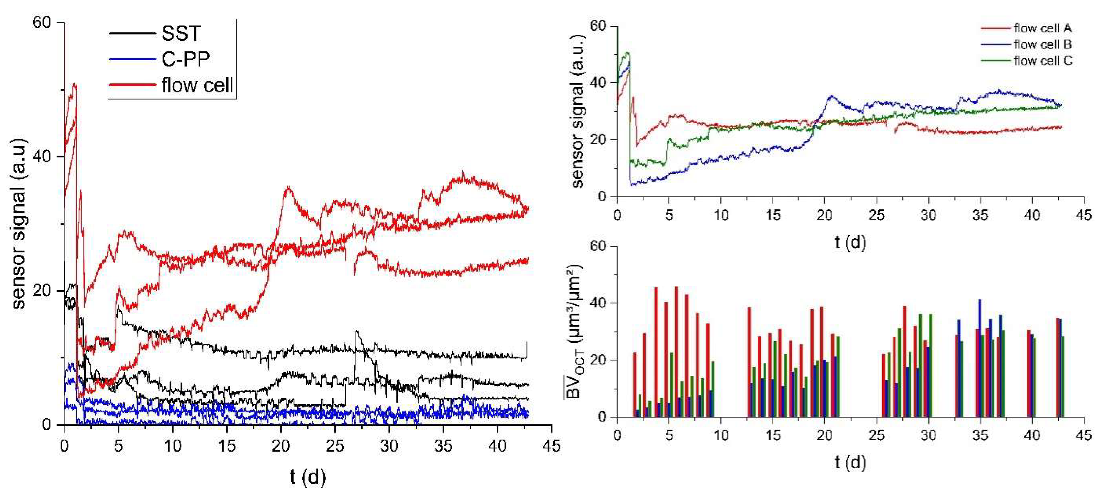
Figure 4.
Correlation of the sensor signal with the accumulated mean biovolume () at the position of the sensor on the C-PP substratum in the mesofluidic flow cells. C-scans with an imaging volume of 4 6 1 mm³ were analyzed. The acquired biovolume was correlated with the sensor signal at the time of imaging in the respective flow cell. The results of experiments 1-4 (compare Table 1) with a mean flow velocity of 9 cm/s (red), 12 cm/s (black), 16 cm/s (blue) and 27 cm/s (green) are shown.
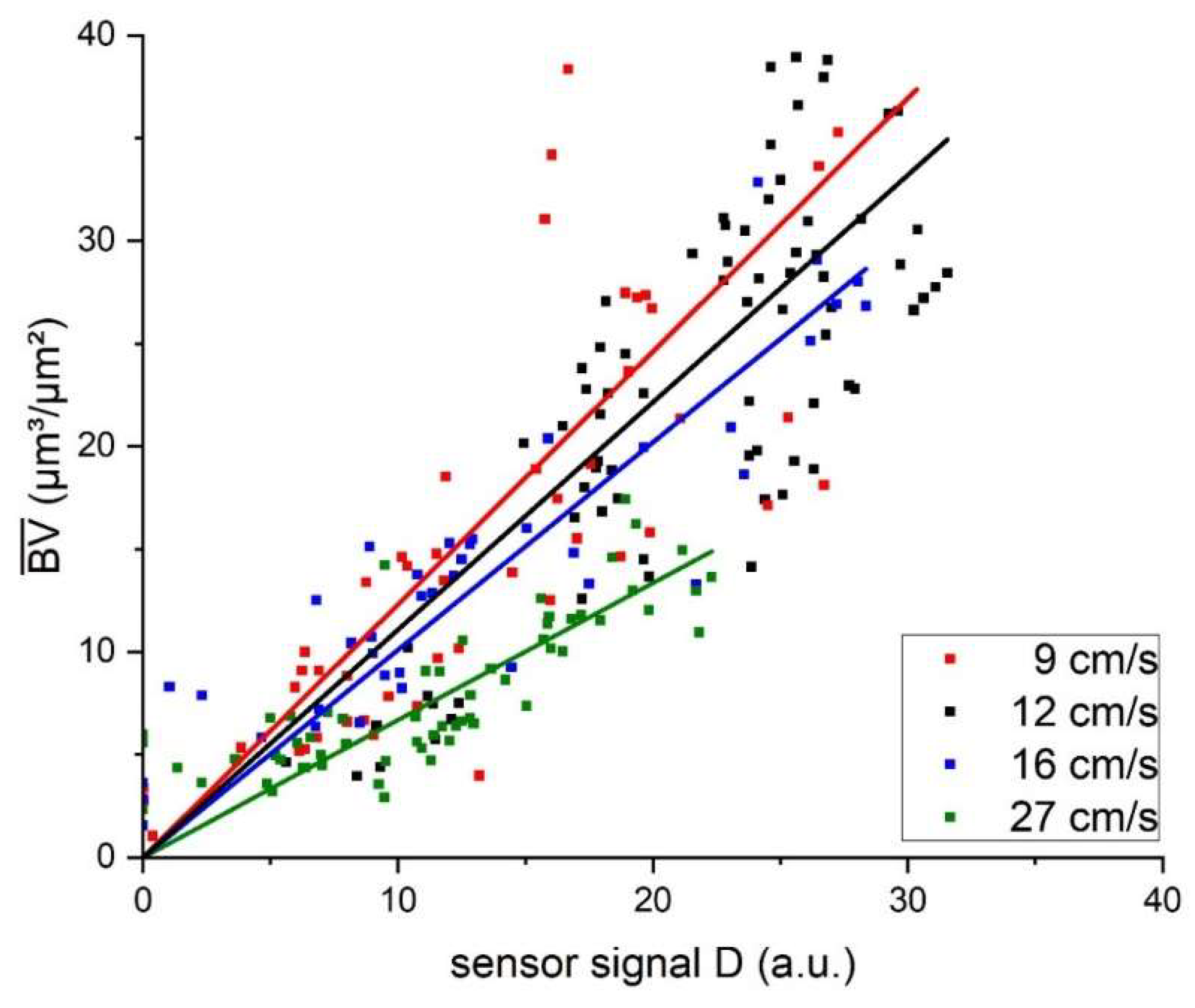
Figure 5.
Development of biofilm parameters over a period of up to 21 days for the cultivation at the linear flow velocity of 9 -27 cm/s: (A) mean biovolume, (B) mean biofilm thickness, (C) substratum coverage, (D) porosity, (E) roughness and (F) roughness coefficient. The data points displayed are the mean value of triplicates of the respective experiments. The size of the data point shows the standard deviation.
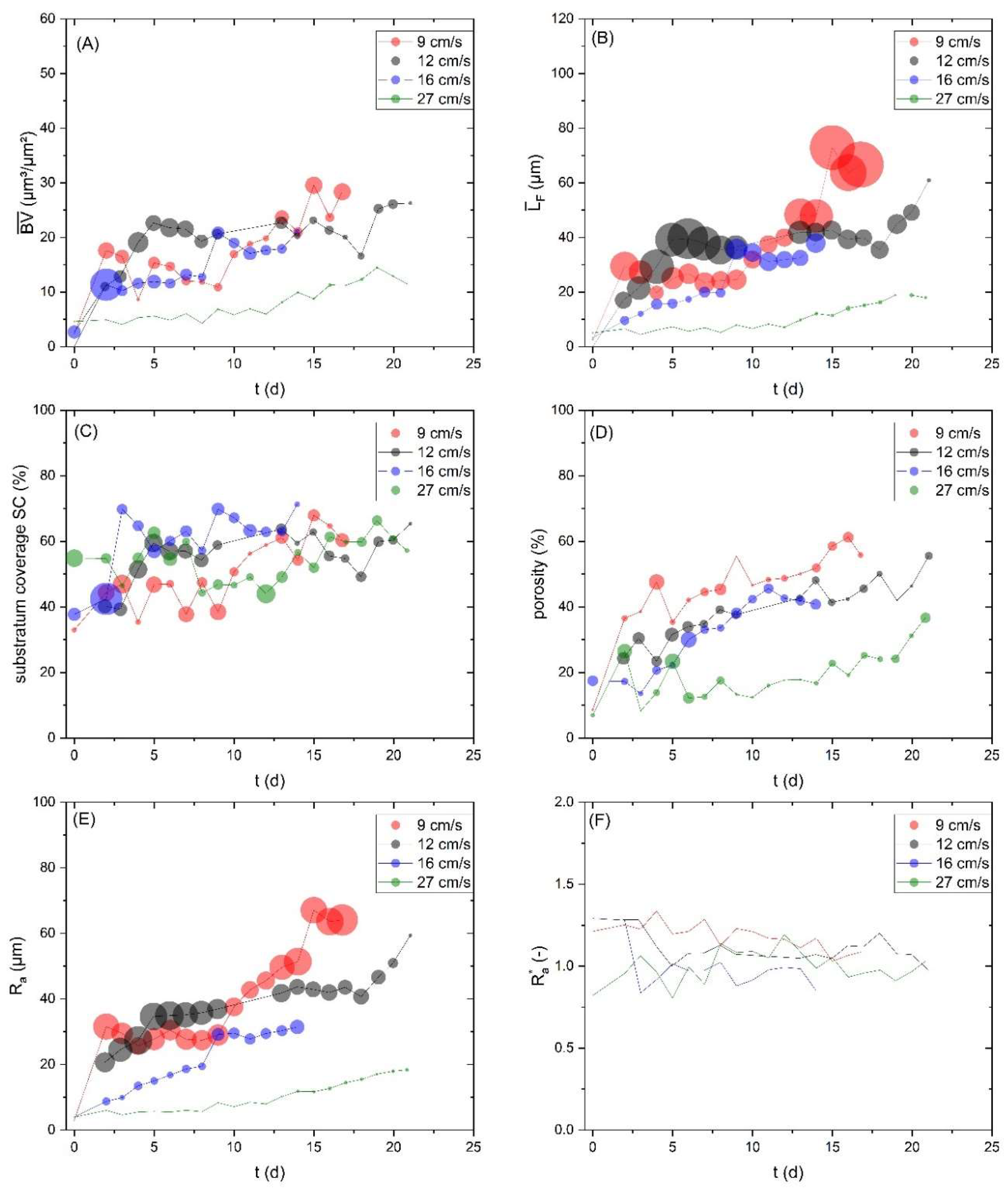
Figure 6.
(left) Calculated sensor sensitivities for the recombined flow cell combinations (triplicates) at the linear flow velocity of u = 12 cm/s. The datapoint are colored with a heatmap according to the maximum range of the mean biovolume. Warmer colored points (red) include a higher maximum mean biovolume than colder colored points (blue). The grey dashed line indicates the lower and upper limit of deviation from the mean value (p=0.05). (right) Display of all data points from the 14 investigated flow cells with the mean derived sensitivity, as well as the maximum and minimum sensitivity calculated from the triplicate recombination.
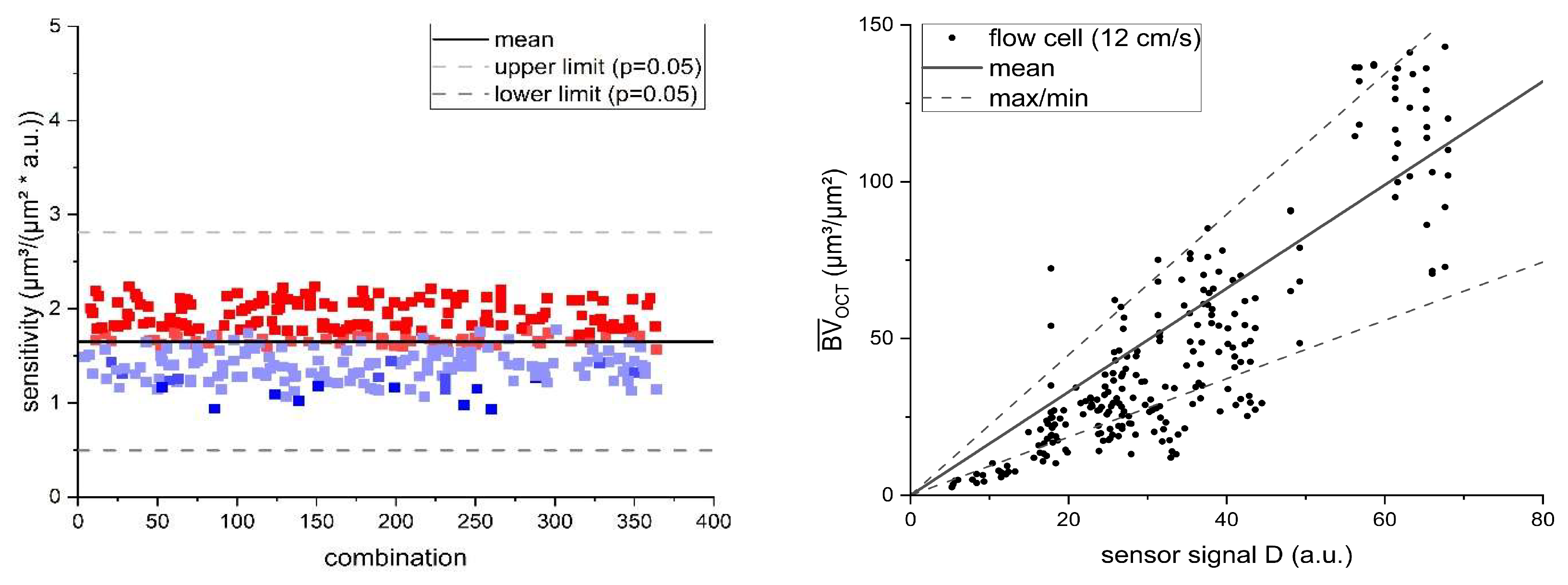
Figure 7.
Theoretical calculation of the ratio of biofilm's thermal resistance compared to the total thermal resistance of the system. The calculation was performed for the SST pipe with a linear flow velocity of 12 cm/s and the four investigated flow velocities (9-27 cm/s) in the mesofluidic flow cells with C-PP substratum. Details of the calculation are provided in the Supplementary Information (SI).
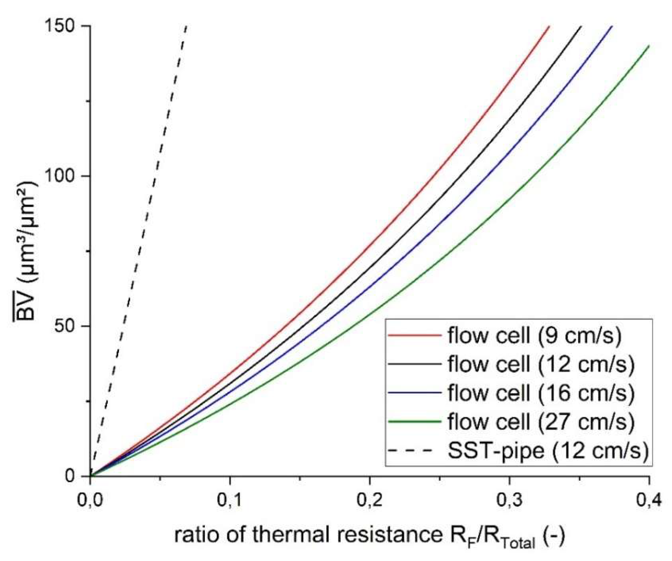
Table 1.
Overview of the experimental conditions. Each replica consisted of one SST pipe sensor, one C-PP pipe sensor and a mesofluidic flow cell with a biofilm sensor equipped to the C-PP substratum
Table 1.
Overview of the experimental conditions. Each replica consisted of one SST pipe sensor, one C-PP pipe sensor and a mesofluidic flow cell with a biofilm sensor equipped to the C-PP substratum
| Experiment | Q (L/min) | uflow cell (cm/s) | upipe (cm/s) | No. of replicates |
| 1 | 1.94 | 9 (Re = 1320) | 6.39 (Re = 1620) | 3 |
| 2 | 2.6 | 12 (Re = 1980) | 8.56 (Re = 2430) | 14 |
| 3 | 3.46 | 16 (Re = 2350) | 11.38 (Re = 2880) | 3 |
| 4 | 5.83 | 27 (Re = 3970) | 19.18 (Re = 4850) | 3 |
Table 2.
Sensitivity of the biofilm sensor calculated from the linear regression of the correlation from mean biovolume and sensor signal from experiments 1-4 (compare Table 1).
Table 2.
Sensitivity of the biofilm sensor calculated from the linear regression of the correlation from mean biovolume and sensor signal from experiments 1-4 (compare Table 1).
| Flow velocity (cm/s) | Slope of linear correlation (a.u. (µm³/µm²)) |
Sensitivity (µm³/(µm² a.u.)) | Coefficient of determination R² | Range of measured biovolume (µm³/µm²) |
| 9 | 0.81 | 1.23 | 0.89 | 0 - 38 |
| 12 | 0.92 | 1.09 | 0.94 | 0 - 39 |
| 16 | 1.02 | 0.98 | 0.95 | 0 - 33 |
| 27 | 1.49 | 0.67 | 0.93 | 0 - 18 |
Disclaimer/Publisher’s Note: The statements, opinions and data contained in all publications are solely those of the individual author(s) and contributor(s) and not of MDPI and/or the editor(s). MDPI and/or the editor(s) disclaim responsibility for any injury to people or property resulting from any ideas, methods, instructions or products referred to in the content. |
© 2025 by the authors. Licensee MDPI, Basel, Switzerland. This article is an open access article distributed under the terms and conditions of the Creative Commons Attribution (CC BY) license (https://creativecommons.org/licenses/by/4.0/).
Copyright: This open access article is published under a Creative Commons CC BY 4.0 license, which permit the free download, distribution, and reuse, provided that the author and preprint are cited in any reuse.


