Submitted:
07 January 2025
Posted:
08 January 2025
You are already at the latest version
Abstract
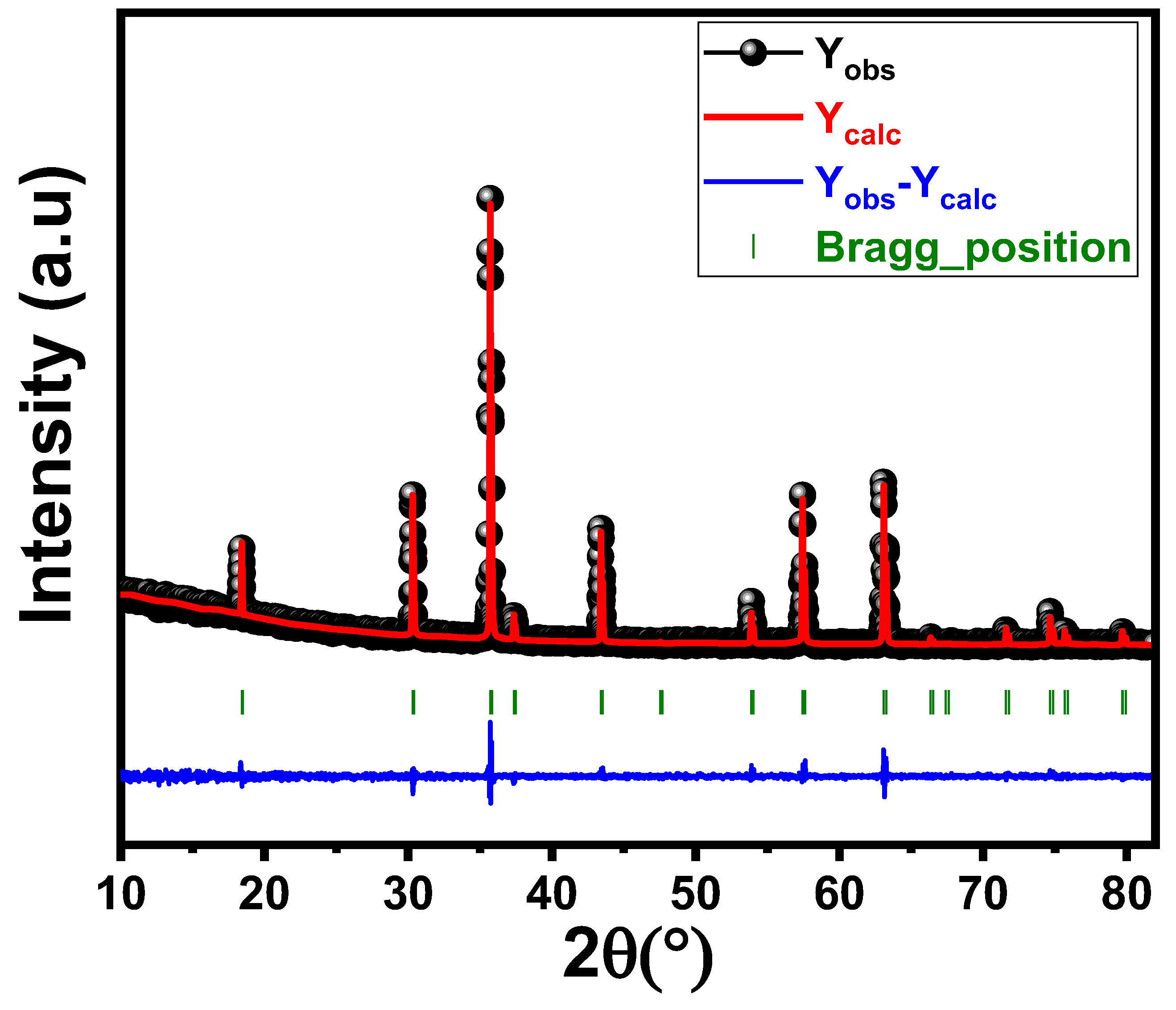
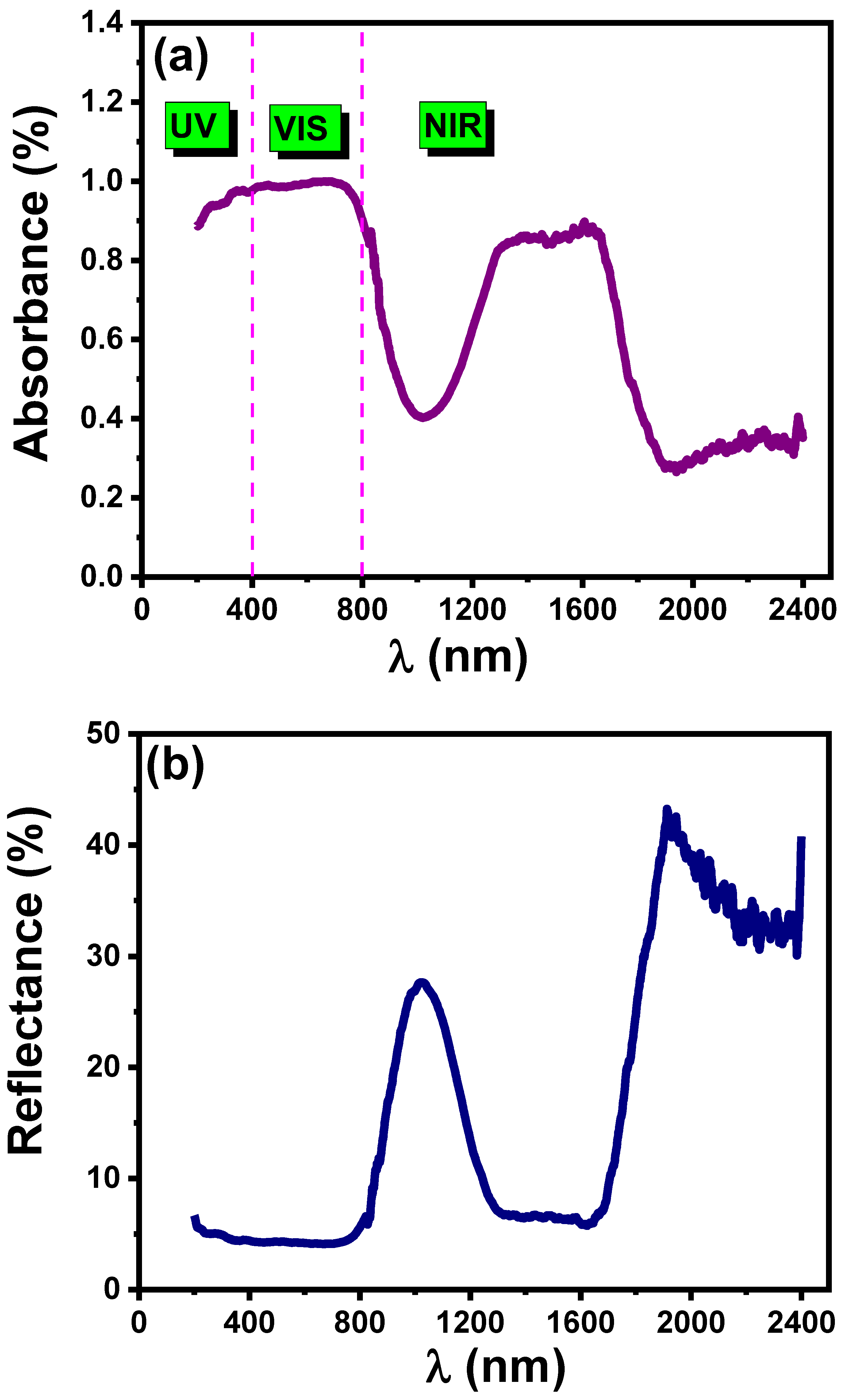
This work examines the structural, elastic, and optical properties of the Li0.5Co0.5FeCrO4 spinel ferrite. Rietveld analysis of X-ray diffraction measurement confirms its cubic spinel structure. The structural investigation reveals strong consistency among calculated and refined parameters, validating the proposed cation distribution. Elastic moduli, including bulk, longitudinal, and rigidity moduli, were acquired by computing stiffness constants. Absorbance data and the Tauc method indicated a direct optical transition with a low band-gap energy, suggesting the sample's potential for optoelectronic applications. The Li0.5Co0.5FeCrO4 spinel showed absolutely low Urbach energy, suggesting little disorder and defects within its structure. The theoretical optical characteristics like reflection loss (RL), polaron radius (Rp), molar refractive index (Rm), molar electronic polarizability (αm), and the non-linear optical features were examined for our compound. Our findings indicate that the Li0.5Co0.5FeCrO4 compound outperforms the undoped Li0.5Fe2.5O4 compound , featuring a lower band gap. This implies that adding Co and Cr into Li0.5Fe2.5O4 ferrite enhances their optical and optoelectronic applications.
Keywords:
1. Introduction
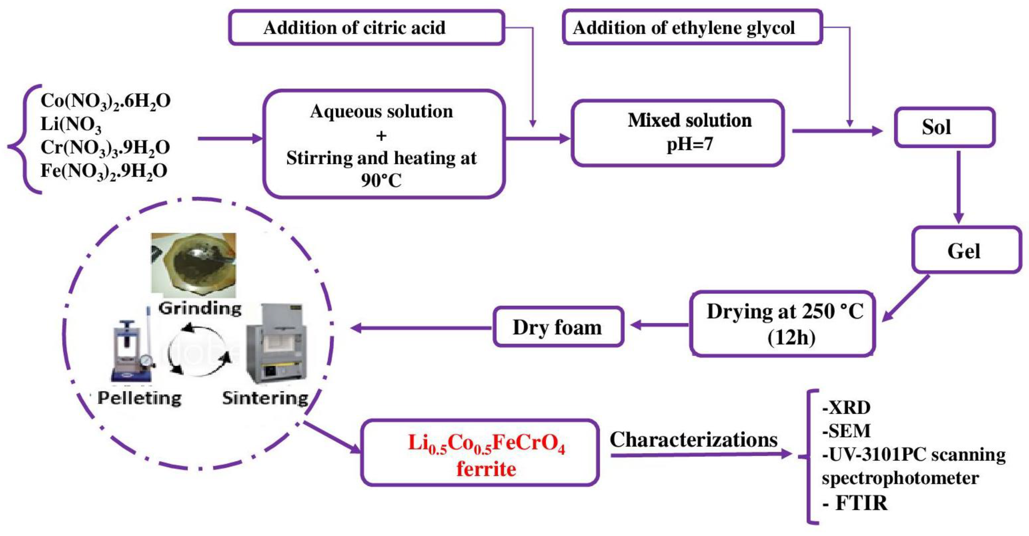
2. Experimental Details
3. Results and Discussions
3.1. Structural Properties
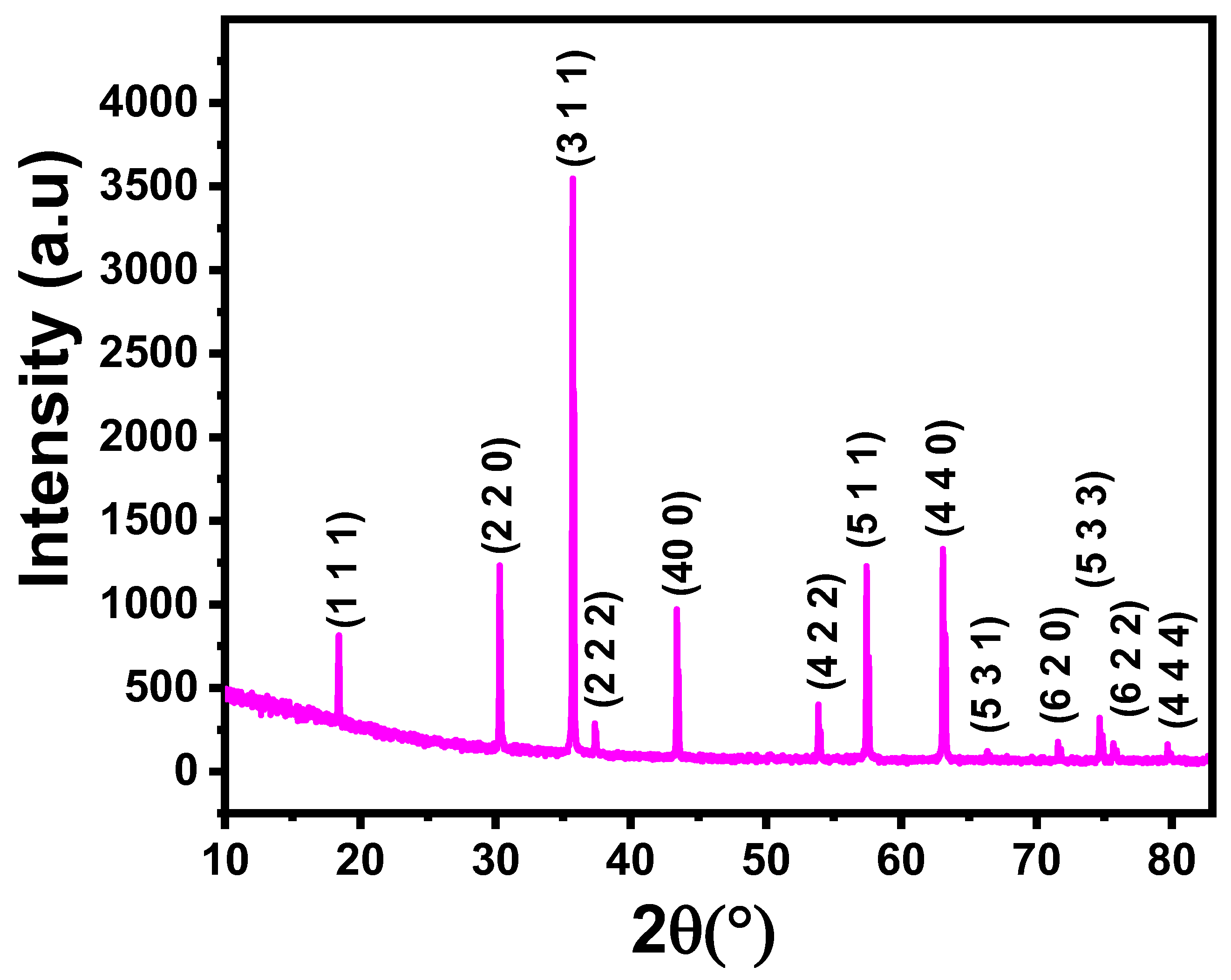
3.1.1. Rietveld Refinement
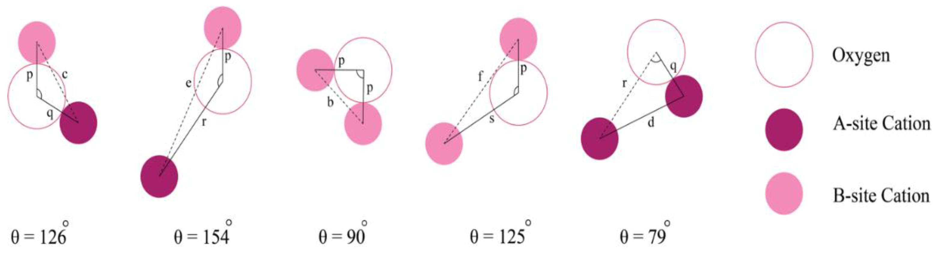
3.1.2. Theoretical Structural Parameters
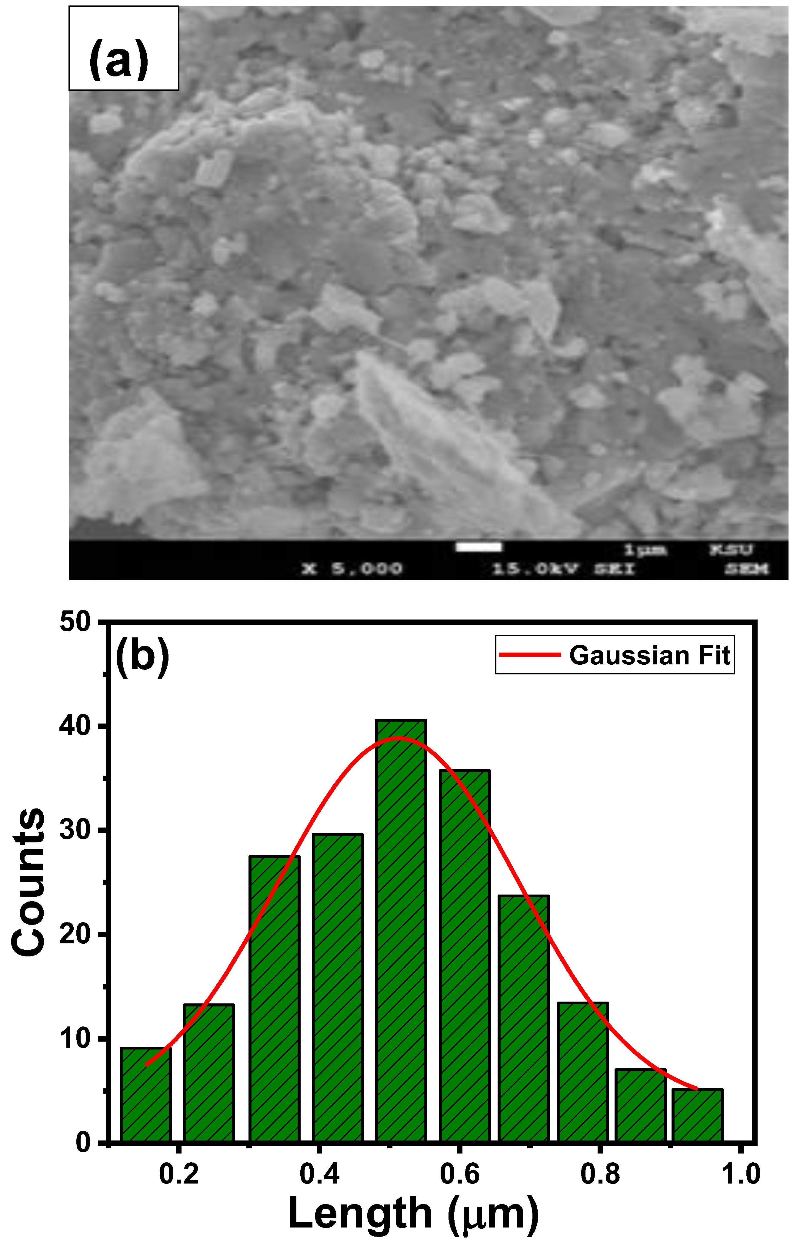
3.2. Morphological Analysis
3.3. Infrared and Elastic Properties
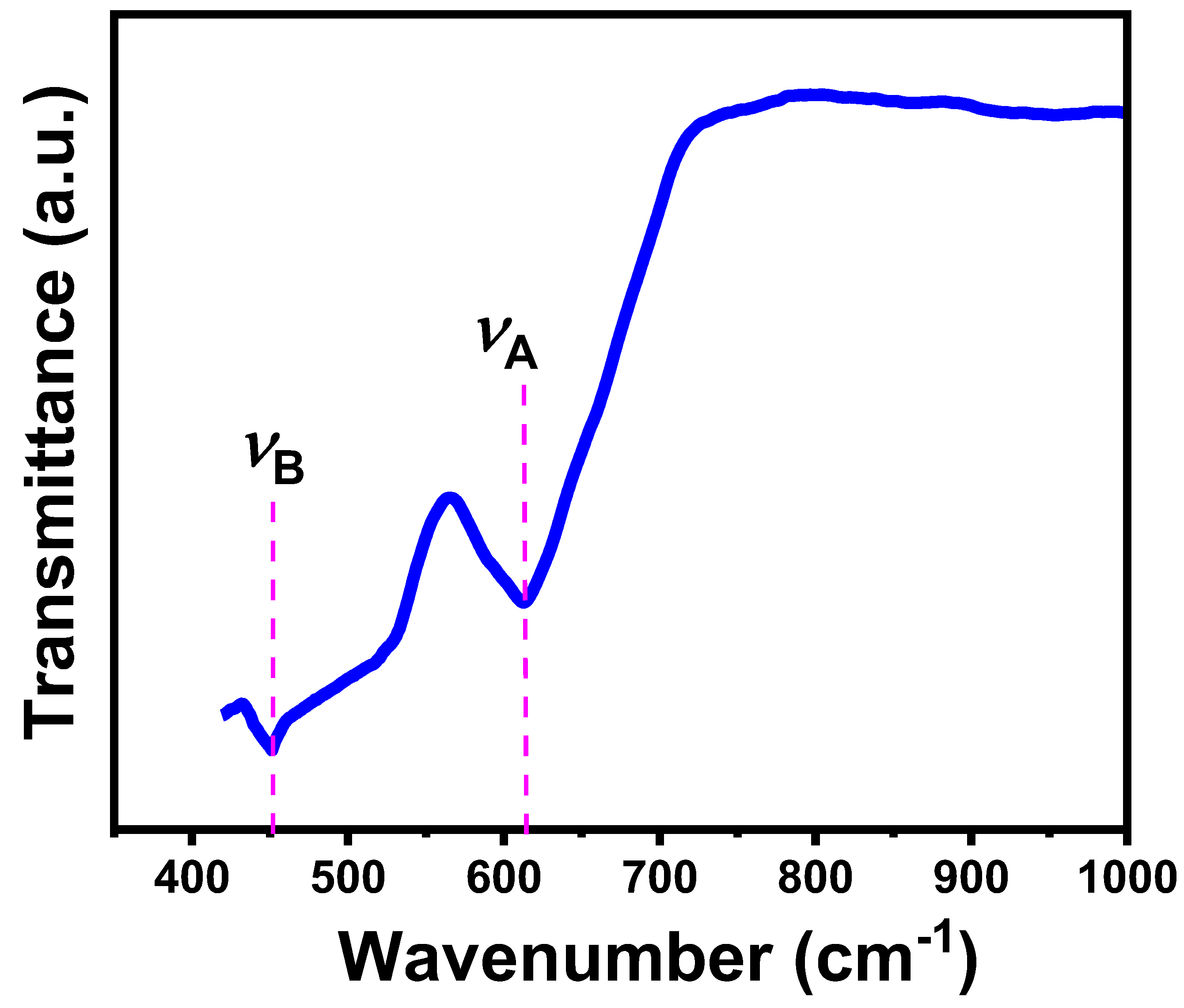
3.3.1. FTIR Spectra Analysis
3.3.2. Elastic and Thermal Properties
3.4. Optical Properties
3.4.1. UV-VIS-NIR Absorbance and Reflectance Spectra
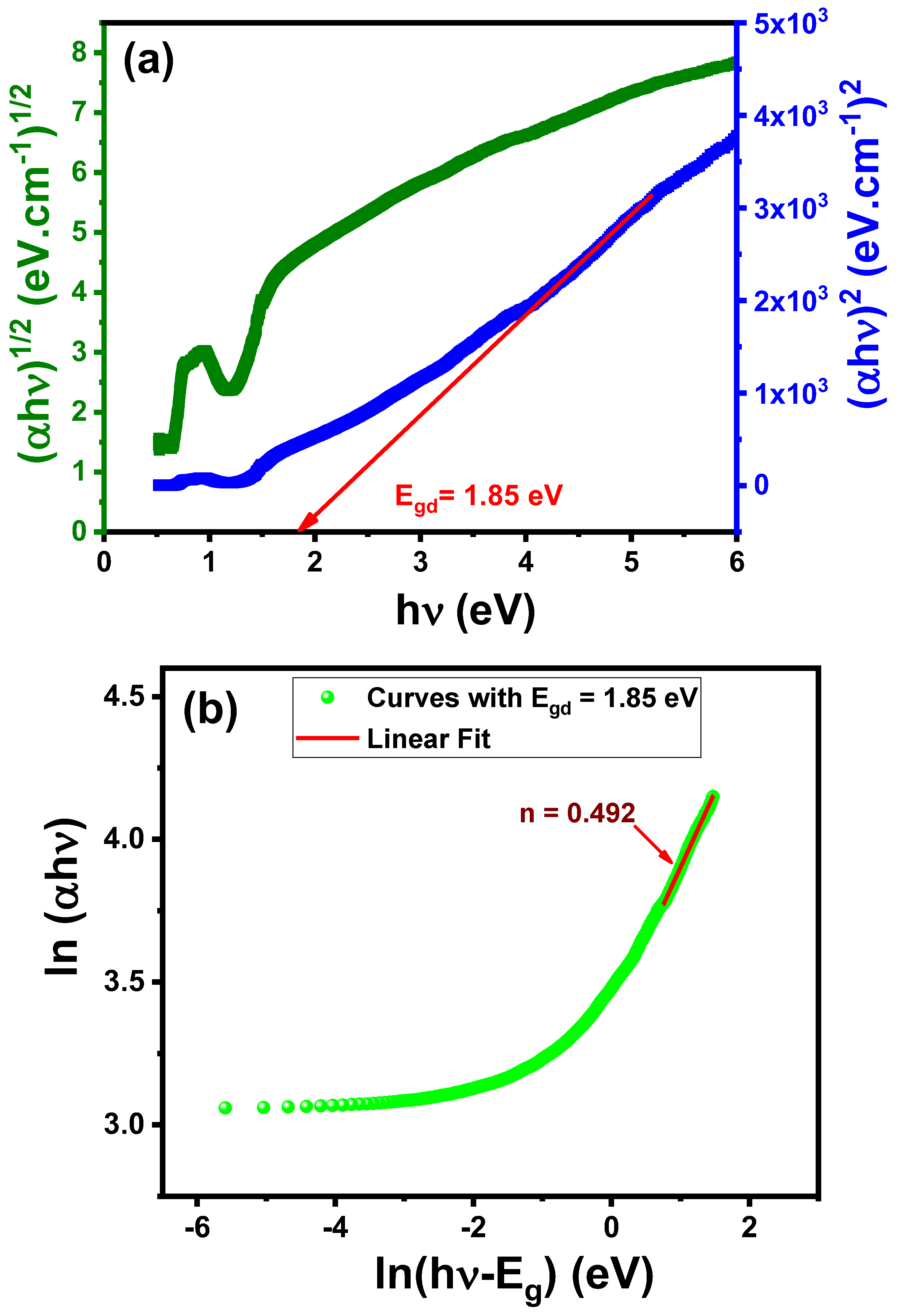
3.4.2. Optical Energy Band Gap (Eg)
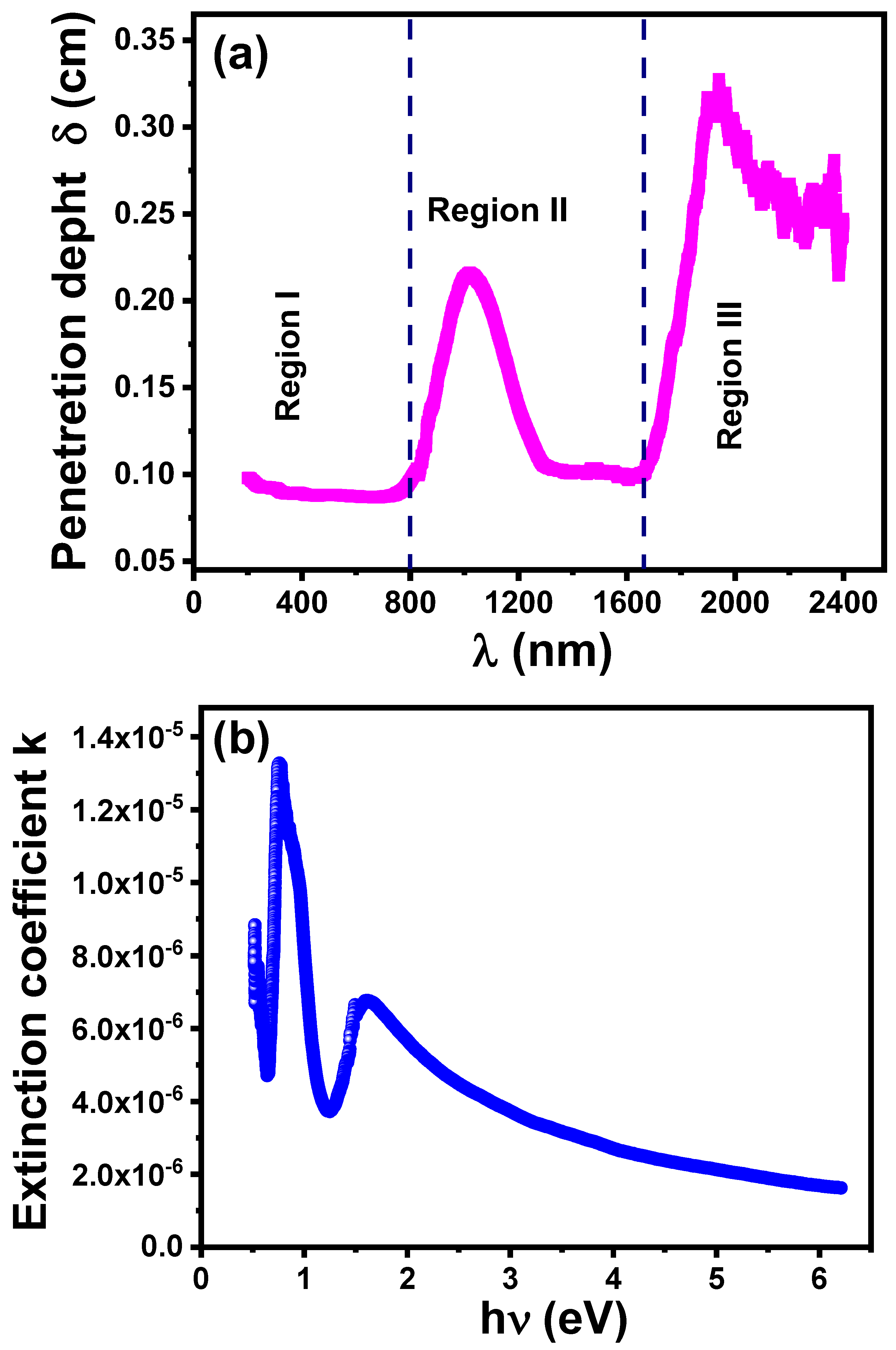
3.4.3. Penetration Depth and Extinction Coefficient
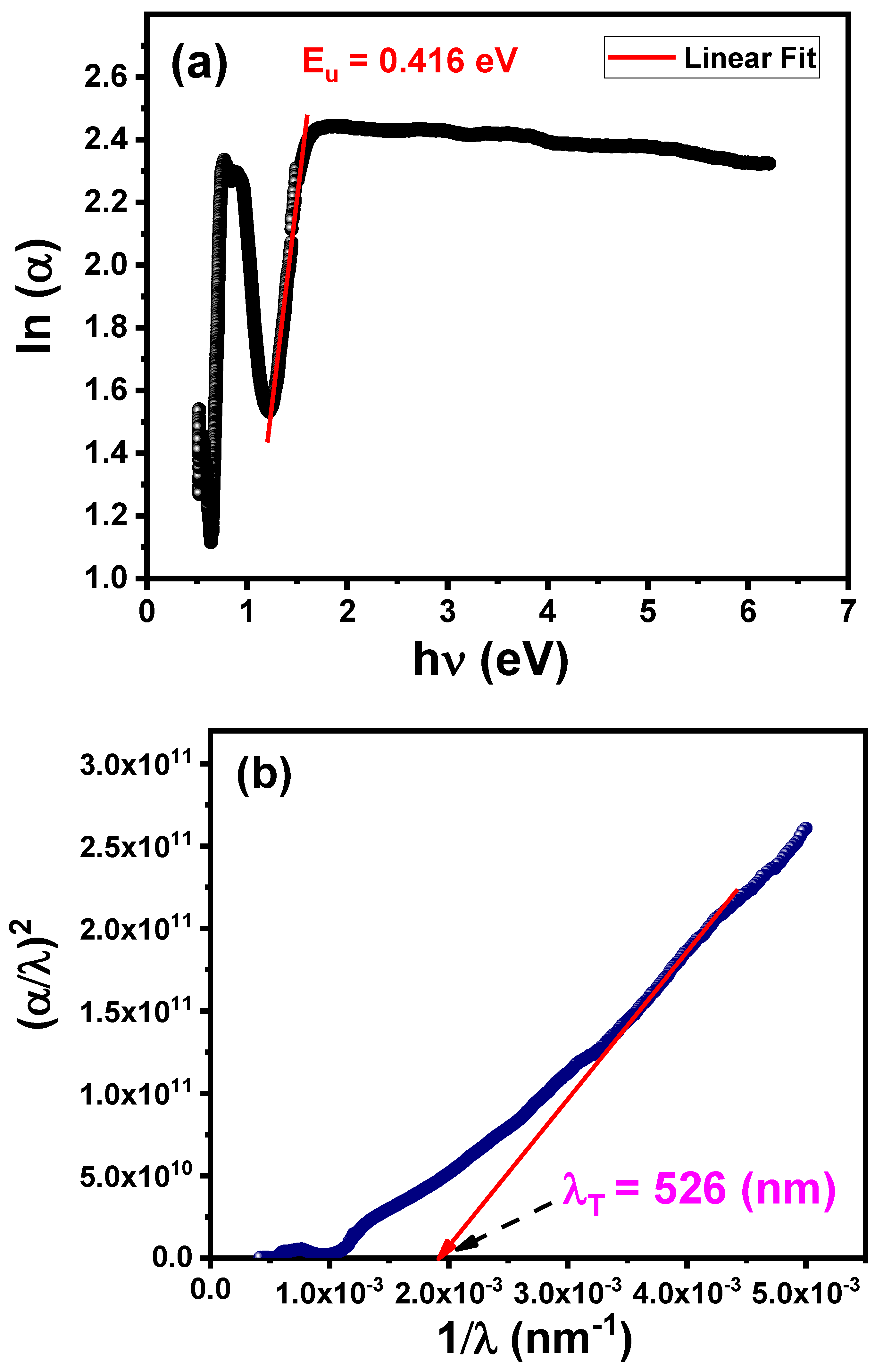
3.4.4. Urbach Energy
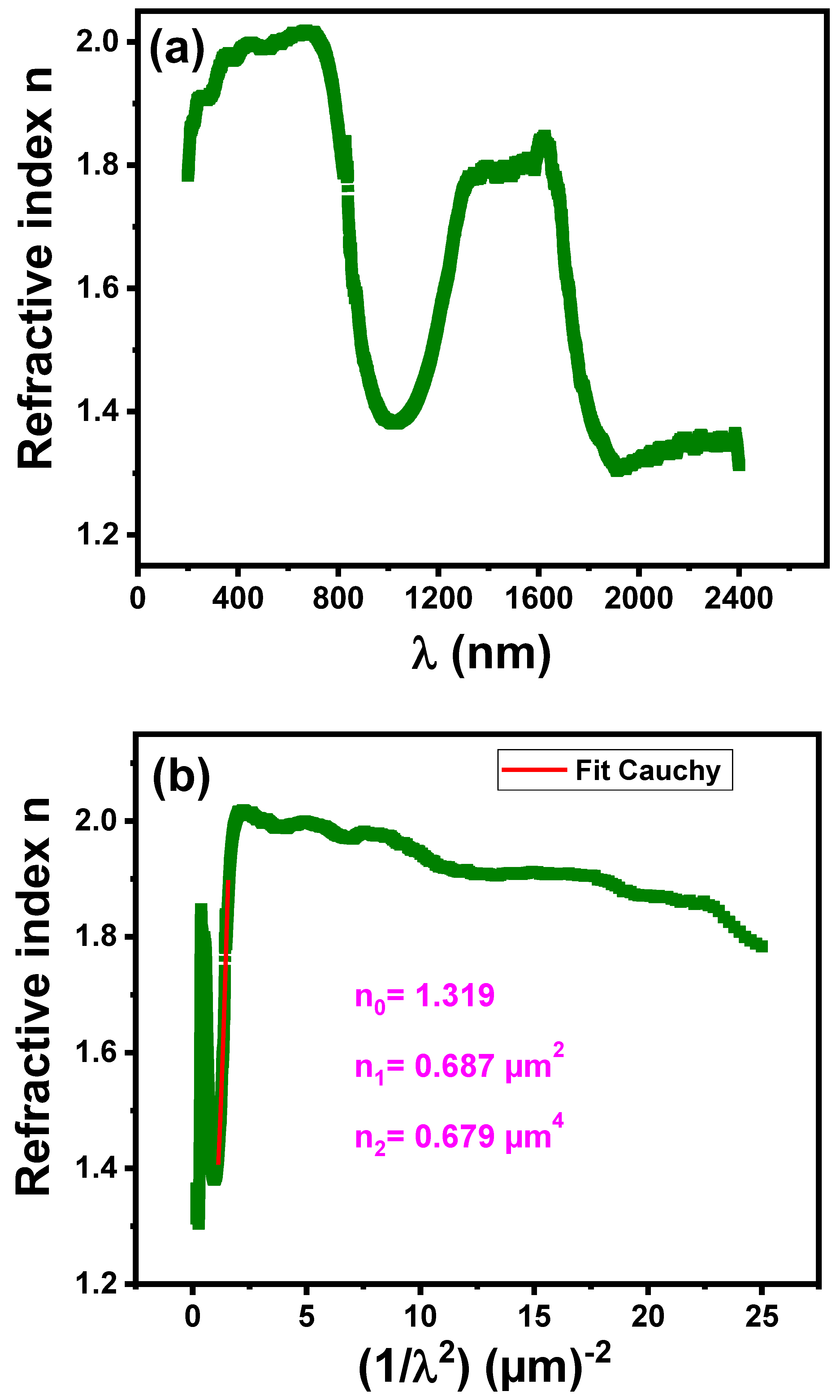
3.4.5. Refractive Index
3.4.6. Optical Conductivity and Optical Dielectric Constants
3.5. Theoretically Optical Parameters.
3.5.1. Reflection Loss (RL) and Polaron Radius (Rp).
3.5.2. Molar Refractive Index (Rm) and Molar Electronic Polarizability (αm)
3.5.3. Non-Linear Optical Parameters
4. Conclusions
References
- A.R. Sadrolhosseini, A.S.M. Noor, N. Faraji, A. Kharazmi, M.A. Mahdi, J. Nanomater. (2014) 8.
- M. S¸tefanescu, T. Dippong, M. Stoia, O. S¸tefǎnescu, J. Therm. Anal. Calorim. 94 (2008) 389.
- T. Dippong, E. Andrea Levei, O. Cadar, I. Grigore Deac, M. Lazar, G. Borodi, I. Petean, J. Alloy. Compd. 849 (2020) 156695.
- T. Dippong, E.A. Levei, C.L. Lengauer, A. Daniel, D. Toloman, O. Cadar, Mater. Charact.
- 163 (2020) 110268.
- F. Zeb, A.R. Qureshi, K. Nadeem, M. Mumtaz, H. Krenn, J. Non Cryst. Solids 435 (2016) 69.
- S. Pansambal, S. Ghotekar, S. Shewale, K. Deshmukh, N. Barde, P. Bardapurkar, J. Water Environ. Nanotechnol. 4 (2019) 186.
- C.S. Pawar, M.P. Gujar, V.L. Mathe, J. Supercond. Nov. Magn. 30 (2017) 615.
- V. Dimitrov, T. Komatsu, J. Univ. Chem. Technol. Met. 45 (2010) 219.
- M.K. Halimah, M.F. Faznny, M.N. Azlan, H.A.A. Sidek, Results Phys. 7 (2017) 589.
- K.V. Chandekar, K.M. Kant, Phys. B Condens. Matter 545 (2018) 548.
- T. Dippong, E.A. Levei, O. Cadar, Nanomaterials 11 (2021) 1560.
- N.A. Tien, V.O. Mittova, B.V. Sladkopevtsev, V.Q. Mai, I.Y. Mittova, B.X. Vuong, Solid State Sciences 138 (2023) 107149.
- M. Srivastava, S. Chaubey, A.K. Ojha, Mater. Chem. Phys. 118 (1) (2009) 174.
- M. Mayakkannan, S. Thangarasu, V. Siva, A. Murugan, A. Shameem, S. Asath Bahadur, Materials Science and Engineering: B 306 (2024) 117448.
- Atta Ur Rehman , Nasir Amin , Muhammad Bilal Tahir , Muhammad Ajaz un Nabi , N.A. Morley , Meshal Alzaid , Mongi Amami , Maria Akhtar , Muhammad Imran Arshad. Mater. Chem. Phys. 275 (2022) 125301.
- S.A.S. Ebrahimi, S.M. Masoudpanah, J. Magn. Magn. Mater. 357 (2014) 77.
- N. Kouki, S. Hcini, M. Boudard, et al., RSC Adv. 9 (2019) 1990.
- G.D. Dwivedi, K.F. Tseng, C.L. Chan, P. Shahi, J. Louremban, B. Chatterjee, A.K. Ghosh, H.D. Yang, S. Chatterjee, Phys. Rev. B 82 (2010) 134428.
- S.S. Ata-AlSmh, M.K. Fayek, H.A. Sayed, M. Yehia, Mater. Chem. Phys. 92 (2005) 278.
- A.P. Surzhikov, E.N. Lysenko, E.A. Sheveleva, A.V. Malyshev, A.L. Astafyev, V.A. Vlasov, J. Electron. Mater 47 (2018) 1200.
- Z.A. Gilani, M.S. Shifa, M.A. Khan, M.N. Anjum, M.N. Usmani, R. Ali, M.F. Warsi, Ceram. Int. 44 (2018) 1885.
- J. Huang, H. Liu, T. Hu, Y.S. Meng, J. Luo, J. Power Sources 375 (2018) 28.
- A. Mallick, A. Mahapatra, A. Mitra, J. Greneche, R. Ningthoujam, P. Chakrabarti, J. Appl. Phys 123 (2018) 055103.
- H. Zeng, T. Tao, Y. Wu, W. Qi, C. Kuang, S. Zhou, Y. Chen, RSC Advances 4 (2014) 23145.
- M. Junaid, M. A. Khan, Z. M. Hashmi, G. Nasar, N. A. Kattan and A. Laref, J. Mol. Struct., 1221 (2020) 128859.
- N. Singh, A. Agarwal and S. Sanghi, Curr. Appl. Phys. 11 (2011) 783.
- F. Gandomi, S.M.P. Motlagh, M. Rostami, A.S. Nasab, M.F. Ramandi, M.E. Arani, R. Ahmadian, N. Gholipour, M.R. Nasrabadi, M.R. Ganjali, J. Mater. Sci: Mater. Electron. 30 (2019) 19691.
- J. Jing, L. Liangchao and X. Feng, J. Rare Earths, 25 (2007) 79.
- D. Parajuli, N. Murali, V. Raghavendra, B. Suryanarayana, K.M. Batoo, K. Samatha, Appl. Phys. A 129 (2023) 502.
- P. Sharma, P. Thakur, J.L. Mattei, P. Queffelec, A. Thakur, J. Magn. Magn. Mater. 407 (2016) 17.
- A. Shokri, S. F. Shayesteh, K. Boustani, Ceram. Int 44 (2018) 22092.
- S. Singhal, S. Jauhar, J. Singh, K. Chandra, S. Bansal, J. Mol. Struct 1012 (2012) 188.
- T.R. Tatarchuk, N.D. Paliychuk, M. Bououdina, B. Al-Najar, M. Pacia, W. Macyk, A. Shyichuk, J. Alloy. Compd. 731 (2018) 1256.
- A. Iftikhar, M.U. Islam, M.S. Awan, M. Ahmad, S. Naseem, M.A. Iqbal, J. Alloy. Compd. 601 (2014) 116.
- Jitendra S. Kounsalye, Ashok V. Humbe, Apparao R. Chavan, K.M. Jadhav, Physica B: Condensed Matter 547 (2018) 64.
- P.P. Hankare, R.P. Patil, U.B. Sankpal, K.M. Garadkar, R. Sasikala, A.K. Tripathi, I.S. Mulla, J. Magn. Magn. Mater. 322 (2010) 2629.
- G. Aravind, M. Raghasudha, D. Ravinder, R.V. Kumar, J. Magn. Magn. Mater. 406 (2016) 110.
- D.R. Manea, Swati Patil, D.D. Birajdar, A.B. Kadam, Sagar E. Shirsath, R.H. Kadam, Mater. Chem. Phys.126 (2011) 760.
- M. Zulqarnain, S.S. Ali, M. Atif Yaqub, C.H. Wan, M.I. Khan, M. Riaz, A. Laref, M. Amami, Results Phys 61 (2024) 107732.
- D. Gherca, A. Pui, N. Cornei, A. Cojocariu, V. Nica, O. Caltun, J. Magn. Magn. Mater. 324 (2012) 3906.
- N. Amri, J. Massoudi, K. Nouri, M. Triki, E. Dhahri, L. Bessais, RSC Adv. 11 (2021) 13256.
- K.A. Mohammed, A.D. Al-Rawas, A.M. Gismelseed, A. Sellai, H.M. Widatallah, A. Yousif, M.E. Elzain, M. Shongwe, Physica. B. 407 (2012) 795.
- R.D. Shannon, Acta. Cryst. A. 32 (1976) 751.
- V.K. Lakhani, T.K. Pathak, N.H. Vasoya, K.B. Modi, Solid State Sci. 13 (2011) 539.
- E. Oumezzine, S. Hcini, E.K. Hlil, E. Dhahri, M. Oumezzine, J.Alloy Compd. 615 (2014) 553.
- R.D. Waldron , Physical Review. 99 (1955) 1735.
- S.C. Watawe, B.D. Sutar, B.D. Sarwade, B.K. Chougule, Int. J. Inorg. Mater. 3 (2001) 823.
- F. Hcini, S. Hcini, M. M. Almoneef, M. H. Dhaou, M. S. Alshammari, A. Mallah, S. Zemni, N. Lefi and M. L. Bouazizi, J. Mol. Struct. 1243 (2021) 130769.
- F. Hcini, S. Hcini, B. Alzahrani, S. Zemni and M.L. Bouazizi, J. Mater. Sci.: Mater. Electron. 31 (2020) 14986.
- S. Nasrin, S.M. Khan, M.A. Matin, M.N.I. Khan, A.K.M.A. Hossain, Md.D. Rahaman, J. Mater. Sci. 30 (2019) 10722.
- S.M. Patange, S.E. Shirsath, K.S. Lohar, S.G. Algude, S.R. Kamble, N. Kulkarni, D.R. Mane, K.M. Jadhav, J. Magn. Magn. Mater. 325 (2013) 107.
- K.B. Modi, J. Mater. Sci. 39 (2004) 2887.
- J. Massoudi, M. Smari, K. Nouri, E. Dhahri, K. Khirouni, S. Bertaina, L. Bessais, E.K. Hlil, RSC Adv. 10 (2020) 34556.
- A. Gholizadeh, J. Am. Ceram. Soc. 100 (2017) 3577.
- M.M. Wu, L. Wen, B. Y. Tang, L. M. Peng, W.J. Ding, J. Alloys. Compd. 506 (2010) 412.
- M.A. Islam, A.K.M.A. Hossain, M.Z. Ahsan, M.A.A. Bally, M.S. Ullah, S.M. Hoque, F.A. Khan, RSC Adv. 12 (2022) 8502.
- S.G. Algude, S.M. Patange, S.E. Shirsath, D.R. Mane, K.M. Jadhav, J. Magn. Magn. Mater. 350 (2014) 39.
- M.B. Mohamed, A.M. Wahba, Ceram. Int. 40 (2014) 11773.
- K.B. Modi, S.J. Shah, T.K. Pathak, N.H. Vasoya, V.K. Lakhani, A.K. Yahya, AIP Conf. Proc. 1591 (2014) 1115.
- Y. Gao, Z. Wang, J. Pei and H. Zhang, J. Alloys Compd. 774 (2019) 1233.
- F. Hcini, J. Khelifi, K. Khiroun, J. Inorg. Organomet. Polym 33 (2023) 3178.
- G. Raddaoui, O. Rejaiba, M. Nasri, et al., J. Mater. Sci : Mater. Electron. 33 (2022) 21890.
- O. Rejaiba, K. Khirouni, M.H. Dhaou, et al., Opt. Quantum Electron. 54 (2022) 315.
- Gagandeep, K. Singh, B.S. Lark, et al., Nucl. Sci. Eng. 134 (2000) 208.
- A. Fujishima, X. Zhang, D. A. Tryk, Surf. Sci. Rep. 63 (2008) 515.
- J. Xie, H. Wang, M. Duan, et al., Appl. Surf. Sci. 257 (2011) 6358.
- N.R. Dhineshbabu, V. Rajendran, N. Nithyavathy, et al., Appl. Nanosci. 6 (2016) 933.
- D. Erdem, N.S. Bingham, F.J. Heiligtag, N. Pilet, P. Warnicke, L.J. Heyderman, M. Niederberger, Adv. Funct. Mater. 26 (2016) 1954.
- M. L. Bouazizi, S. Hcini, K. Khirouni, M. Boudard, Optical Materials 149 (2024) 115059.
- M.A. Kassem, A.A. El-Fadl, A.M. Nashaat, H. Nakamura, J. Alloys Compd. 790 (2019) 853.
- F. Hcini, S. Hcini, M. Mohammed Alzahrani, M.L. Bouazizi, L. Haj Taieb, H. ben Bacha, Materials Today Communications 41 (2024) 111035.
- Soudani, K. Ben Brahim, A. Oueslati, A. Aydi, K. Khirouni, A. Benali, E. Dhahri, M.A. Valente, RSC Adv. 13 (2023) 9260.
- O. Amorri, H. Slimi, A. Oueslati, A. Aydi, K. Khirouni, Physica B 639 (2022) 414005.
- M. L. Bouazizi, S. Hcini, K. Khirouni, F. Najar and A. H. Alshehri, J. Inorg. Organomet. Polym 33 (2023) 2127.
- A.M. El Nahrawy, B.A. Hemdan, A.M. Mansour, A. Elzwawy, A.B. Abou Hammad, Silicon. 14 (2022) 6660.
- A.B.J. Kharrat, K. Kahouli, S. Chaabouni, Bull. Mater. Sci. 43 (2020) 275.
- B.A. Hemdan, A.M. El Nahrawy, A.F.M. Mansour, A.B. Abou Hammad, Environ. Sci. Pollut. Res. 26 (2019) 9508.
- F. Hcini, S. Hcini, M.A. Wederni, B. Alzahrani, H. Al Robei, K. Khirouni, S. Zemni, M.L. Bouazizi, Physica B 624 (2022) 413439.
- N.F. Mott, E.A. Davis, Electronic Processes in Non-crystalline Materials, Oxford university press, 2012.
- S.A. Moyez, S. Roy, J. Nanoparticle Res. 20 (2017) 5.
- A.M. Mansour, M. Nasr, H.A. Saleh, et al., Appl. Phys. A. 125 (2019) 625.
- Dhahri, F. Hcini, S. Hcini, O. Amorri, R. Charguia, K. Khirouni, J. Sol. Gel Sci. Technol. 109 (2024) 654.
- S. Husain, A.O.A. Keelani, W. Khan. Nano-Struct. Nano-Objects. 15 (2018) 17.
- A. Ben Jazia Kharrat, K. Kahouli, S. Chaabouni, Bull. Mater. Sci. 43 (2020) 275.
- A.M. Mansour, B.A. Hemdan, A.Elzwawy, A.B. Abou Hammad, A.M. El Nahrawy, Sci. Rep. 12 (2022) 9855.
- S.H. Wemple, M. Didomenico, Phys. Rev. B. 3 (1971) 1338.
- N. Tounsi, A. Barhoumi, F.C. Akkari, M. Kanzari, H. Guermazi, S. Guermazi, Vacuum 121 (2015) 9.
- A.M. Ismail, M.I. Mohammed, E.G. El-Metwally, Indian J. Phys. 93 (2019) 175.
- M.M. Abdel-Aziz, E.G. El-Metwally, M. Fadel, H.H. Labib, M.A. Afifi, Thin Solid Films 386 (2001) 99.
- H. Yokokawa, N. Sakai, T. Kawada, M. Dokiya, Solid State Ion. 52 (1992) 43.
- R. Mguedla, A. Ben Jazia Kharrat, N. Moutia, K. Khirouni, N. Chniba-Boudjada, W. Boujelben, J. Alloys. Compd. 836 (2020) 155186.
- Z. Raddaoui, B. Smiri, A. Maaoui, J. Dhahri, R. M’ghaieth, N. Abdelmoula, K. Khirouni, RSC Adv. 8 (2018) 27870.
- Y. Feng, S. Lin, S. Huang, S. Shrestha, G. Conibeer, J. Appl. Phys. 117 (2015) 125701.
- R.D. Shannon, R.X. Fischer, Phys. Rev. B Condens. Matter Mater. Phys. 73 (2006) 235111.
- N.P. Barde, V.R. Rathod, P.S. Solanki, N.A. Shah, P.P. Bardapurkar, Appl. Surf. Sci. advences 11 (2022) 100302.
- M.R. Eraky, S.M. Attia, Phys. B Condens. Matter. 462 (2015) 103.
- S. Chowdhury, P. Mandal, S. Ghosh, Mater. Sci. Eng. B 240 (2019) 120.
- W. Widanarto, M.R. Sahar, S.K. Ghoshal, R. Arifin, M.S. Rohani, K. Hamzah, M. Jandra, Mater. Chem. Phys. 138 (2013) 178.
- A. Sharma, P. Yadav, A. Kumari, AIP Conf. Proceed. 1591 (2014) 739.
- M.E. Lines, Phys. Rev. B 41 (1990) 3383.
- V. Ganesh, L. Haritha, M. Anis, M. Shkir, I.S. Yahia, A. Singh, S. AlFaify, Solid State Sci. 86 (2018) 98.
- J.J. Wayne, Phys. Rev. B 178 (1969) 1295.
- F.Z. Rachid, L.H. Omari, H. Lassri, H. Lemziouka, S. Derkaoui, M. Haddad, T. Lamhasni, M. Sajieddine, Optical Materials 109 (2020) 110332.

| Theoretical values | Refined values | |||
| Space group | ||||
| Cell parameters | a (Å) | 8.33 | 8.341 (3) | |
| V (Å3) | 578 | 580.30 (2) | ||
| Oxygen parameter | u | 0.3919 | 0.387 | |
| Oxygen parameter deviation | δ | 0.0169 | 0.012 | |
| Atoms | Tetrahedral A site (Fe) | rtet (Å) | 0.67 | - |
| Atomic positions x= y= z | 1/8 | 1/8 | ||
| Biso (Å2) | - | 1.727 (1) | ||
| Octahedral B site(Li0.5/Co0.5/Cr1) | roct (Å) | 1.41 | - | |
| Atomic positions x= y= z | 1/2 | 1/2 | ||
| Biso (Å2) | - | 0.742 (1) | ||
| O | Atomic positions x= y= z | - | 0.2590 (5) | |
| Biso (Å2) | - | 0.814 (1) | ||
| Hopping lengths | LA (Å) | 3.61 | 3.6194 (2) | |
| LB (Å) | 2.9479 | 2.951 (2) | ||
| Bond lengths | dAL (Å) | 2.05 | 1.998 (2) | |
| dBL (Å) | 1.9534 | 1.9589 (3) | ||
| Tetrahedral edge length | dAE(O-O) (Å) | 3.3476 | 3.3503(2) | |
| Shared octahedral edge length | dBE(O-O) (Å) | 2.5482 | 2.552 (1) | |
| Unshared octahedral edge length | dBEU(O-O) (Å) | 2.9614 | 2.970 (2) | |
| Me–Me distances (Å) | bB-B | 2.9471 | 2.9497 (2) | |
| cA-B | 3.4567 | 3.4531 (2) | ||
| dA-A | 3.61 | 3.621 (1) | ||
| eA-B | 5.4156 | 5.4197 (2) | ||
| fB-B | 5.1059 | 5.1172 (3) | ||
| Me–O distances (Å) | pB-O | 1.9431 | 1.9543 (2) | |
| qA-O | 2.05 | 2.03 (2) | ||
| rA-O | 3.93 | 3.942 (2) | ||
| sB-O | 3.692 | 3.685 (4) | ||
| Bond angles (°) | θA-O-B | 119.893 | 120.05 (2) | |
| θA-O-B | 145.68 | 145.45(2) | ||
| θB-O-B | 98.7 | 98.85 (2) | ||
| θB-O-B | 125.142 | 125.95 (4) | ||
| θA-O-A | 72.882 | 72.95 (2) | ||
| Agreement factors | Rp (%) | - | 6.59 | |
| Rwp (%) | - | 8.73 | ||
| RF (%) | - | 4.98 | ||
| χ2 (%) | - | 1.14 | ||
| Sample | Li0.5Co0.5FeCrO4 | |
|---|---|---|
| Absorption bands (cm-1) | υB | 452 |
| υA | 615 | |
| Force constant (N m-1) | Kt | 161.57 |
| Ko | 158.94 | |
| Kav | 160.25 | |
| Stiffness constant (GPa) | C11 | 193.31 |
| C12 | 64.43 | |
| C44 | 81.45 | |
| Wave velocity (ms-1) | υl | 6422.27 |
| υt | 3707.903 | |
| υm | 3923.24 | |
| Longitudinal modulus (GPa) | L | 192.30 |
| Rigidity modulus (GPa) | G | 63.34 |
| Bulk modulus (GPa) | B | 107.39 |
| Poisson’s ratio | σ | 0.25 |
| Pugh ratio | B/G | 1.695 |
| Debye temperature (K) | θD | 558.54 |
| Thermal conductivity (W/m.K) | Kmin | 1.178 |
| Sample | Band gap energy (eV) | Reference |
|---|---|---|
| TiO2 | 3.20 | [65] |
| ZnO | 3.37 | [66] |
| CuO | 3.85 | [67] |
| CoFe2O4 | 2.60 | [68] |
| Cu0.4Mg0.4Co0.2FeCrO4 | 1.88 | [69] |
| CoCr2O4 | 3.07 | [70] |
| Li0.5Fe2.5O4 | 3.41 | [27] |
| LiNi0.5Fe2O4 | 3.00 | [27] |
| Li0.2Co0.3Zn0.3Fe2.2O4 | 2.51 | [71] |
| LiMn0.5Fe2O4 | 3.51 | [72] |
| LiCd0.5Fe2O4 | 2.9 | [73] |
| Li0.5Co0.5FeCrO4 | 1.85 | This work |
| Sample | Li0.5Co0.5FeCrO4 |
|---|---|
| Eg (eV) | 1.85 |
| Eu (eV) | 0.416 |
| S | 0.062 |
| Ee-ph (eV) | 10.75 |
| λT (nm) | 526 |
| n0 | 1.319 |
| n1 | 0.687 |
| n2 | 0.679 |
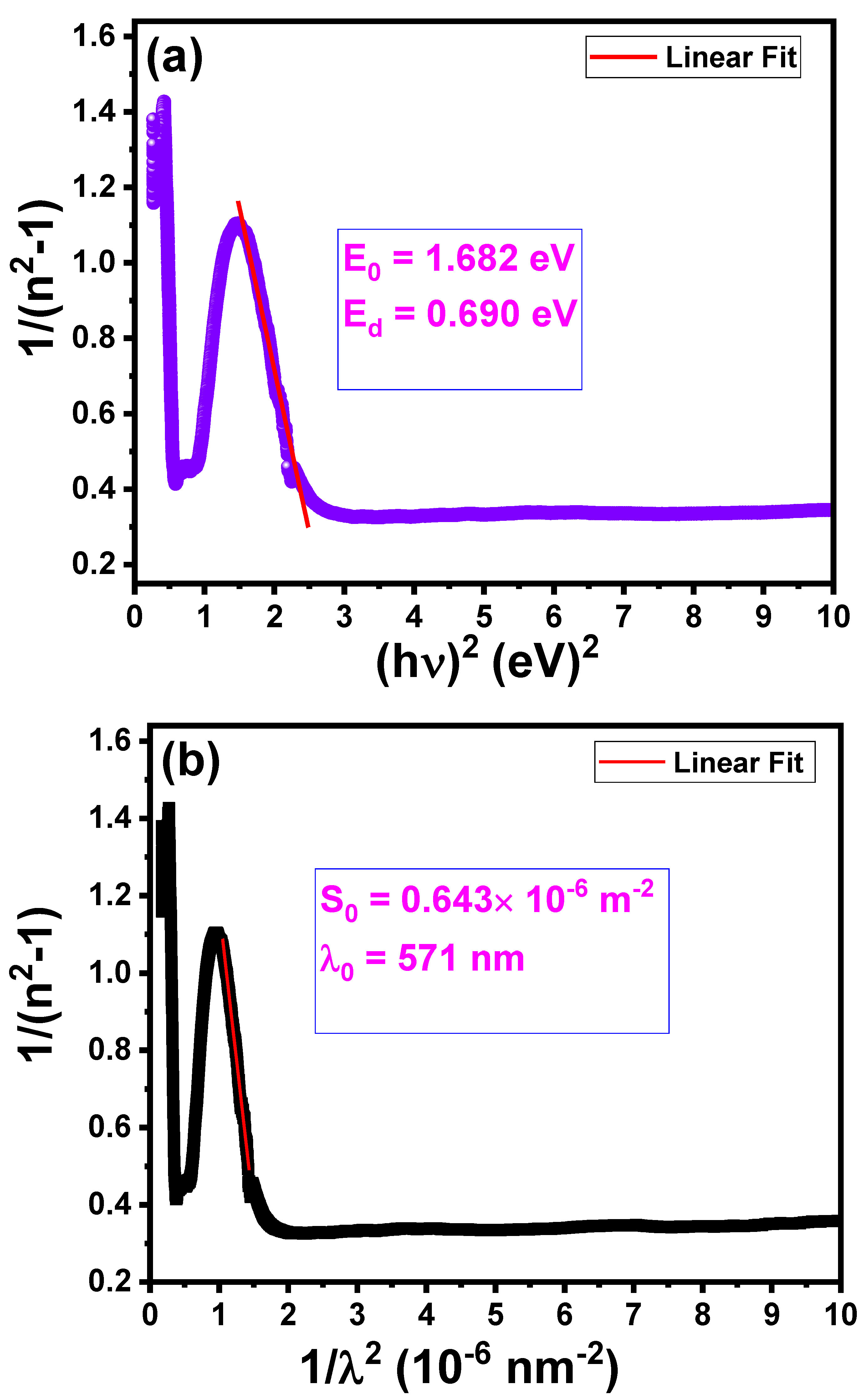
| E0 (eV) | 1.682 |
| Ed (eV) | 0.690 |
| εop | 1.41 |
| 1.187 | |
| λ0 (nm) | 571 |
| S0 (10-6 m-2) | 0.643 |
| 1.10 | |
| χ(1) (SI) | 0.032 |
| χ(3) (10-14 m2/V2) | 2.689 |
| n2 (10-13 m2/V) | 8.541 |
| Rl | 0.080 |
| Rp (Å) | 0.734 |
| αm (Å3) | 27.13 |
| Rm (Cm3/mol) | 18.75 |
Disclaimer/Publisher’s Note: The statements, opinions and data contained in all publications are solely those of the individual author(s) and contributor(s) and not of MDPI and/or the editor(s). MDPI and/or the editor(s) disclaim responsibility for any injury to people or property resulting from any ideas, methods, instructions or products referred to in the content. |
© 2025 by the authors. Licensee MDPI, Basel, Switzerland. This article is an open access article distributed under the terms and conditions of the Creative Commons Attribution (CC BY) license (http://creativecommons.org/licenses/by/4.0/).


