Preprint
Article

This version is not peer-reviewed.

Intelligent Analysis of Flow Field in Cleaning Chamber for Combine Harvester Based on YOLOv8 and Reasoning Mechanism

A peer-reviewed article of this preprint also exists.

Submitted:

04 January 2025

Posted:

07 January 2025

You are already at the latest version

Abstract

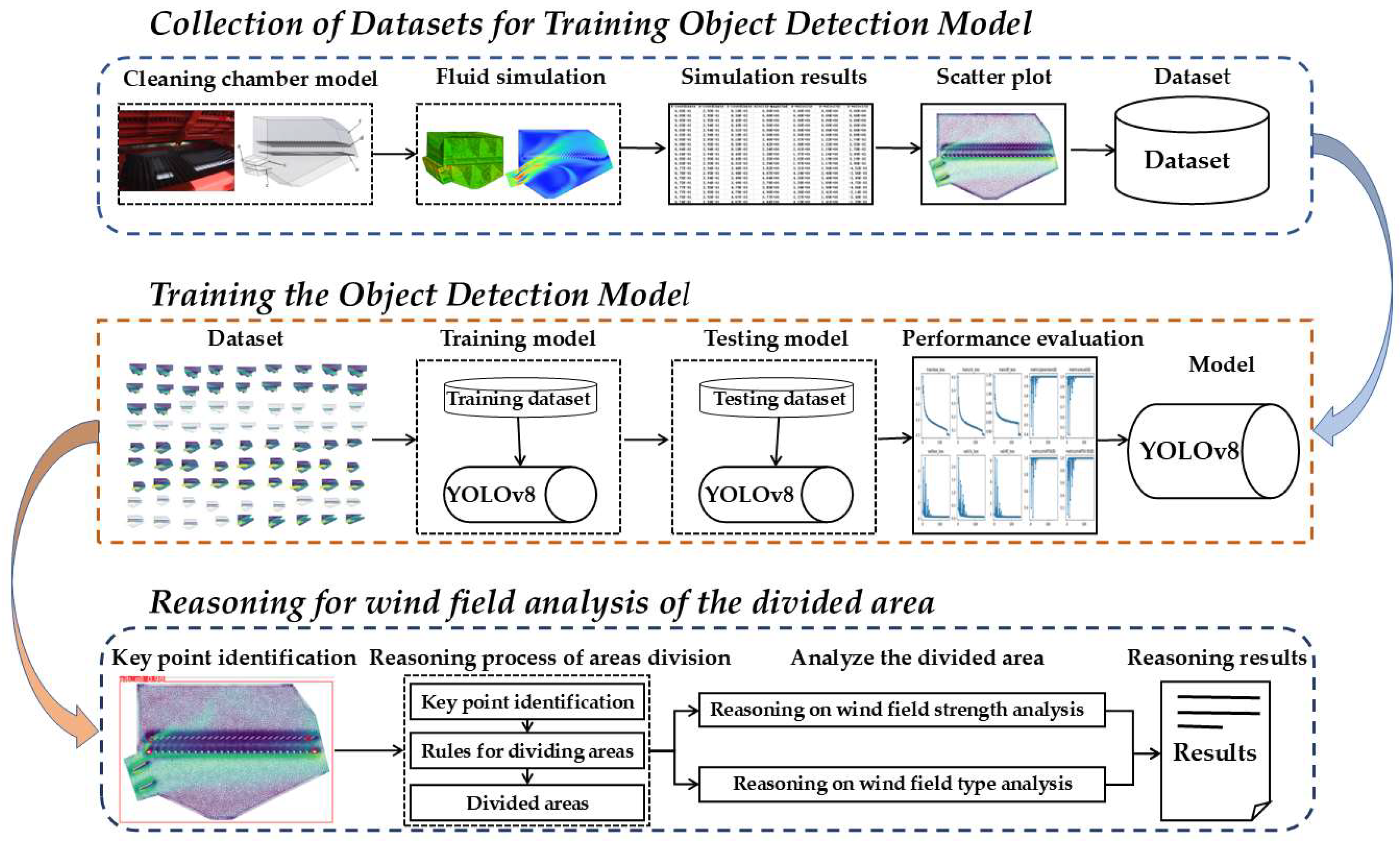
As the main working part of the combined harvester, the cleaning device affects the cleaning performance of the machine. The simulation of flow field in cleaning chamber has become an important mean of the design. Now post-processing analysis of the flow field simulation still relies on the researchers’ experience, so it is difficult to obtain information from the post-processing automatically. The experience of researchers is difficult to express and spread. This paper studied an intelligent method to analyse the simulation result data, which was based on the object detection algorithm and the reasoning mechanism. YOLOv8, one of the deep learning object detection algorithm, was selected to identify key point data from flow field in the cleaning chamber. First the training data set was constructed by scatter plot drawing, data enhancement, random screening and other technologies. Then the flow field in the cleaning chamber was divided into 6 key areas by identifying the key points of the flow field. And the analysis of the reasonable wind velocity in the areas and the cleaning results of grain were completed by reasoning mechanism based on rules and examples. Finally a system based on the above method was established by Python software. With the help of the method and the system in this paper, the flow field characteristic in the cleaning chamber and the effects of wind upon cleaning effect could be obtained automatically if the physical property of the crop, geometric parameters of the cleaning chamber, working parameters of the machine were given.

Keywords: 
;  ;  ;  ;  
Subject: 
Engineering  -   Other

1. Introduction

With the upgrading of software and hardware, the efficiency of preprocessing and solver of simulation is continuously improved. However, the post-processing data analysis of simulation is still inseparable from the engineers’ experience. As ‘ tacit knowledge ‘ [1], this kind of experience is difficult to express and disseminate. When employees leave or change jobs, the experience to analyse post-processing data can not be retained. In the absence of such ‘ experience ‘, it will be not easy for successors to succeed. Now many researchers focus on intelligent algorithms to complete judgment or diagnosis in various fields.
In the field of simulation related to mechanical design, Mingjun C has developed an automatic post-processing system with versatility and adaptability to analyse simulation result data based on the secondary development of Visual Studio and the Python built-in ABAQUS, which greatly reduces the threshold for users to obtain finite element analysis reports [2]. Wenbin L built a system combined the knowledge base and simulation post-processing of threshing device in combined harvester based on SQL Server and Visual Studio software, which solved the problems of time-consuming, cumbersome operation and low efficiency of simulation post-processing [3]. Yuying S integrated MySQL database, Java language, B/S architecture and other technologies to develop a flow field simulation post-processing and cleaning device optimization platform that includes a knowledge base management system, a simulation post-processing module and a multi-objective optimization module [4]. Ante T developed a automatic simulation and analysis system for sub-frame based on UG and ANSYS software, and realized the full automation of the whole finite element analysis process from pre-processing, solution to post-processing by combining with the transformation, preservation, extraction and acquisition of geometric features of the model [5].
In recent years, with the development and improvement of artificial intelligence, there have been many breakthroughs in key point detection algorithms and reasoning mechanisms based on deep learning.
Che J solved the problem of pedestrian image offset and attitude difference by Openpose , locating 18 key points, using attitude guidance & feature alignment to re-recognizing people with different pose, retrieving the difference and dislocation of pedestrian images [6]. Mochen L established an improved YOLOv8-Pose model to detect the key points of the stem in the red ripen stage of strawberries, which could recognize the key points of the fruit stem under complex environments [7]. Zhongfeng G proposed a key point detection method for weld feature extraction and designed a network model for weld feature extraction based on CNN, the methods can improve the accuracy and adaptability of weld recognition and ensure the quality of automatic welding because of the high detection accuracy [8].
Lu G proposed a dynamic decision-making method for weapons equipment health state based on big data, in which the K-nearest neighbor algorithm was introduced to calculate the similarity for case reasoning, and the fact feature set matching was used for rule reasoning [9]. Yu Z studied the dual reasoning mechanism of rule &case and established an expert system to diagnose the fault of the belt conveyor drive system, the accuracy rate was higher than that of the diagnostic system supported by a single reasoning mechanism algorithm [10]. Cong L screened out the automobile radiators related to the design requirements from case database by using the fuzzy evaluation algorithm, and then modified the most similar cases according to the case reasoning technology to make the cases meet the final design requirements [11]. Mengqi C studied the classification of case attributes, proposed a tree-based semantic similarity measurement method and established an expert system for aero-engine fault diagnosis based on case reasoning [12]. Lao provided an intelligent food quality assurance system composed of a case-based reasoning (CBR) engine and a fuzzy rule-based reasoning (FBR) engine, some quality assurance operations was obtained from the CBR engine, the best storage conditions for the inventory was given by the FBR engine [13]. Yi C developed a decision system to provide accurate irrigation strategies that maximize cotton yield, based on integrating the cotton model, CSM-CROPGRO, from the DSSAT model with reinforcement learning algorithms [14].
Now post-processing analysis of the flow field simulation still relies on the researchers’ experience, so it is difficult to obtain information from the post-processing automatically. In this paper, we aimed to analyze the simulation results data automatically. The simulation result data of the cleaning chamber flow field was transformed into image data,the key points was defined and identified, the regions was divided and finally the characteristics of air flow in the cleaning chamber was analysed based on the object detection algorithm, the knowledge base and the reasoning mechanism.

2. Materials and Methods

2.1. Technical Route

Firstly, the simulation result data obtained from the fluid simulation software was processed into scatter plots of key sections by visualization tools. Then scatter plots were used as the dataset for training and testing the object detection model. Finally the reasonable wind velocity in the cleaning chamber and the cleaning results of grain were analyzed based on rule reasoning (Figure 1) .

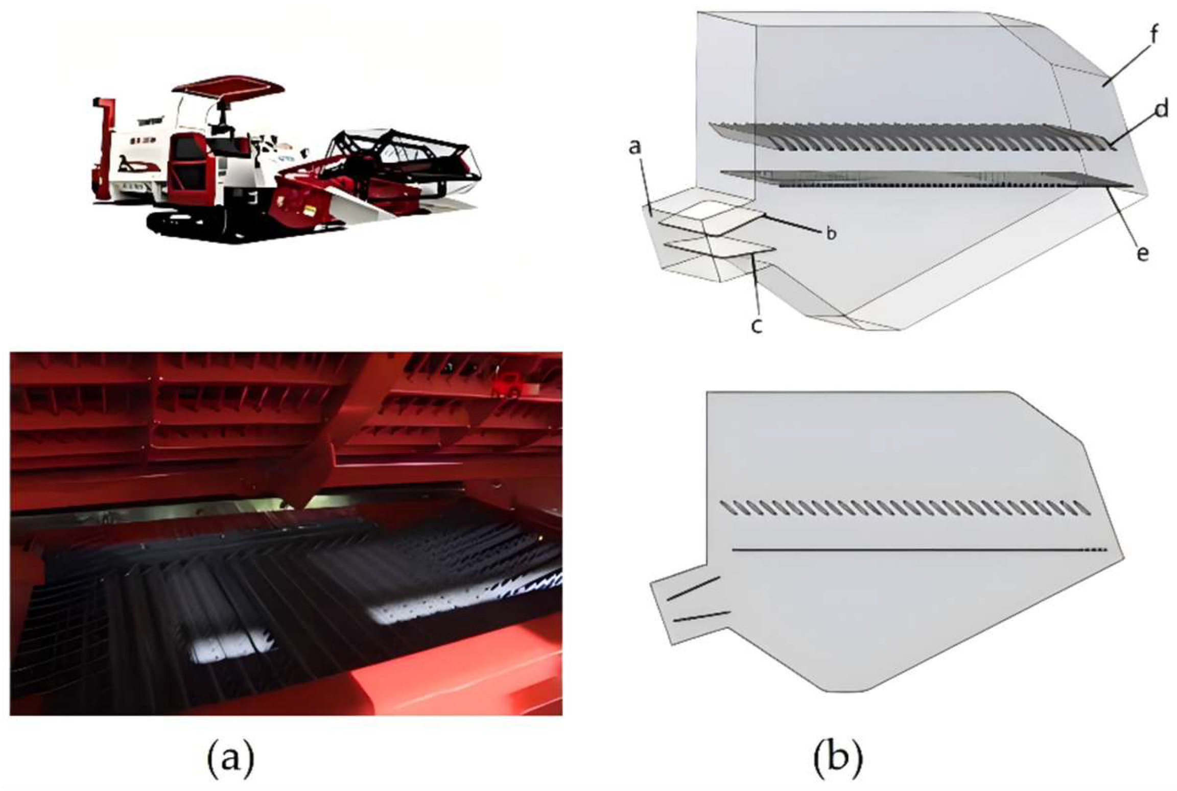
2.2. Cleaning Chamber Model

The cleaning device assembled by multiple parts with complex structure is the main working part of the combine harvester. The Lovol Gushen 4LZ-5G rice harvester is shown in Figure 2(a), the cleaning chamber was 1.0180m long and 0.840mm wide, and the cleaning sieve was a vibrating sieve. The geometric model of the cleaning device was established by SOLIDWORKS 2021(as shown in Figure 2(b)), and the airflow guide plates and the louver sieves were appropriately thickened during modeling.
A large number of cleaning chamber simulation data from different harvester were required for model training to improve the ability of the recognition model [15]. In this paper, the cleaning chamber models of 12 commonly used models were established, and the machine models and key parameters are shown in Table 1. The parameters were adjusted according to the modular design requirements: ①Change of the mesh type from louver sieve to mesh sieve by replacing half of the model lower sieve. ②Enlarge or reduce the original model to different proportions, the length range, width range and the height range of the adjusted model was respectively 700~1500mm, 490~995mm and 500~1000mm. ③Adjust the distance between the upper and lower sieves: the upper and lower sieves were offset from the original position up and down 0~150mm. As a result, a total of 216 models were remodeled and stored in 12 groups to enhance the practicality and reliability of the identification models.

2.3. Fluid Simulation Based on ANSYS Fluent Software

Combined with the structural characteristics and working conditions of the cleaning chamber, the steps of the flow field simulation of the cleaning chambers are as follows:
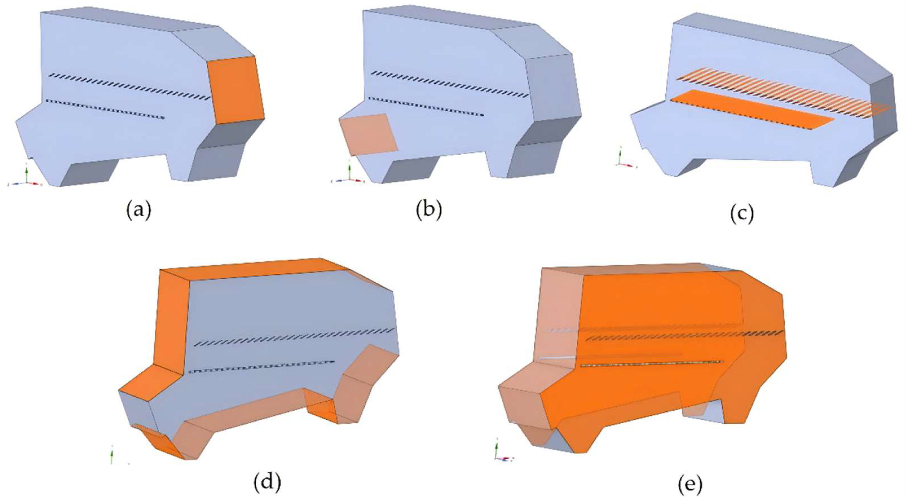
  • Pre-processing of the geometric models
The width of the model was trimmed to 1/2 by using the mirror symmetry to reduce the subsequent calculation tasks [16].
All the surfaces of the model were divided into three categories according to their functions: air outlet, air inlet and walls of the cleaning chambers. The wall surfaces of the cleaning chambers was divided into three categories according to the size of the wall: little_wall, middle_wall and big_wall, as shown in Figure 3.
2.
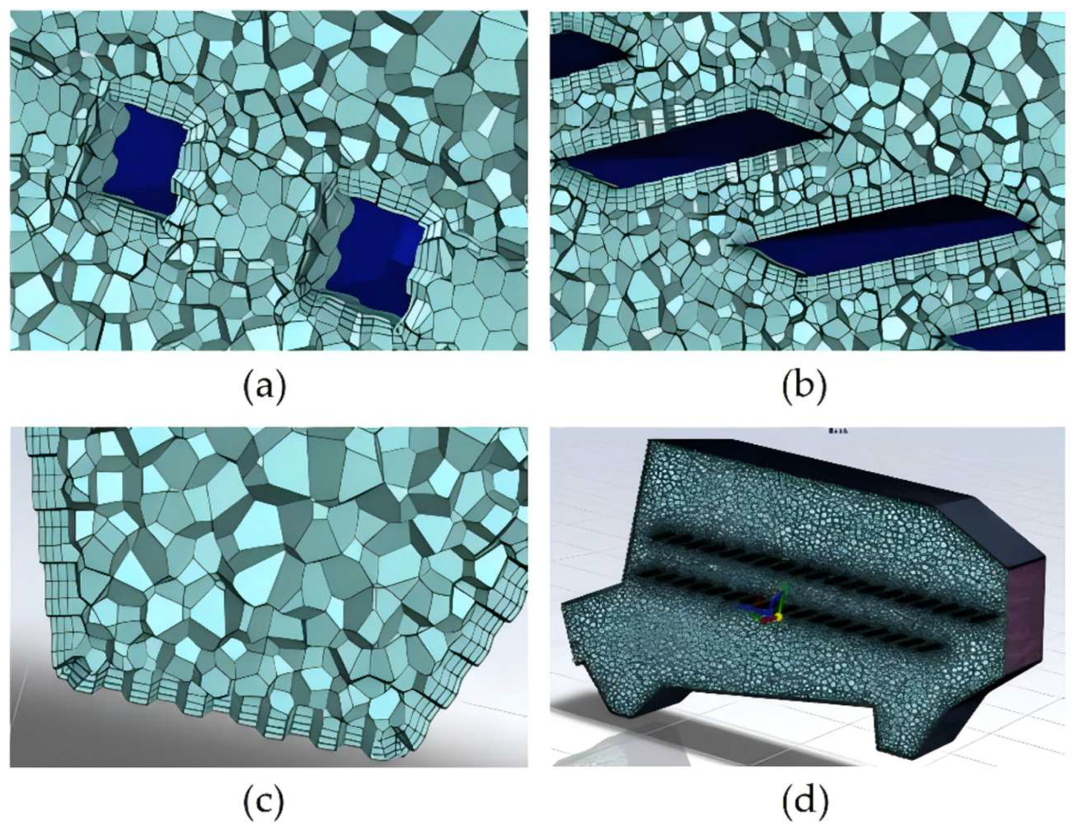
Meshing of the models
After the established geometry of the cleaning device were imported into ANSYS Fluent 2023 R1, “Watertight Geometry” was selected for workflow mode when the models were Meshing, the local dimensions were added for the surfaces, and the detailed parameters are shown in Table 2.
“Geometry type consists of only fluid areas with no voids” and “polyhedra” was selected to mesh, and the maximum element length was set to 10mm. As shown in Figure 4.
3.
Solver settings
Because the gas density in the cleaning chamber remains basically unchanged during the cleaning process, it could be regarded as an incompressible fluid, the pressure-based solver was selected [17]. The physical model was RNG k- ε turbulence model, and the wall function was standard wall function SWF. The inlet of the cleaning chamber was set to the velocity inlet, the wind velocity was set as 6~8m/s and the turbulence was set as K and Epsilon. The outlet of the cleaning chamber was set 0Pa. The solution method was SIMPLEC algorithm and the calculation would be stopped after the standard was initialized and iterated to 500 steps.

2.4. Training Model

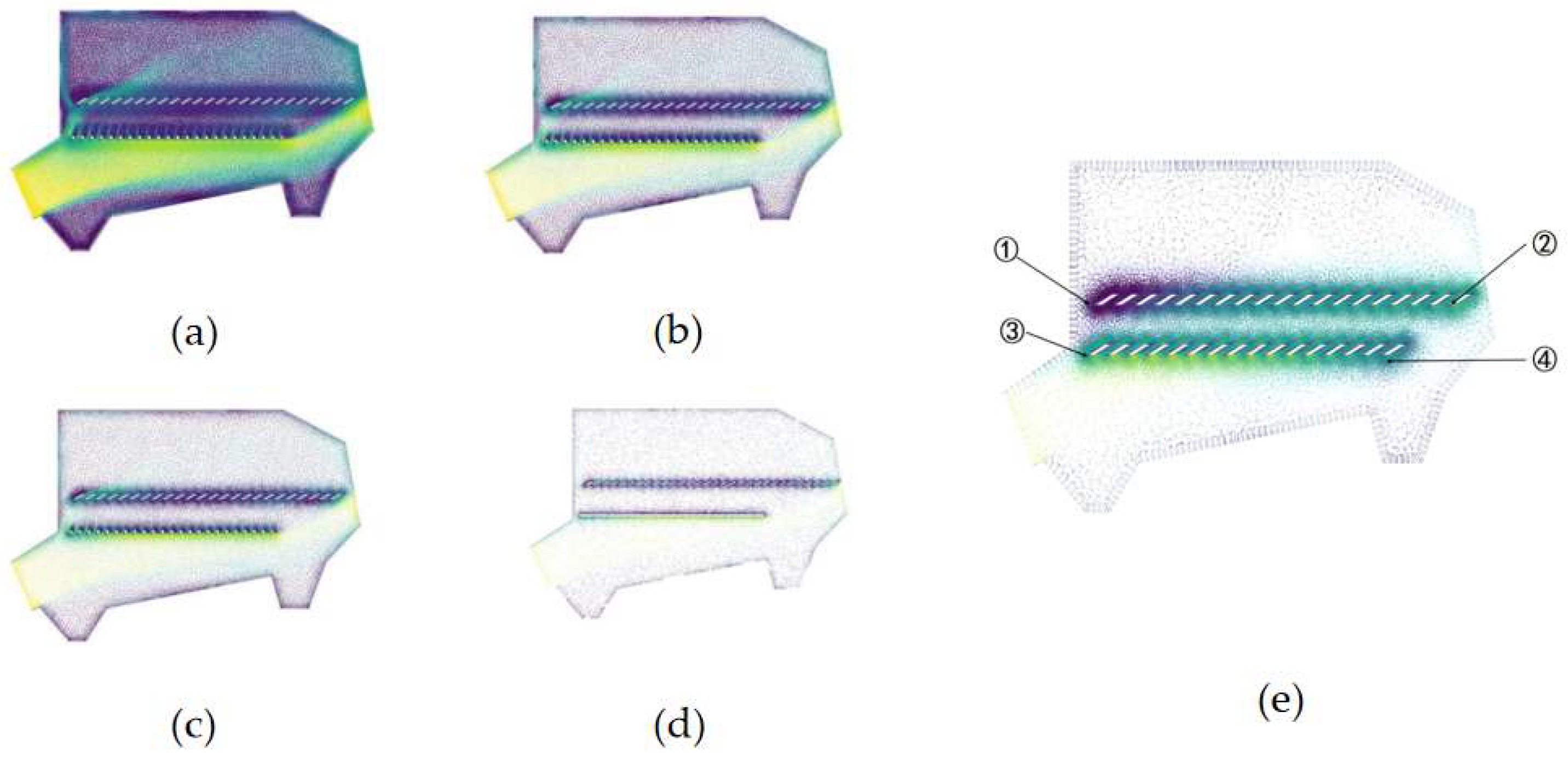
2.4.1. Construct the Dataset

The simulation results of the flow field in the cleaning chamber was the training set of the key point recognition model, which was an attempt to use the deep learning technology to the post-processing of the flow field simulation. In this paper, all the simulation results obtained in section 2.2 were studied in the form of image data.
We obtained mass data from simulation files because the size of the cleaning chamber and the number of nodes were large. Too much data would affect the processing efficiency of the algorithm. Therefore, the scattered points that could represent the characteristics of the cleaning chamber was filtered out from the massive data.
The program for screening critical cross-section data from the simulation result data was developed based on the Python and visualization tool library. The critical cross-sections that could show the position and length of the upper and lower sieves clearly were extracted(the critical cross-sections perpendicular to the Z-axis direction). The sparsity of the scatter plot was controlled by changing the thickness parameters of the critical section, Figure 5 (a) ~ (d) show the scatter plot of the key cross-section within the slice thicknesses of 2~100mm.
The mesh size near the sieve and sieve was significantly smaller than other areas [18]. Therefore, the front/rear end of the upper sieve, the front/rear end of the lower sieve could be distinguished, according to the density of the scatters. The four key points were located at the front/rear end of the upper/ lower sieve. For Kubota 4LBZ-145, the length of the cleaning chamber was 0.8755m, the height of the cleaning chamber was 0.5736m, the length of the upper &lower sieve were 0.680m and 0.700m respectively, the locations of the key points is shown in Figure 5 (e).
A total of 1188 scatter plots of cross-sections were obtained from 12 group models. As the location, orientation, and size of the scatter plots affected the reliability of the model, the data augmentation technology was used to expand the original training set [19], which included a series of transformation strategies for the image, including but not limited to random scaling, random offset, horizontal mirroring, vertical mirroring, random rotation and so on.

2.3.2. YOLOv8 Model

YOLOv8 is an advanced SOTA (state-of-ART) model developed by Ultralytics, which supports image classification, instance segmentation, object detection and tracking, etc. [20]. It builds on the YOLO series with an improved backbone which extracts image features and a detection head which predicts object locations and categories to further improve performance and flexibility.
YOLOv8 selects the decoupling head , removes the previous Objectness branch and only has the decoupled classification which is responsible for predicting the class of the object and regression branch which is responsible for predicting the location of the object. At the same time, YOLOv8 abandons the previous YOLO series of anchor bases and uses Anchor Free, which means that YOLOv8 no longer predict the object position relying on preset anchor frames, but directly predicts the center point, width and height of the target by simplifying the complexity of the model and improving the inference velocity. The improvement of the backbone is that YOLOv8 replaces the C3 module in YOLOv5 with the C2f module, which further lightens the model and obtains rich gradient flow information. In addition, YOLOv8 continues to use the SPPF module used in models such as YOLOv5, which is a spatial pyramid pooling layer and can integrate features of different scales. The main purpose is to achieve effective fusion of global features, thereby enriching the feature information of the model.
In this paper, the key points in the scatter plot of the key cross-section of the cleaning chamber needed to be identified by trying different pre-trained models. Five models were trained in the same batch, including YOLOv8n, YOLOv8s, YOLOv8m, YOLOv8l, and YOLOv8x. The scatter plots of the key cross-section obtained in 2.3.1 were used as the dataset, which was randomly divided into the training dataset and the validation dataset according to 8:2 to prevent overfitting during model training.

2.4.3. Experimental Environment and Evaluation Criteria

The experimental environment operating system in this paper was 64-bit Windows10, the memory was 64G, the graphics driver was RTX4090 and the 14-core AMDEPYC7453 processor was used. The deep learning framework of Pytorch 2.2 version was adopted, CUDAN version was 12.1 and Python version was 3.12.
The input size of the model was 640 × 640 pixels. The training batches (batch_size) was set to 16 and the initial learning rate was set to 0.01. The stochastic gradient descent method (SGD) was used to optimize the model parameters with a number of iterations of 150.
The intersection over union ( IoU ), recall ( R ), precision ( P ), average precision ( AP ) and mean average precision ( mAP )were applied to evaluate the performance of the model this paper.

2.5. Construct the Knowledge Base

The relevant knowledge of simulation post-processing of the flow field of the harvester cleaning chamber was stored in the knowledge base. The main sources of knowledge were: national standards, agricultural machinery industry specifications, factory field research, knowledge and experience of experts or engineers, professional books or design theory requirements in the field, relevant academic literature, field test data, etc. At the same time, the framework expression method or the “IF THEN” generative expression method was used to express the relevant knowledge of the post-processing of the simulation. And the knowledge of rules and examples would be stored.
The rule knowledge includes the knowledge of segmentation rules, the rules for judging the type of wind farm, the rules for comparing the actual strength and the reasonable strength of the wind farm, and the suggestions for modifying unreasonable wind conditions. The knowledge base of segmentation rules mainly stores the parameters required and knowledge which is use to segment. The knowledge base of wind field type and strength judgment rules mainly stores the parameters required for judging wind type and strength, as well as the knowledge of intensity judgment rules. The knowledge base of unreasonable wind condition modification suggestions mainly stores the types of unreasonable wind conditions, the corresponding treatment suggestions and some unreasonable wind condition modification suggestions.
The example knowledge covered the suspension velocity parameters of each component of rice & wheat. The knowledge base of the suspension velocity parameters stores the suspension velocity of each component in rice plant mixtures of varieties from different origins.The types of unreasonable wind conditions and the suggestions are mainly stored in the knowledge base of the suspension velocity parameters of each component of wheat.
All the post-processing knowledge was stored in the MySQL database in this paper, and a total of 589 post-processing related knowledge items were collected and sorted. Then, the post-processing knowledge base of simulation post-processing was established.

2.6. Post-Processing Reasoning Process of Flow Field Simulation in the Cleaning Chamber

The knowledge in the knowledge base was screened and call to give answers or feedback to the demand questions with the help of reasoning.
In the post-processing of the flow field simulation, the simulation results were different under different cleaning chamber sizes and different parameter settings, and even if a large amount of example knowledge were stored, it was still difficult to match the similarity of the examples in the face of a new cleaning chamber design [21]. Therefore, the example-based inference mechanism and the rule-based inference mechanism were selected according to the characteristics of simulation results.
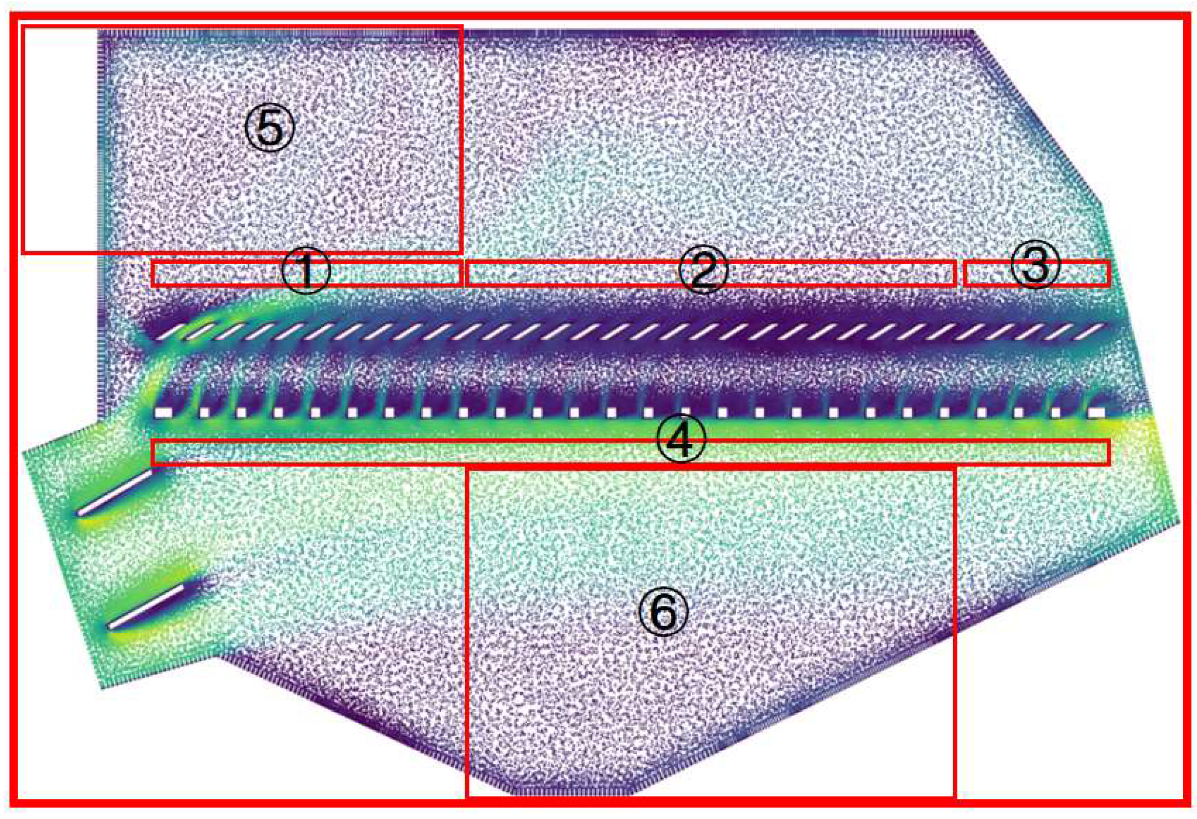
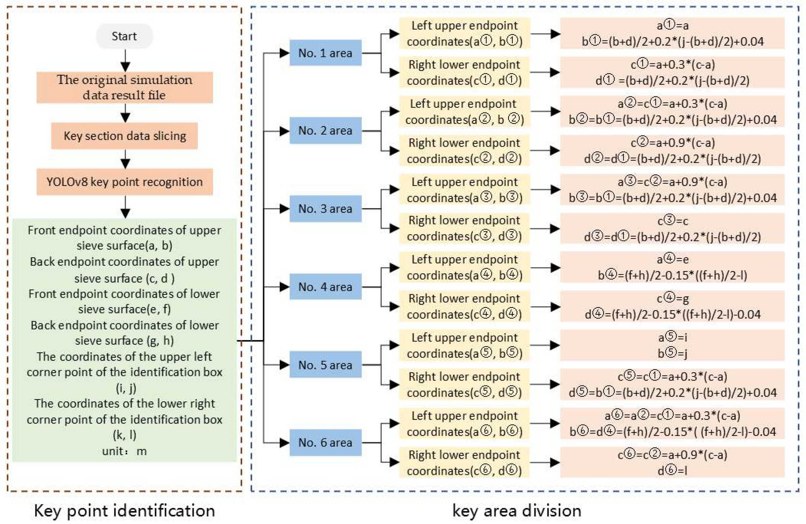
  • Reasoning process for key area division of flow field in the cleaning chamber
In the simulation post-processing stage, there are six areas where researchers pay most attention to, as shown in Figure 6.
The location judgment rules and wind field analysis method of each region are as follows:
No.1 area: It was located above the upper sieve surface of the front segment, the length was 30% of the total length of the upper sieve and the left side of the area was aligned with the left side of the upper sieve surface. The intensity of the wind field in this region determines whether the grain mixture input through the jitter plate or feeding device could enter the No.2 area smoothly, avoiding the grain mixture falling in the No.1 area and affecting the grain falling into the sieve hole, which was related to the cleaning efficiency.
No.2 area: It was located above the upper sieve surface in the middle section, the length accounts for 60% of the total length of the upper sieve and the left side of the area was adjacent to the right side of the No.1 area. The intensity of the wind field in this region determines whether the materials blown from the No.1 area could be blown away smoothly and cleans preliminarily, which affected the cleaning efficiency and the cleaning loss rate.
No.3 area: It was located above the upper sieve of the rear segment, the length accounts for 10% of the total length of the upper sieve and the right side of the area was aligned with the right side of the upper sieve. The intensity of the wind field in this region determines whether the impurities in the material mixture could be cleaned successfully and affected the impurity content of the cleaning.
No.4 area: It is located below the lower sieve surface, the length was equal to the lower sieve surface and the left side of the area was aligned with the left side of the lower sieve surface. The intensity of the wind field in this region determines whether all impurities in the material mixture, except the grains, could be effectively separated and blown out of the cleaning chamber. Suitable wind velocity could greatly reduce the impurity content of cleaning.
No.5 area: It was located directly above No.1 area, the left side was aligned with the leftmost end of the cleaning chamber and the right side was aligned with the right side of No.1 area. There was the possibility of eddy in this region. If the eddy was relatively complete and strong, the impurities in the grain mixture would be affected by the eddy and confine to a certain area, which would adversely affect the cleaning efficiency.
No.6 area: It was located below No.4 area, the left side was aligned with the left side of No. 2 area and the right side was aligned with the right side of No.2 area. There might be eddy in this region. If the eddy was relatively complete and strong, the impurities in the grain mixture would be affected by the eddy and repeatedly tumble above the grain collection site without being cleared, which would cause the impurity content of the cleaning to increase.
The division process of the six detection areas in the cleaning chamber is shown in Figure 7, combining with the detection results of YOLOv8 on key point coordinates.
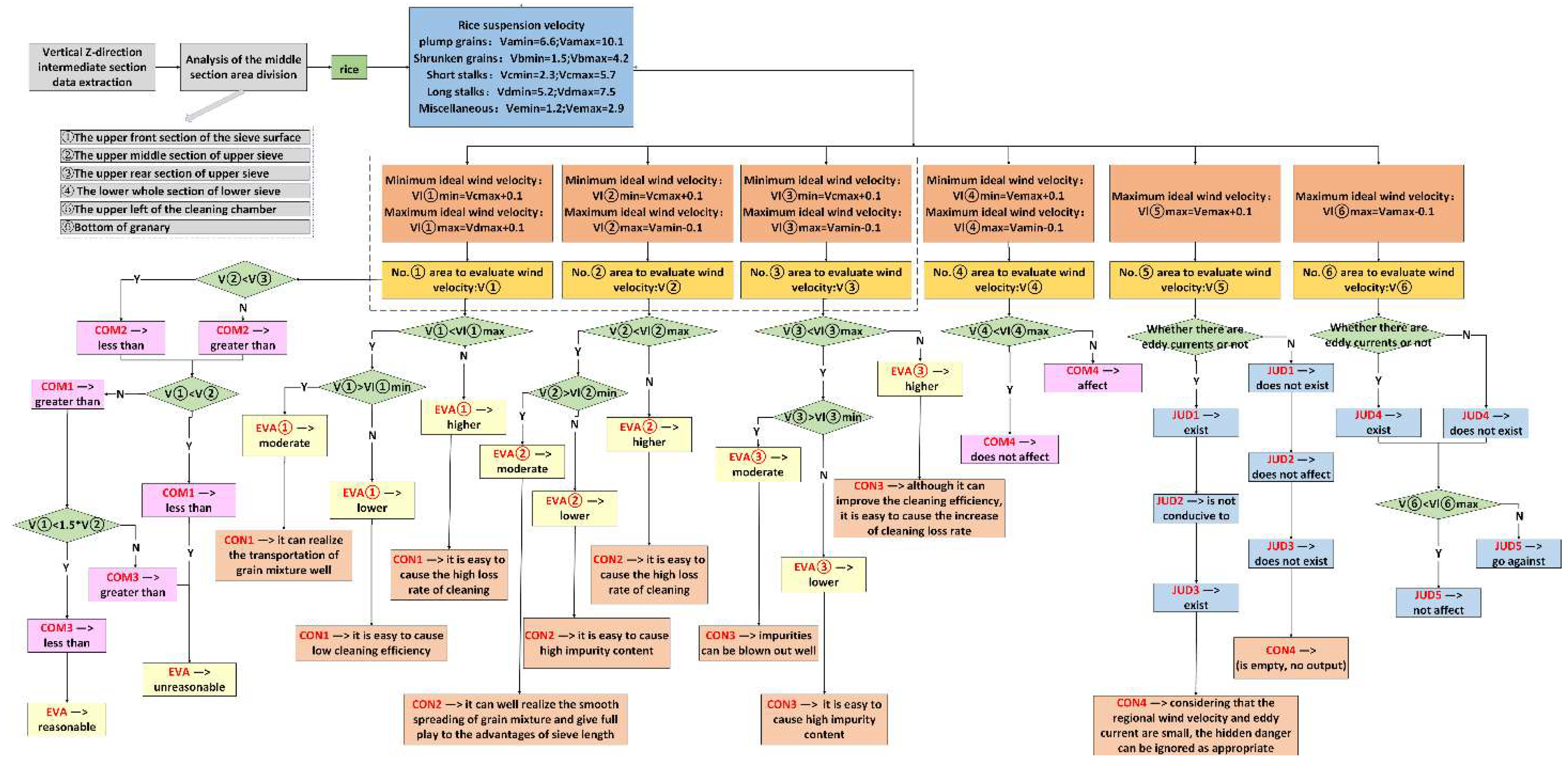
  • Reasoning method for airflow analysis above upper sieve surface of the cleaning chamber
In the process of cleaning and screening, along the length of the upper sieve surface, the distribution of grain mixture presents a law of less in the front, more in the middle and less in the rear. The grains and impurities were easy to accumulate and mix together in the front segment of sieve, and only a small part of the grains closed to the sieve surface and the sieve hole were successfully sorted [22]. As the grain mixture moves along the sieve surface, the material was gradually shaken and blown away, so that the probability of the grain falling into the sieve hole increases. At the end of the sieve, the volume of grain mixture was drastically reduced, the residual impurities were blown out and the remaining grains pass through the cleaning sieve. The distribution of the air flow above the screen surface directly affected the cleaning effect [23,24,25]. Therefore, this paper focused on analyzing the situation of the airflow minimum wind velocity and the minimum suspension velocity of residual impurities, the airflow maximum wind velocity and the minimum suspension velocity of grain in the No.1 area, No.2 area and No.3 area.
  • Reasoning method for airflow analysis under lower sieve surface of the cleaning chamber
Different from the upper sieve surface, the airflow on the lower sieve surface only needed to be evenly distributed and the wind velocity was generally less than the seed suspension velocity [26].
  • Reasoning process for the feed inlet of the cleaning chamber and the grain auger
The inference wind field (in No.5 area and No.6 area) was qualified if there is no vortex or there was vortex but the effective average wind velocity was less than the minimum value of the suspension velocity of the harvested crop.
  • Post-processing reasoning method
The complete process of post-processing reasoning was summarized based on reasoning methods of (2)~(4) above were integrated and combined with the empirical knowledge of sieve airflow analysis of the knowledge base, as shown in Figure 8, and the post-processing conclusion template is shown below:
For the analysis of the velocity field data set near the z= X mm cross-section, it can be seen from the result file data named csv-name that: Above the upper sieve surface, the estimated wind velocity before the sieve is V m/s, and the wind velocity is EVA. The estimated wind velocity in the sieve is V m/s, and the wind velocity is EVA. The wind velocity assessed by the sieve tail is V m/s, and the wind velocity is EVA. The wind velocity before the sieve is COM1 the wind velocity in the sieve, the wind velocity in the sieve is COM2 the wind velocity after the sieve, and the wind velocity before the sieve is COM3 1.5 times the wind velocity in the sieve. The estimated wind velocity of the flow under the lower sieve surface is V m/s, and the wind velocity COM4 the crop particles falling into the grain collection area.
In summary, the airflow distribution on the upper sieve surface is EVA. The wind velocity of the front of the upper sieve is EVA, CON1. The wind velocity of the middle of the upper sieve is EVA, CON2. The wind velocity of the back of the upper sieve is EVA, CON3.
There JUD1 eddy current in the area near the inlet of the cleaning chamber. The estimated regional wind speed is about V m/s, which JUD2 the material transfer. There JUD3 a hidden danger that materials may be involved in eddy current, which causes accumulation and reduces the cleaning efficiency, CON4.
In the area near the grain collection in the cleaning chamber, there JUD4 eddy current, and the regional assessed wind speed is about V m/s, which JUD5 the grain collection work.
Key variable meaning: X is the position coordinate of the section, and the position information of the section. Csv-name indicates the name of the file uploaded by the user, which contains only the file name without the path. V is the estimated wind velocity in the front section above the upper sieve surface (No. 1 area). V is the estimated wind velocity in the middle section above the upper sieve surface (No. 2 area). V is the estimated wind velocity in the rear section above the upper sieve surface (No. 3 area). V is the estimated wind velocity of the whole section under the lower sieve surface (No. 4 area). V is the estimated wind velocity near the inlet of the cleaning chamber (No. 5 area). V is the estimated wind velocity near the grain collection in the cleaning chamber (No. 6 area). EVA is the evaluation of the rationality of the airflow distribution on the upper sieve surface. EVA is the evaluation of the wind velocity in No. 1 area. EVA is the evaluation of the wind velocity in No. 2 area. EVA is the evaluation of wind velocity in No. 3 area. COM1 is the comparison result of wind velocity between No. 1 area and No. 2 area. COM2 is the comparison result of wind velocity between No. 2 area and No. 3 area. COM3 is the comparison result of wind velocity between No. 1 area and 1.5 times No. 2 area. COM4 is the result of the effect of wind velocity on particle fall in No. 4 area. CON1 is the influence result of wind velocity in No. 1 area. CON2 is the influence result of wind velocity in No. 2 area. CON3 is the influence result of wind velocity in region No. 3 area. CON4 is the influence result of eddy in region No. 5 area. JUD1 is the result of the existence or absence of eddy in No. 5 area. JUD2 is the result of the influence of wind velocity area on material transfer in No. 5. JUD3 is the result of the existence or absence of eddy in No. 5 area. JUD4 is the result of the existence or absence of eddy in No. 6 area. JUD5 is the result of influence of wind velocity on material transfer in No. 6 area.

3. Results and Discussion

3.1. Results of Fluid Simulation

The simulation data of all nodes was exported to ASCII format file in order to complete intelligent analysis of the simulation data. Table 3 shows some of the simulation data, in which “x-coordinate”, “y-coordinate”, and “z-coordinate” represent the spatial coordinates where the grid nodes were located, “Velocity Magnitude” represents the magnitude of the wind velocity at the network nodes and “X-Velocity”, “Y-Velocity”, and “Z-Velocity” represent the vector projection of wind velocity in the X, Y, and Z axes. The exported result data storage format was .csv, which provided the basis for the wind velocity evaluation in the object detection area.

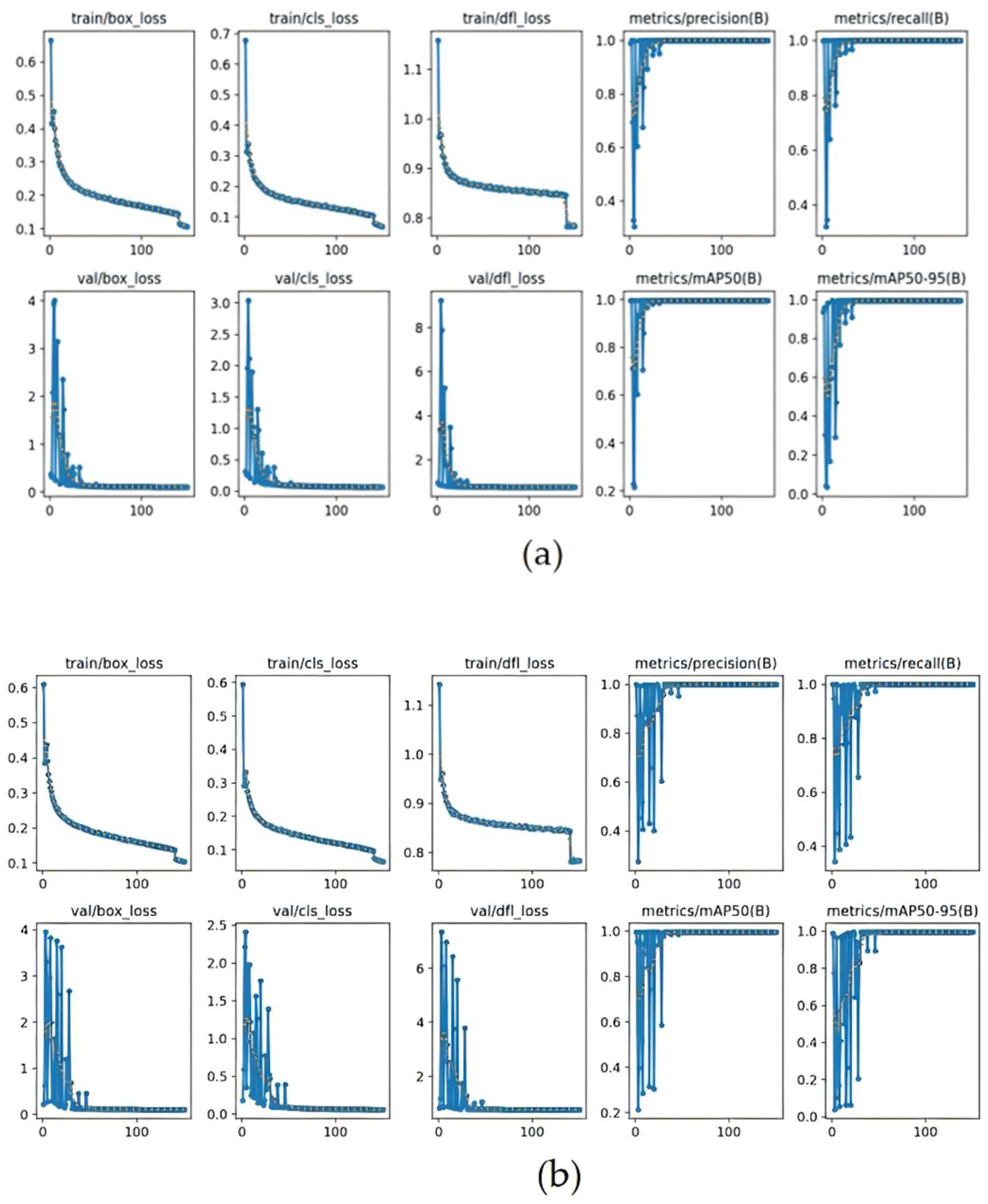
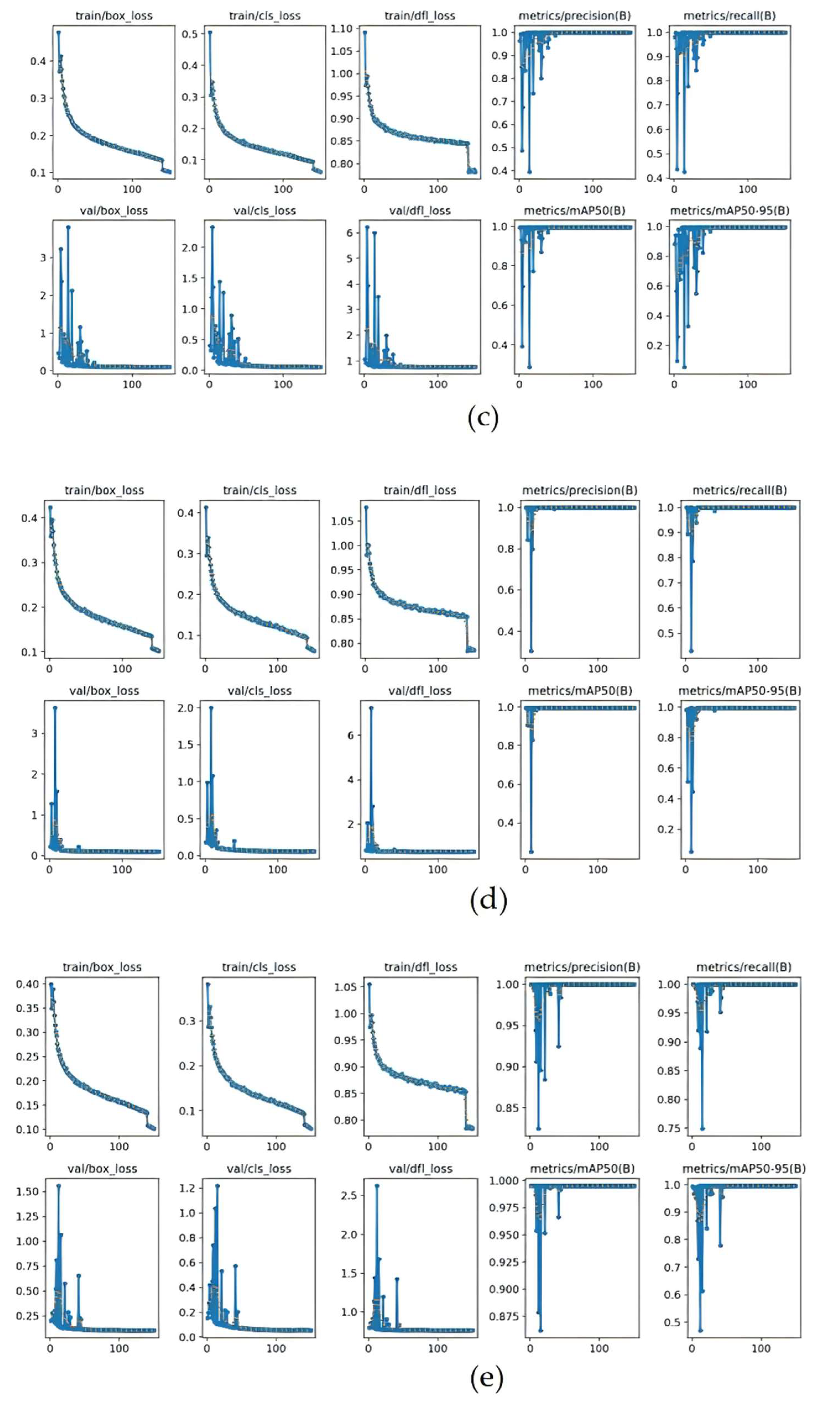
3.2. Performance Evaluation and Training Results of Object Detection Model

Taking the scatter plot of the key cross-section as the training set. The YOLOv8n, YOLOv8s, YOLOv8m, YOLOv8l, and YOLOv8x models were used for training in the same batch. Figure 8 shows the changes in the box_loss, cls_loss, dfl_loss, and mAP values of the five models during the training process. The gradual decrease of box_loss, cls_loss, and dfl_loss indicates that the model’s prediction of the object location was gradually accurate. Respectively, the cls_loss and dfl_loss were used to measure the accuracy of the model for object classification and prediction boxes, and smaller values were more accurate. The mAP value was a performance metric that evaluated the model by considering accuracy and recall, and higher values indicate better detection.
As shown in Figure 9, the box_loss, cls_loss and dfl_loss of each object detection models tended to be balanced after 100 iterations, mAP value gradually increases during the training process and finally tended to be stable. The object detection models could reach convergence after completing all the iterative training, which verified the rationality of the models parameters.
It could be observed that the loss value of each model remained a low state by analyzing the loss curves of the five models on the training dataset and validation dataset. Among them, the cls_loss and dfl_loss of YOLOv8l were slightly smaller than those of the other object detection models. Meanwhile, the YOLOv8l model performed better than the other four models in terms of accuracy and recall, and the convergence curve was smoother and less volatile. Overall, the YOLOv8l model had the best convergence performance.

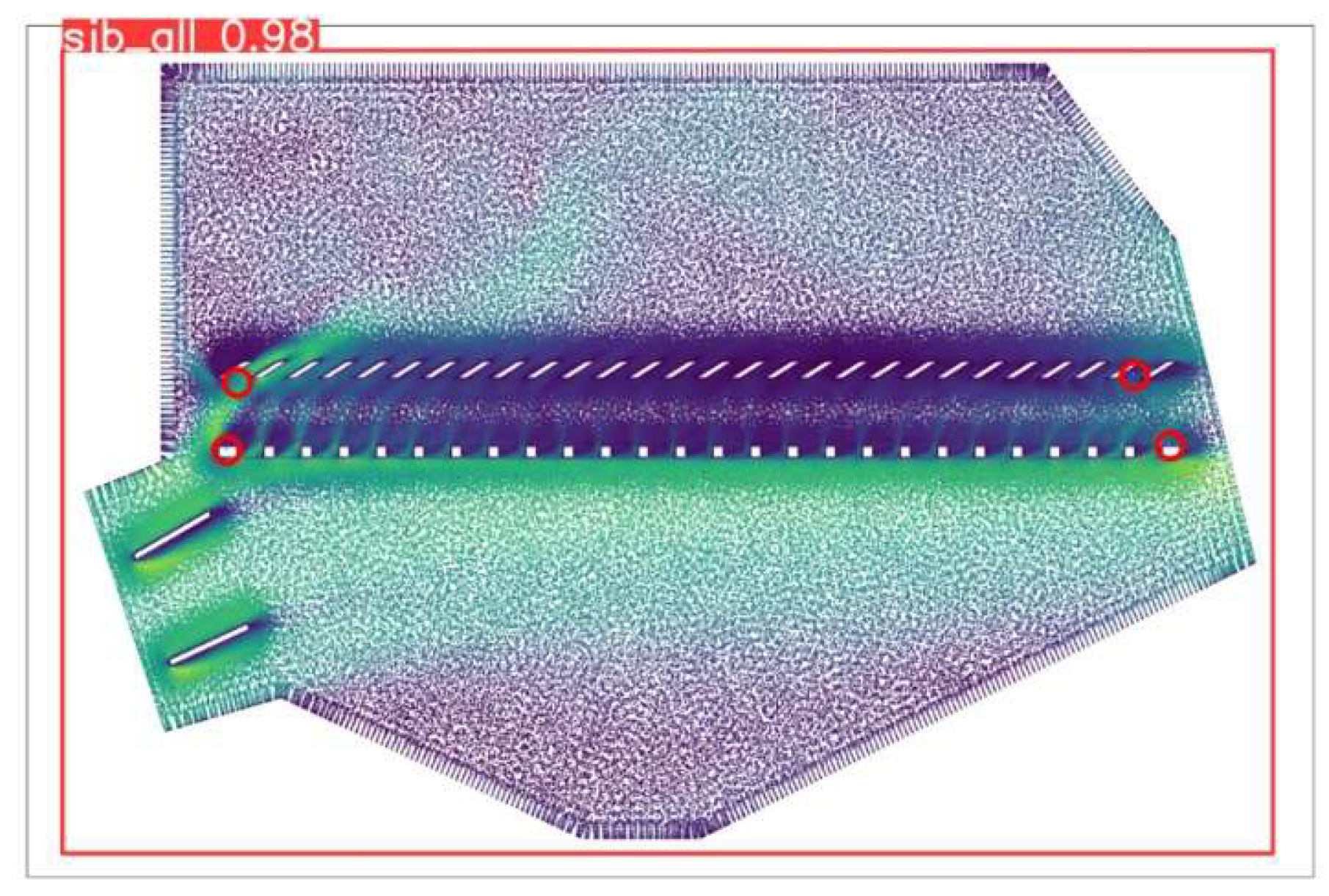
3.3. Testing of Key Point Detection Model

The verification set was selected as the model test object, the scatter plot of the key cross-section perpendicular to the Z-axis direction was selected and the thickness of the data section was 10mm. Then, the trained object detection model was used to identify the key points, Figure 10 is one of the test results.
It could be seen that the error was less than 2.5% between the results from the key point model and manual labeling (in Table 4) . So the model could be applied in practice.

3.4. Reasoning Example of Post-Processing

Zhendao 18 rice was selected as the cleaning plant in this paper. The key areas of the cleaning chamber flow field were divided and the airflow analysis within the regions was carried out based on the knowledge and the post-processing reasoning mechanism. Finally, the airflow distribution characteristics of 6 regions in the cleaning chamber were obtained.
The parameters of Zhendao 18 rice in the knowledge base are : The minimum and maximum values of plump grain suspension velocity are 6.6 m/s and 10.1 m/s, the minimum and maximum values of shrunken grain suspension velocity are 1.5 m/s and 2 m/s, the minimum and maximum values of short stem suspension velocity are 2.3 m/s and 5.7 m/s, the minimum and maximum values of long stem suspension velocity are 5.2 m/s and 7.5 m/s, and the minimum and maximum values of residues suspensions velocity are 1.2 m/s and 2.9 m/s, respectively. The reasoning mechanism based on rules and examples was used to judge the wind velocity and analyse result data in the cleaning chamber, as it is shown:
For the analysis of the velocity field data set near the z=-0.05mm cross-section, it can be seen from the result file data named fluent3_9_all.csv that : Above the upper sieve surface, the estimated wind velocity before the sieve is 4.8580m/s, and the wind velocity is lower. The estimated wind velocity in the sieve is 2.3251m/s, and the wind velocity is lower. The wind velocity assessed by the sieve tail is 4.0239m/s, and the wind velocity is higher. The wind velocity before the sieve is greater than the wind velocity in the sieve, the wind velocity in the sieve is less than the wind velocity after the sieve, and the wind velocity before the sieve is less than 1.5 times the wind velocity in the sieve. The estimated wind velocity of the flow under the lower sieve surface is 6.0693m/s, and the wind velocity does not affect the crop particles falling into the grain collection area.
In summary, the airflow distribution on the upper sieve surface is reasonable. The wind velocity of the front of the upper sieve is lower, it is easy to cause low cleaning efficiency. The wind velocity of the middle of the upper sieve is lower, it is easy to cause high impurity content. The wind velocity of the back of the upper sieve is higher, it is easy to cause the increase of the cleaning loss rate.
There exist eddy current in the area near the inlet of the cleaning chamber. The estimated regional wind speed is about 0.95m/s, which is not conducive to the material transfer. There exist a hidden danger that materials may be involved in eddy current, which causes accumulation and reduces the cleaning efficiency, considering that the regional wind velocity and eddy current are small, the hidden danger can be ignored as appropriate.
In the area near the grain collection in the cleaning chamber, there does not exist eddy current, and the regional assessed wind speed is about 1.1 m/s, which does not affect the grain collection work.
Song Yuying obtained the distribution of air velocity in the cleaning chamber on the 50mm plane under the sieve surface through the analysis of simulation and test results [4], As it is shown: The distribution of air velocity in the cleaning chamber is more uniform at the 50mm plane under the lower sieve surface. After passing through the upper and lower sieve surfaces, the distribution of air velocity has a more obvious change. That is, the velocity in the middle of the front of the sieve and the tail of the sieve surface is larger, and the velocity in the front of the sieve and the rear of the middle of the sieve is smaller. This airflow velocity distribution will lead to the material in front of the sieve can not be effectively separated and is not conducive to the full use of the sieve length to play the advantage of the sieve effect. When the material is transported to the sieve tail, the rapid increase of the wind velocity at the sieve tail may also lead to a high cleaning loss rate.
It could be seen that the reasoning of the wind velocity in the front and tail of the sieve was basically consistent with manual post-processing result, and the conclusions of high cleaning loss rate and low cleaning efficiency were basically consistent with the conclusions of high cleaning loss rate and materials could not be effectively separated in the front of the sieve presented by manual post-processing result. The reasoning result was highly consistent with the manual post-processing result. So the reasoning methods could be used to analyse the wind velocity evaluation of the target detection area.

4. Conclusions

In order to solve the problems that the simulation post-processing of the cleaning chamber almost completely depends on empirical knowledge and the intelligence design is widely used now. The airflow of the cleaning chamber was analyzed based on the object detection algorithm and the reasoning mechanism in this paper. The main conclusions are as follows:
The cls_loss and dfl_loss of YOLOv8l were slightly lower than other models by comparing the loss curves and mAP curves of the training process of the five models of YOLOv8n, YOLOv8s, YOLOv8m, YOLOv8l and YOLOv8x, the YOLOv8l had higher precision and recall than other models, and the convergence curve was smoother and had less large oscillations.
The YOLOv8l model was used to identify the key points of the scatter plot of the key cross-section of the cleaning chamber. The error was less than 2.5% between the key point model identification results and manual marking results.
The key areas of the cleaning chamber flow field were divided through the reasoning mechanism and the key points identified by the YOLOv8l. Then, the airflow analysis within the regions was carried out based on the relevant knowledge and the post-processing reasoning mechanism, and the airflow distribution characteristics of 6 regions in the cleaning chamber were obtained. Zhendao 18 rice was selected as the cleaning object. The results of airflow analysis in 6 regions were obtained: In the upper sieve surface, the wind velocity in the front section is too low which can easily cause low cleaning efficiency, the wind velocity in the middle section is too low which can easily cause high impurity content, and the wind velocity in the tail section is too high which can easily cause high loss rate. There is a vortex in the area near the feed port and the regional wind velocity is about 0.95m/s, which is not conducive to material transmission and is a hidden danger that the material is involved in the eddy and causes accumulation, but the hidden danger is negligible because of the small strength of the eddy current. There is no eddy in the area near the grain collection, the regional wind velocity is about 1.1m/s, which does not affect the grain collection work.

Author Contributions

Conceptualization, Q.L. and R.W.; methodology, Q.L., R.W., Z.W., Y.Y. and X.Z.; software, R.W. and Z.W.; validation, Q.L., R.W. and Z.W.; formal analysis, Q.L. and R.W.; data curation, Z.W., Y.Y. and X.Z.; writing—original draft preparation, Q.L., R.W., Z.W., Y.Y. and X.Z.; writing—review and editing, Q.L., R.W. and Z.W.; All authors have read and agreed to the published version of the manuscript.

Funding

This research was funded by the National Natural Science Foundation of China (61771224) and the Priority Academic Program Development of Jiangsu Higher Education Institutions (No. PAPD2023–87).

Institutional Review Board Statement

Not applicable.

Data Availability Statement

The data that support the findings of this study are available upon request from the corresponding author. The data are not publicly available due to privacy or ethical restrictions.

Acknowledgments

We gratefully acknowledge our colleagues at the School of Agricultural of Jiangsu University for their assistance. All the authors acknowledge and thank their respective institutes and universities for providing library facilities.

Conflicts of Interest

The authors declare no conflicts of interest.

References

  1. Helena, M.; Simon, D. The cultural transmission of tacit knowledge. Journal of the Royal Society Interface, 2022, 19, 20220238.
  2. Mingjun, C. Developing Simulation System of FEA Based on Visual Studio and Python Language. Master’s Thesis, Qingdao University of Technology, Qingdao, 2015.
  3. Wenbin, L. Construction of CAE post processing system for key parts of threshing device of combine harvester. Master’s Thesis, Jiangsu University, Zhenjiang, 2021.
  4. Yuying, S. The Platform Construction of Combine Harvester Cleaning Flow Field CAE PostProcessing and Cleaning Device Optimization. Master’s Thesis, Jiangsu University, Zhenjiang, 2021.
  5. Ante, T.; Wenbin, S.G. Auto CAE analytical system for the strength and modal analysis on the vehicle’s sub-frame. Journal of Machine Design, 2019, 36, 13-19.
  6. Che, J.; Zhang, Y.; Yang, Q.; Yuting, H. Research on person re-identification based on posture guidance and feature alignment. Multimedia Systems, 2023, 29, 763-770. [CrossRef]
  7. Mochen, L.; Zhenyuan, C.; Mingshi, C.; Qinglu, Y.; Jinxing, W.; Huawei, Y. Red Ripe Strawberry Recognition and Stem Detection Based on Improved YOLOv8-Pose. Transactions of the Chinese Society for Agricultural Machinery, 2019, 54, 244-251.
  8. Zhongfeng, G.; Junchi, L.; Junlin, Y. Weld recognition based on key point detection method. Transactions of the China Welding Institution, 2019, 45, 88-93+134.
  9. Lu, G.; Xiaodong, L.; Yufeng, W.; Zhen, Z. Control Decision of Equipment Health State based on Big Data Reasoning. Air &Space Defense, 2023, 6, 85-94.
  10. Yu, Z.; Ziming, K.; Cong, H.; Shaokai, K. Fault diagnosis of belt conveyor drive system based on RBR + CBR dual reasoning. Journal of Mechanical & Electrical Engineering, 2023, 40, 1785-1793.
  11. Cong, L.; Beibei, F.; Wenwei, Y. Research on Rapid Product Design Based on Reasoning Model. Metrology & Measurement Technology, 2018, 45, 23-26.
  12. Mengqi, C.; Rong, Q.; Weiguo, F. Case-based reasoning system for fault diagnosis of aero-engines. Expert Systems with Applications, 2022, 202, 117350.
  13. Lao, S.I.; Choy, K.L.; Ho, G.T.; Richard, C.M.; Tsim, Y.C.; Poon, T.C. Achieving quality assurance functionality in the food industry using a hybrid case-based reasoning and fuzzy logic approach. Expert Systems with Applications, 2012, 39, 5251-5261. [CrossRef]
  14. Yi, C.; Zhuo, Y.; Zhenxiang, H.; Weihong, S.; Liang, H. A Decision-Making System for Cotton Irrigation Based on Reinforcement Learning Strategy. Agronomy-Basel, 2024, 14, 11.
  15. Chengang, D.; Guodong, D. An enhanced real-time human pose estimation method based on modified YOLOv8 framework. Scientific Reports, 2024, 14, 8012.
  16. Jianhua, Z.; Review of commercial CFD software. Journal of Hebei University of Science and Technology, 2005, 26, 160-165.
  17. Zhenwei, L.; Lizhang, X.; Josse, D.B.; Yaoming, L.; Wouter, S. Optimisation of a multi-duct cleaning device for rice combine harvesters utilising CFD and e02xperiments. Biosystems Engineering, 2020, 190, 25-40.
  18. Peng, L.; Chengqian, J.; Tengxiang, Y.; Man, C.; Youliang, N.; Xiang, Y. Design and Experiment of Multi Parameter Adjustable and Measurable Cleaning System. Transactions of the Chinese Society for Agricultural Machinery, 2020, 51, 191-201.
  19. Jaehyeop, C.; Chaehyeon, L.; Donggyu, L.; Heechul, J. SalfMix:A Novel Single Image-Based Data Augmentation Technique Using a Saliency Map. Sensors, 2021, 21, 8444.
  20. Matheus, F.G.; Igor, R.F.; Rafael, K.; Franklin, C.F. System of Counting Green Oranges Directly from Trees Using Artificial Intelligence. AgriEngineering, 2023, 5, 1813-1831.
  21. Bochuan, D.; Zhenwei, L.; Yongqi, Q.; Zhikang, Y.; Jiahao, Z. Improving Cleaning Performance of Rice Combine Harvesters by DEM–CFD Coupling Technology. Agriculture-Basel, 2022, 12, 1457.
  22. Xiaoyu, C.; Lizhang, X.; Yixin, S.; Zhenwei, L.; En, L.; Yaoming, Li. Development of a cleaning fan for a rice combine harvester using computational fluid dynamics and response surface methodology to optimise outlet airflow distribution. Biosystems Engineering, 2020, 192, 232-244.
  23. Junwei, C.; Zengde, H.; Zirui, Z.; Fuping, H.; Bangxing, G.; Tiansheng, S.; Xiaodong, Q. Experiments and Analysis about Airflow Distribution over Oscillating Sieve of Grain Combine Harvester. Agricultural Engineering, 2015, 5, 1-4+14.
  24. Fang, C.; Jun, W. Test Study on the Flow Field Above Surface of the Air-and-Screen Cleaning Mechanism. Transactions of the Chinese Society of Agricultural Engineering, 1999, 15, 55-58.
  25. Guohua, D.; Yi, Y. The Influence of Airstream Distribution Along a Sieve on The Separation of Grain Mixture. Transactions of the Chinese Society for Agricultural Machinery, 1982, No.3, 16-28.
  26. Lizhang, X.; Yang, L.; Xiaoyu, C.; Guimin, W.; Zhenwei, L.; Yaoming, L.; Baijun, L. Numerical simulation of gase-solid two-phase flow to predict the cleaning performance of rice combine harvesters. Biosystems Engineering, 2020, 19, 11-24.
Figure 1. The technical route of intelligent analysis of wind field characteristics in cleaning chamber.
Preprints 145196 g001
Figure 2. Cleaning device. (a) is combine harvester cleaning device, (b) is simplified geometric model of cleaning device, a is air inlet of the cleaning chamber, b is upper airflow guide plate, c is lower airflow guide plate, d is louver sieve, e is mesh sieve, f is air outlet of the cleaning chamber.
Preprints 145196 g002
Figure 3. Example diagram of wall classification. (a) shows air outlet of the cleaning chamber, (b) shows air inlet of the cleaning chamber, (c) shows little_wall of the cleaning chamber, (d) shows middle_wall of the cleaning chamber, (e) shows big_wall of the cleaning chamber.
Preprints 145196 g003
Figure 4. Example diagram of grid partitioning. (a) is mesh sieve local, (b) is louver sieve local, (c) is cleaning chamber wall local, (d) is cleaning chamber overview.
Preprints 145196 g004
Figure 5. Key cross-section scatter and key point position diagram. (a) shows slice thickness 100mm, (b) shows slice thickness 20mm, (c) shows slice thickness 10mm, (d) shows slice thickness 2mm, (e) shows example diagram of key point location, ① is the front endpoint of the upper sieve surface, ② is the rear endpoint of the upper sieve surface, ③ is the front endpoint of the lower sieve surface, ④ is the rear endpoint of the lower sieve surface.
Preprints 145196 g005
Figure 6. Schematic diagram of division of regional locations.
Preprints 145196 g006
Figure 7. Reasoning process of flow field detection area division in cleaning chamber.
Preprints 145196 g007
Figure 8. Process oriented conclusion inference in post-processing.
Preprints 145196 g008
Figure 9. The loss curves and mAP curves of the model training process. (a) shows the loss curves and mAP curves of YOLOv8n model training process, (b) shows the loss curves and mAP curves of YOLOv8s model training process, (c) shows the loss curves and mAP curves of YOLOv8m model training process, (d) shows the loss curves and mAP curves of YOLOv8l model training process, (e) shows the loss curves and mAP curves of YOLOv8x model training process.
Preprints 145196 g009aPreprints 145196 g009b
Figure 10. Test results of yolov8l-pose model.
Preprints 145196 g010
Table 1. Key parameters of the cleaning chamber for 12 commonly used machine models.
Machine Model Clearing chamber length (m) Clearing chamber height (m) Upper sieve length (m) Lower sieve length (m)
1 4LBZ-145 0.8755 0.5736 0.680 0.700
2 4LZ-5G 1.0180 0.6065 0.800 0.800
3 4LZY-1.5 1.1109 0.8520 0.800 0.880
4 DFQX-3 1.1289 0.8295 0.760 0.820
5 ZKB-5 1.3447 1.0226 1.018 1.018
6 4LZ-7N 1.1026 0.9125 0.860 0.860
7 Fengshou-3.0 1.2380 0.9270 1.000 1.000
8 4LZB-105 1.0434 0.6586 0.820 0.860
9 4LZ-2.5 1.2828 0.9289 0.800 1.000
10 4LZ-1.0 0.9872 0.6262 0.680 0.700
11 4LQ-2.5 1.0093 0.9706 0.800 1.000
12 DF-1.5 1.0455 0.758 0.720 0.820
Table 2. Local size parameter settings.
Name Local size (mm)
Little_wall 2.5
Middle_wall 5
Out_wall 5
In_wall 5
Big_wall 10
Table 3. Local data of simulation results for model.
Node number X-coordinate Y-coordinate Z-coordinate Velocity-magnitude X-velocity Y-velocity Z-velocity
1 0.726608 0.541836 0.028558 2.734538 2.509488 1.084060 -0.055024
2 0.727234 0.542215 0.027279 2.845202 2.604854 1.141396 -0.068198
3 0.726470 0.541786 0.025921 2.741601 2.516079 1.084341 -0.082012
4 0.725315 0.541097 0.026017 2.552531 2.356438 0.975582 -0.078499
5 0.724714 0.540719 0.027356 2.446941 2.264678 0.921151 -0.067528
6 0.725436 0.541144 0.028614 2.552805 2.352640 0.987235 -0.056994
7 0.725107 0.541634 0.028590 3.600152 3.293722 1.452340 -0.052900
8 0.726143 0.542751 0.028582 3.963142 3.616092 1.620895 -0.050203
9 0.725658 0.542753 0.028570 4.131888 3.763608 1.704038 -0.049944
10 0.724466 0.541147 0.027393 3.527243 3.230571 1.414100 -0.068024
11 0.726772 0.543075 0.027260 3.987315 3.638826 1.628794 -0.065586
12 0.726282 0.543429 0.027800 4.351541 3.967640 1.785891 -0.060108
13 0.726326 0.543033 0.026680 4.101440 3.738727 1.684544 -0.073610
14 0.725576 0.543874 0.027660 4.855009 4.404069 2.041239 -0.059116
15 0.726172 0.542234 0.025922 3.594810 3.281631 1.464883 -0.081411
16 0.725101 0.541493 0.026015 3.547387 3.246728 1.426615 -0.083277
17 0.724560 0.541713 0.026747 3.839289 3.501243 1.572507 -0.074493
18 0.759107 0.536109 0.020085 2.331602 2.045293 1.111270 -0.012298
19 0.759383 0.535617 0.020086 2.729842 2.324775 1.429933 -0.039978
20 0.758751 0.535255 0.021306 2.685071 2.298429 1.387512 -0.022273
Table 4. The recognition results of YOLOv8l model are compared with the manual annotation results.
Model identification coordinates(m) manual marking coordinates(m) Error
1 (0.12557, 0.41514) (0.12673, 0.41875) (0.92%, 0.86%)
2 (0.95780, 0.41309) (0.96078, 0.41875) (0.31%, 1.35%)
3 (0.12993, 0.35823) (0.12988, 0.35041) (0.04%, 2.23%)
4 (0.96176, 0.35908) (0.98225, 0.35041) (2.08%, 2.47%)
Note: The coordinate origin of the model recognition is consistent with manual marking coordinates, that is, the coordinate origin of the model(the coordinate origin is in the lower left corner of the model).
Disclaimer/Publisher’s Note: The statements, opinions and data contained in all publications are solely those of the individual author(s) and contributor(s) and not of MDPI and/or the editor(s). MDPI and/or the editor(s) disclaim responsibility for any injury to people or property resulting from any ideas, methods, instructions or products referred to in the content.
Copyright: This open access article is published under a Creative Commons CC BY 4.0 license, which permit the free download, distribution, and reuse, provided that the author and preprint are cited in any reuse.
Prerpints.org logo

Preprints.org is a free preprint server supported by MDPI in Basel, Switzerland.

Subscribe

Disclaimer

Terms of Use

Privacy Policy

Privacy Settings

© 2026 MDPI (Basel, Switzerland) unless otherwise stated