Submitted:
06 January 2025
Posted:
07 January 2025
You are already at the latest version
Abstract
This study introduces an AI-based approach to planning sanitary facilities in buildings, with a focus on Long Short-Term Memory (LSTM) neural networks. By examining factors like occupancy patterns, daily fluctuations, and building-specific characteristics, the model delivers datadriven guidance for fixture allocation. Validation was carried out using empirical data from a Singaporean office building, resulting in strong predictive performance and improved operational efficiency. The LSTM model surpassed traditional methods, with a 39.26% boost in Mean Absolute Percentage Error (MAPE) over queueing theory. In a real-world scenario, its predictions were within 2.63%–4.76% of actual needs, whereas prescriptive codes deviated by 12.07%–19.05%. Sensitivity analysis showed that total occupancy, time of day, and gender ratio exerted the greatest influence, enabling gender-specific recommendations. The findings also indicate a potential 15% cut in overall fixtures with no compromise in service quality, providing considerable cost and space savings. By uniting advanced computational modeling with real data, this research demonstrates how AI can elevate sanitary facility planning toward evidence-based decision-making, efficient resource use, and higher user satisfaction. The results may influence policy, regulatory standards, and performance oriented design in contemporary buildings.
Keywords:
1. Introduction
1.1. Background on Sanitary Facility Planning Challenges
1.2. Context of the Singapore Office Building Study
1.3. The Role of Artificial Intelligence in Facility Planning
1.4. Objectives and Contributions of the Study
- Build a predictive model that accounts for time-based, demographic, and environmental factors
- Compare AI-based forecasts against traditional methods
- Pinpoint critical factors shaping restroom usage
- Illustrate practical benefits of the model in a working environment
2. Literature Review
2.1. Prescriptive Codes – Comparative Analysis of International Toilet Standards
- -
- Rely on static models that may miss flexible work hours or variable occupancy [11]
- -
- Struggle with unique cultural practices or peak events [1]
- -
- Risk over- or under-providing, leading to cost burdens or user frustration [12]
- -
- Often refer to outdated assumptions, overlooking workplace shifts like remote work or evolving gender norms [13]
2.2. Queueing Theory Models for Toilet Facilities
2.3. Applications of Machine Learning in Facilities Management
- -
- -
- -
- Restroom Optimization: Lokman et al. [20] used sensor data to optimize cleaning schedules, hinting at wider possibilities for fixture planning.
- -
2.4. Gaps in Current Approaches
3. Methodology
3.1. Overview of Proposed Machine Learning Approach
- Data Collection and Preprocessing – Compiling both empirical and synthetic datasets to reflect a range of usage scenarios.
- Feature Engineering – Identifying and extracting key variables, including occupancy levels, gender distribution, and temporal factors.
- Model Development and Training – Designing and refining the LSTM architecture using the preprocessed dataset.
- Hyperparameter Tuning – Systematically optimizing the model configuration to elevate predictive accuracy.
- Performance Evaluation – Measuring the final model’s performance against standard methods like queueing theory.
3.2. Data Collection and Preprocessing
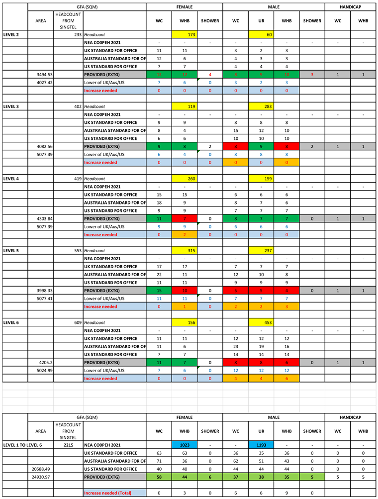
3.2.1. Original Data from Singtel Report
- -
- Occupancy Records: Verified occupant counts (male and female) spanning Floors 2–6, enabling thorough gender-based analysis.
- -
- Facility Inventories: Comprehensive listings of toilets (WCs), urinals (URs), wash hand basins (WHBs), and showers, captured across floors.
- -
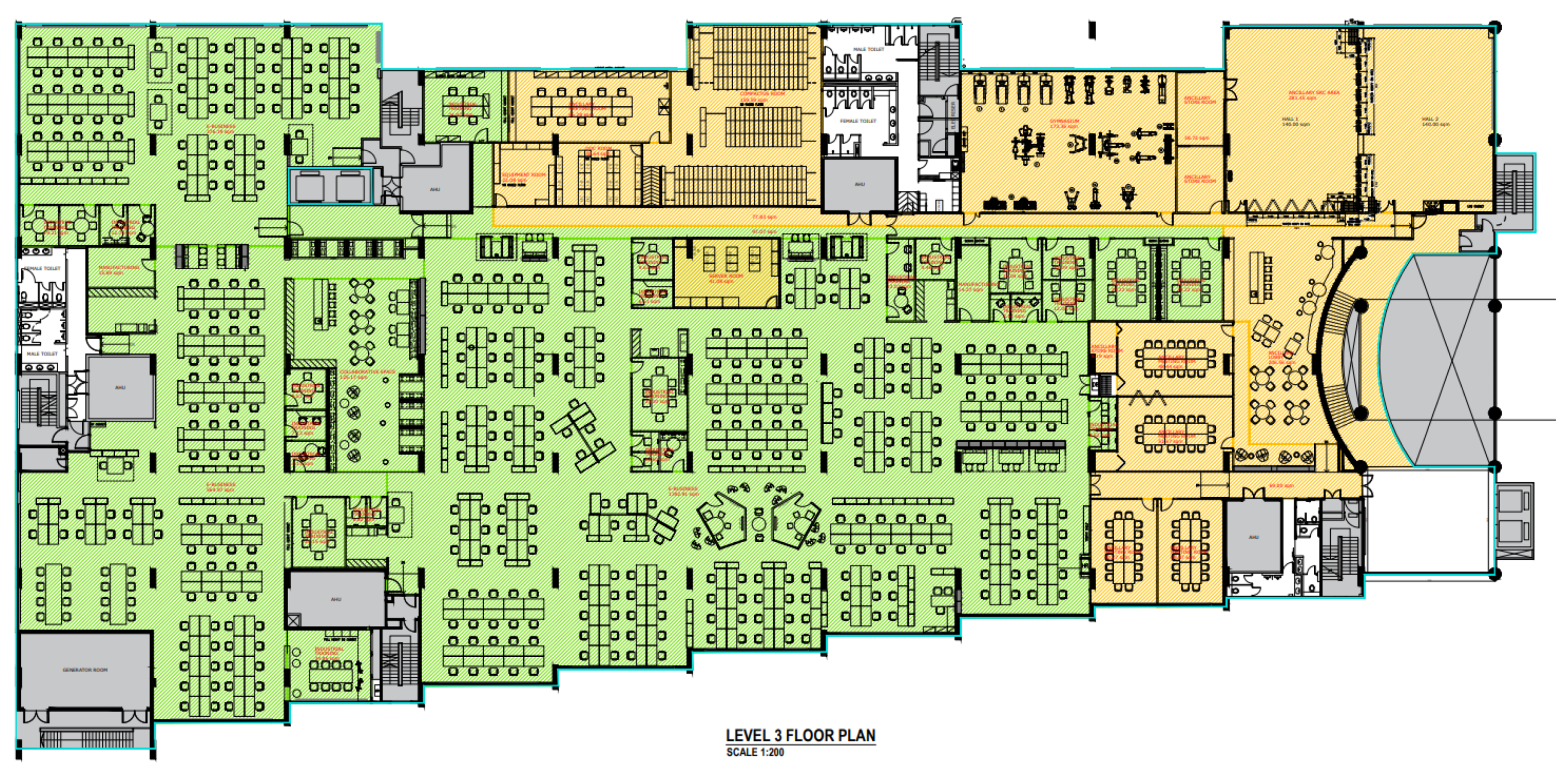
- Floor Plans: Architectural blueprints to factor in spatial layout, accessibility, and fixture distribution.
- -
- Usage Assumptions: Behavioral metrics derived from the World Toilet Organization, such as average toilet visits (four per occupant per day) and service durations (3 minutes per visit for females, 1.5 minutes for males).
- -
- International Benchmarks: Baseline comparisons grounded in sanitary provisions outlined by the UK, Australia, and the United States.
- -
- Population Increases – Occupant surges of 10%, 20%, 30%, and 40%, representing various high-demand situations.
- -
- Reduced Utilization – Occupancy dropping to 85% of the baseline, simulating lower-demand environments.
3.2.2. Scenario Variations
- -
- Population Increases: Gradual escalations of 10%, 20%, 30%, and 40% to mirror busier periods.
- -
- Reduced Utilization: Scaling back to 85% occupancy to capture off-peak conditions.
3.2.3. Summary of Current Facilities
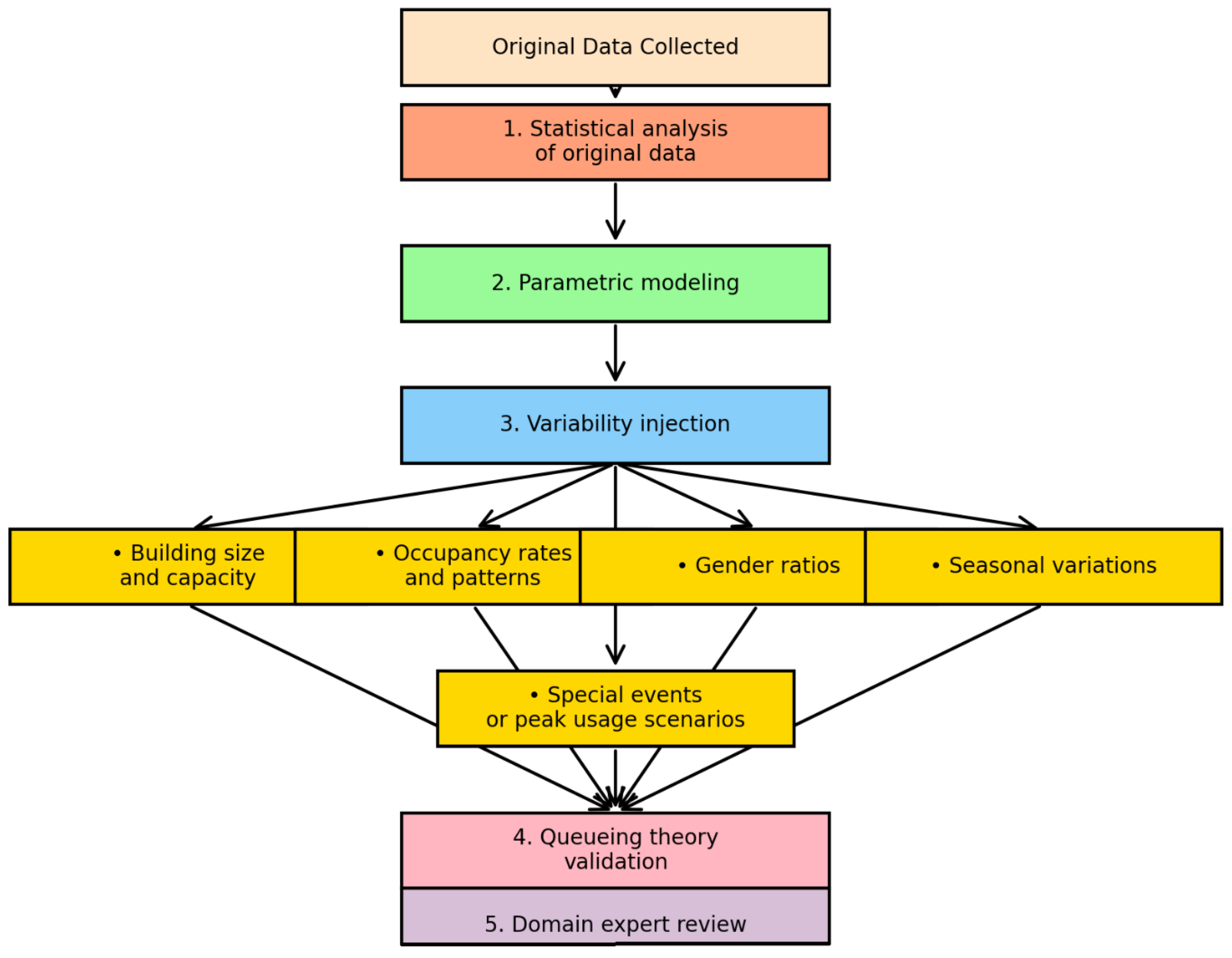
3.2.4. Data Enhancement and Scenario Testing
- 1.
- Scenario Variability
- -
- Occupancy Adjustments: Incremental increases of 10%–40% and a cutback to 85% baseline to emulate extremes of usage
- -
- Demographic Ratios: Shifts in the male-to-female ratio to gauge differential fixture requirements
- -
- Temporal Patterns: Inclusion of seasonal and time-of-day fluctuations
- -
- Event-Based Surges: Additional bursts in occupancy during conferences, meetings, or other peak activity windows
- 2.
- Validation with Queueing Models
- -
- M/M/c and M/G/c queueing frameworks were applied to confirm that the synthetic data mirrored realistic operational patterns in queue lengths and waiting times.
- 3.
- Expert Review
- -
- Facility management practitioners reviewed these extended scenarios to validate that the adjustments stayed true to real-life building dynamics.
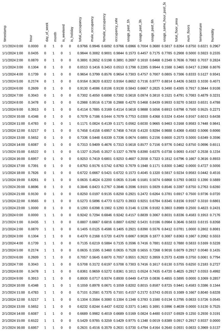
3.3. Feature Selection and Engineering
- -
- Temporal Features: Hourly/daily indicators and seasonal markers, with flags for weekends and holidays
- -
- Occupancy Features: Total occupant count, gender ratio, and occupancy change rate
- -
- Environmental Features: Weather metrics (temperature and humidity) to control for external factors
- -
- Building Characteristics: Floor area, layout constraints, and total floors
- -
- Event Features: Indicators for specific events, coupled with estimates of attendee numbers
3.4. Machine Learning Model Development
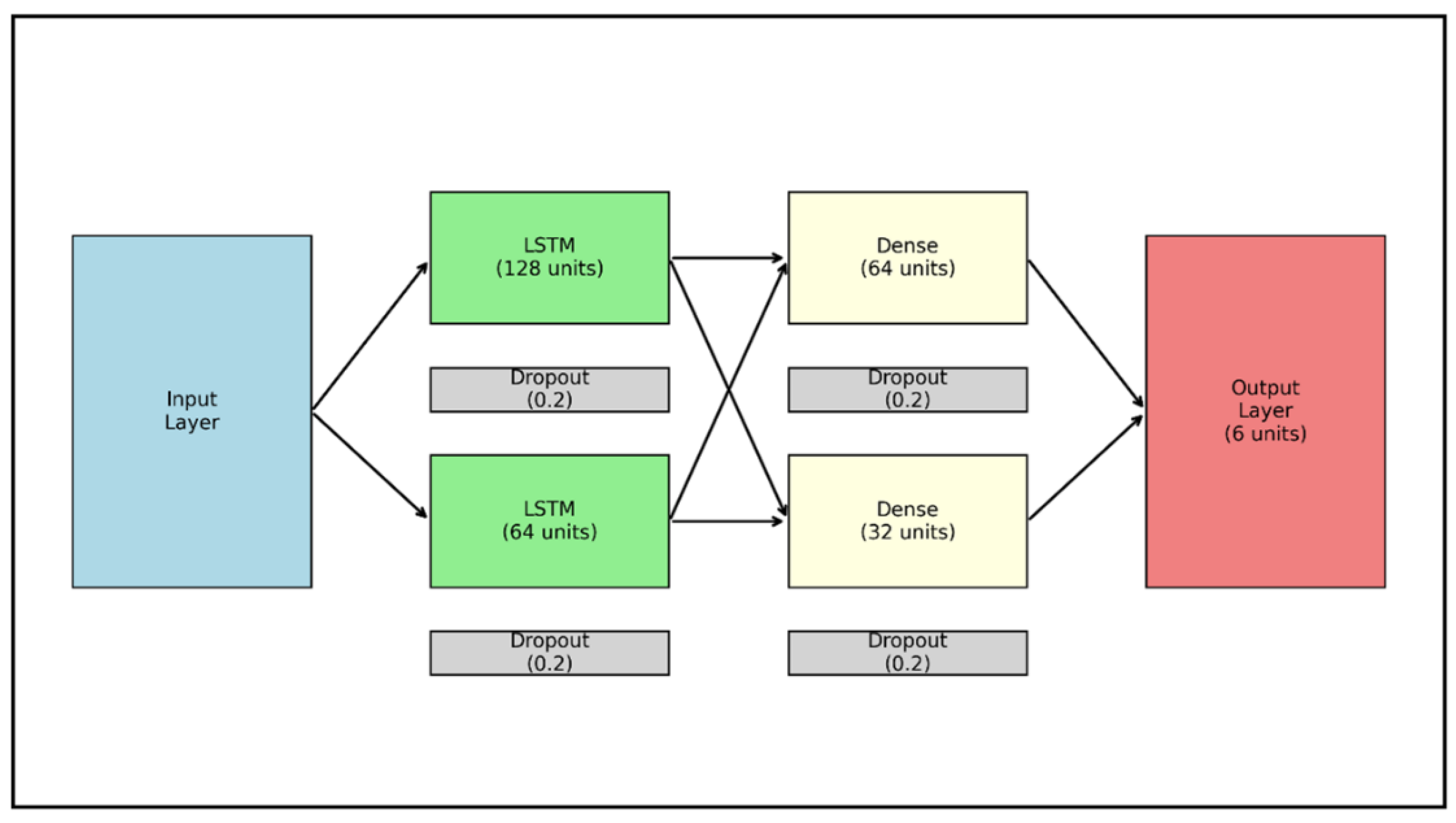
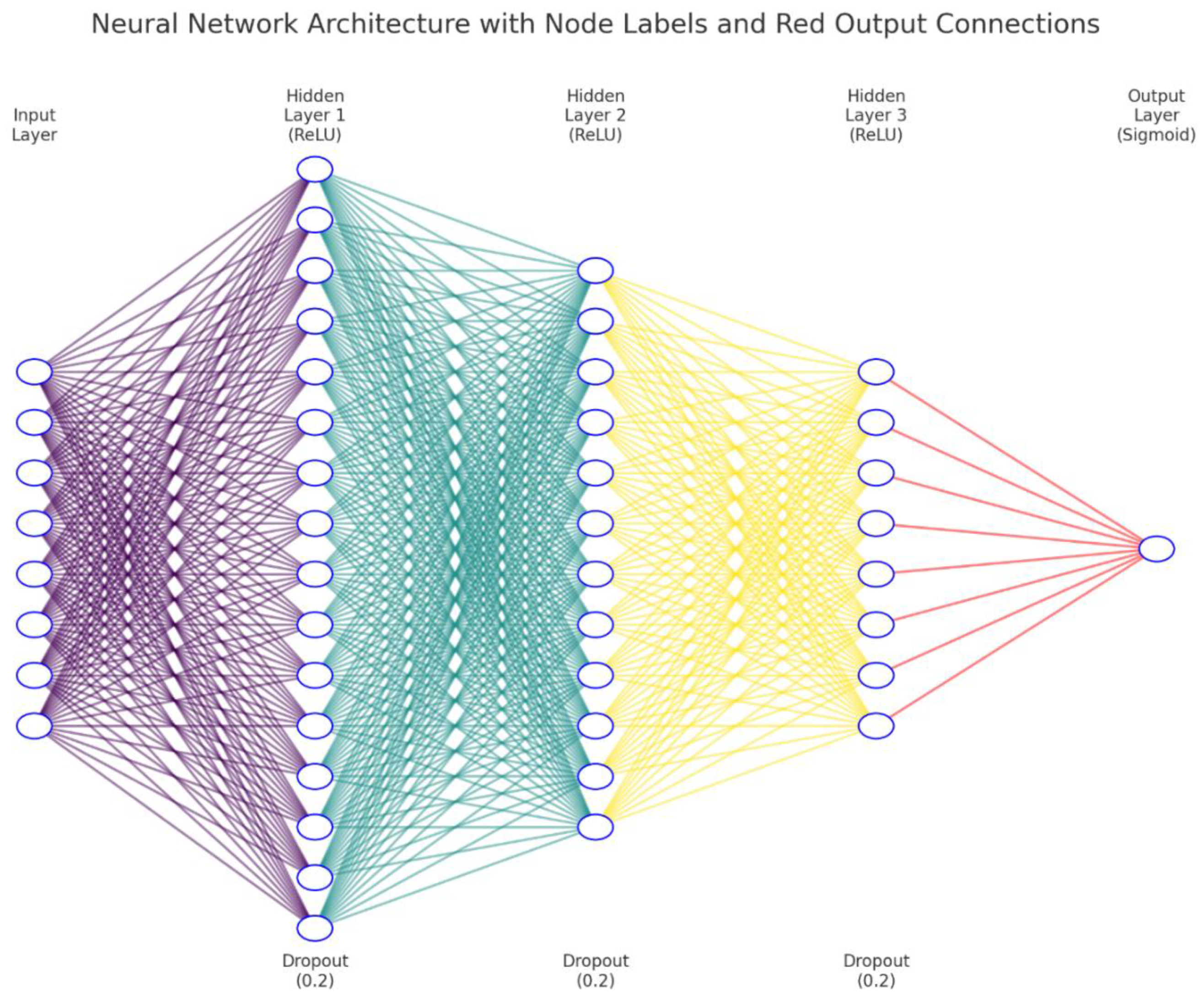
3.4.1. Model Architecture
- 1.
- Input Layer
- -
- Receives the refined features outlined in Section 3.3.
- 2.
- LSTM Layers
- -
- Two stacked LSTM layers with 128 and 64 units, respectively, designed to identify both short-term fluctuations and longer-term usage cycles.
- 3.
- Dense Layers
- -
- Two fully connected layers with 64 and 32 units, each leveraging ReLU activa tion. The outputs from the LSTM stack are combined with non-time-based features, providing a holistic view of restroom demand.
- 4.
- Output Layer
- -
- A final dense layer featuring six units—predicting the number of toilets, urinals, and washbasins needed for both female and male occupants—using a linear activation function.
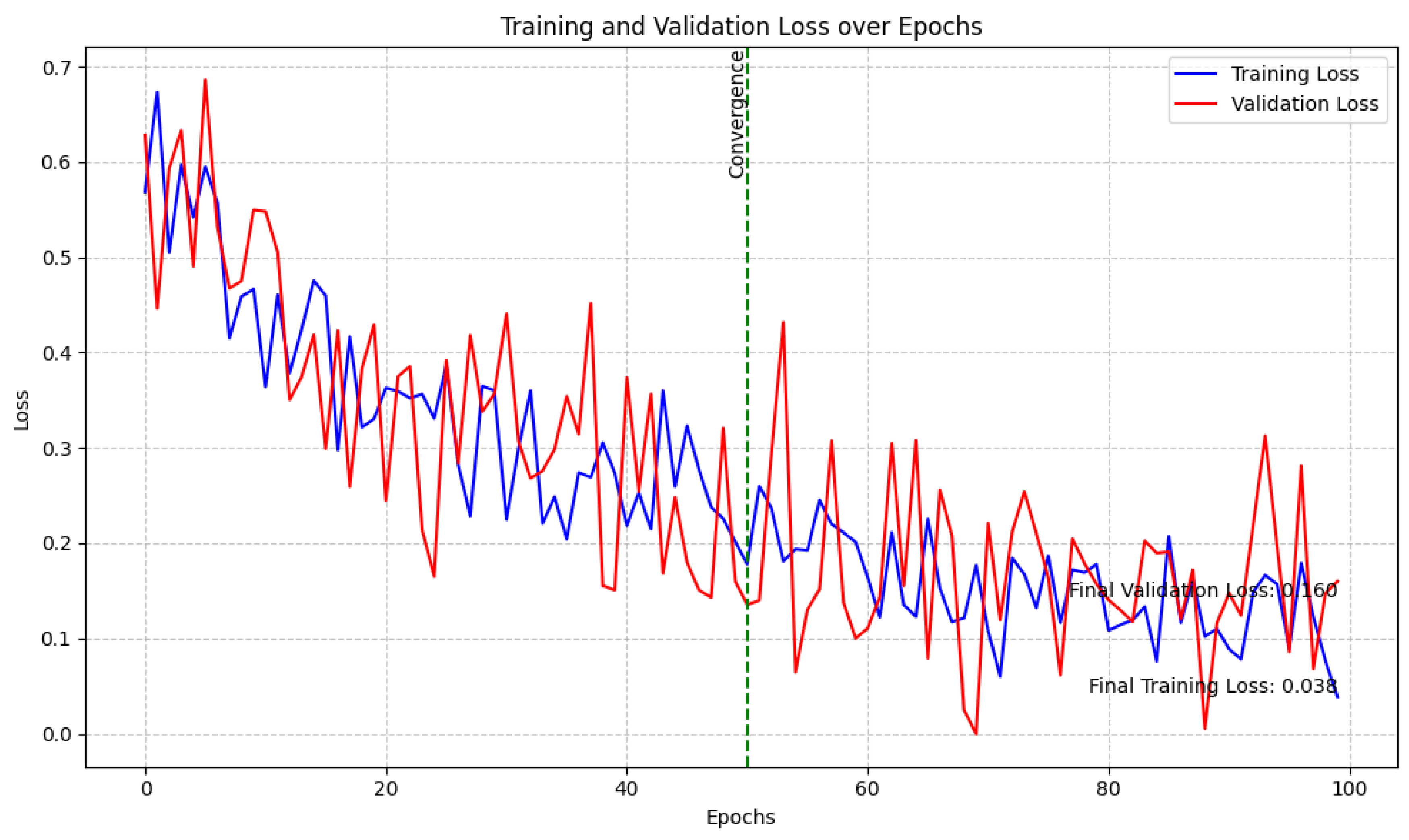
3.4.2. Training Process
- 1.
- Data Partitioning
- -
- 70% of the data was assigned for training, 15% for validation, and the final 15% for testing.
- 2.
- Batch Training
- -
- Mini-batches of size 64 were employed for 100 epochs, facilitating steady gradient updates and helping to deter overfitting.
- 3.
- Early Stopping
- -
- Training was halted once validation loss failed to improve for 10 consecutive epochs, a safeguard against excessive overfitting.
- 4.
- Adaptive Learning Rate
- -
- The learning rate was halved whenever the validation loss showed no progress for 5 straight epochs, helping stabilize training.
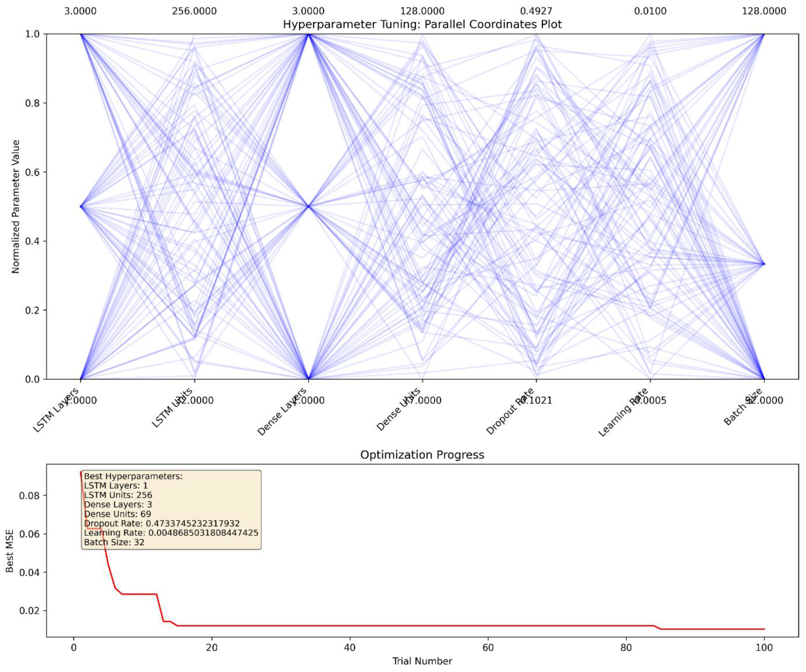
3.4.3. Hyperparameter Tuning
- -
- Number of LSTM Layers (ranging from 1–3)
- -
- Units in Each Layer (32–256)
- -
- Number of Dense Layers (1–3)
- -
- Dropout Rates (0.1–0.5)
- -
- Learning Rates (0.0001–0.01)
- -
- Batch Sizes (32–128)
3.5. Performance Evaluation Metrics
- 1.
- Mean Squared Error (MSE)
- -
- Evaluates the average of squared deviations between predictions and actual values.
- 2.
- Root Mean Squared Error (RMSE)
- -
- The square root of MSE, offering a direct measure of prediction accuracy in original units.
- 3.
- Mean Absolute Error (MAE)
- -
- The average of absolute differences between predictions and observations.
- 4.
- Mean Absolute Percentage Error (MAPE)
- -
- Reflects relative accuracy by expressing errors as a percentage of observed values.
- 5.
- R-squared (R²)
- -
- Indicates how much variance in the target variable is explained by the model.
- 6.
- Queue Length Accuracy (QLA)
- -
- Compares predicted queue lengths (Q_pred) with actual queue lengths (Q_actual).
- 7.
- Waiting Time Accuracy (WTA)
- -
- Measures the precision of predicted waiting times (W_pred vs. W_actual).
- 8.
- Fixture Utilization Accuracy (FUA)
- -
- Compares predicted fixture utilization rates (U_pred) to actual rates (U_actual).
- 9.
- Peak Demand Accuracy (PDA)
- -
- Assesses the model’s ability to anticipate the highest usage periods accurately.
- 10.
- Gender-Specific Accuracy (GSA)
- -
- Evaluates how closely predicted fixture counts for each gender match reality (F_pred_gender vs. F_actual_gender).
4. Results
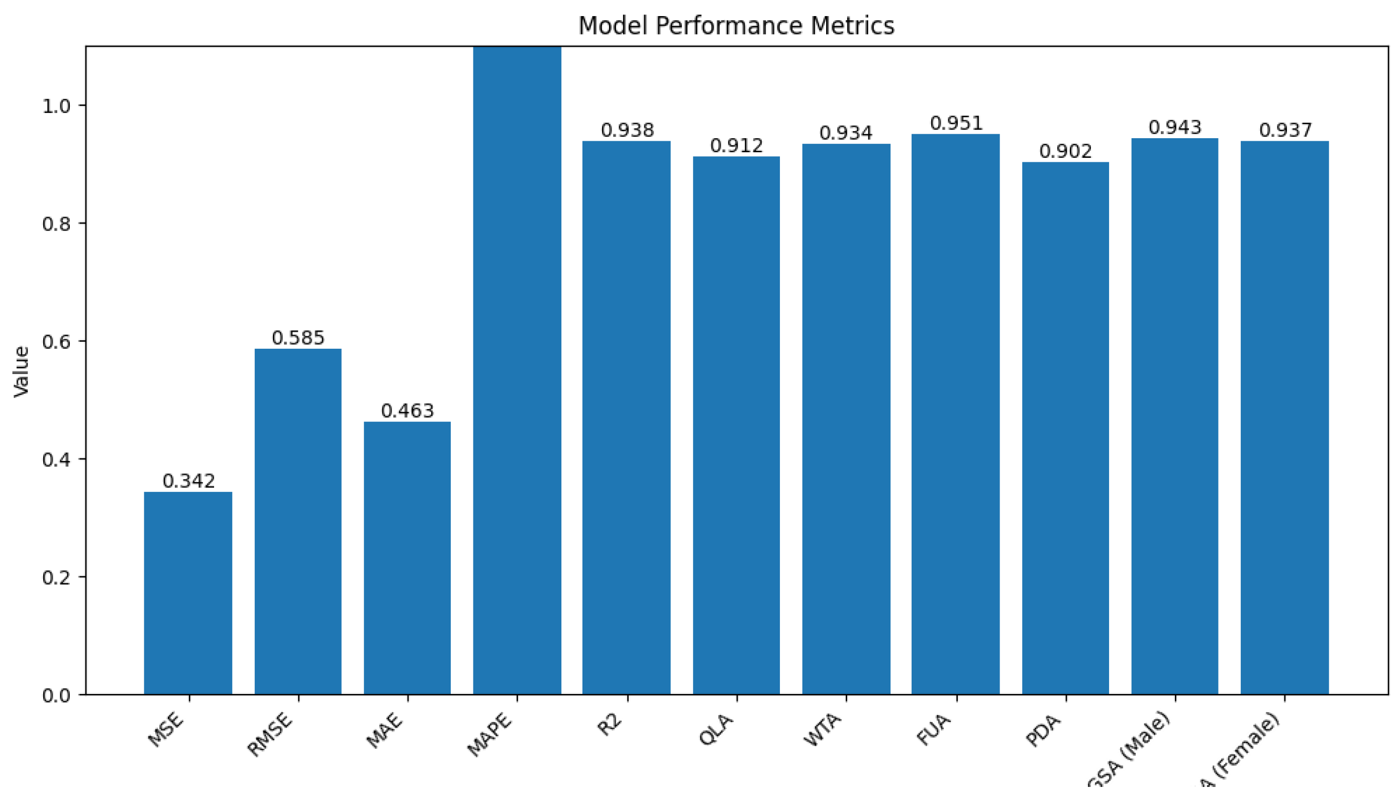
4.1. Model Performance Analysis
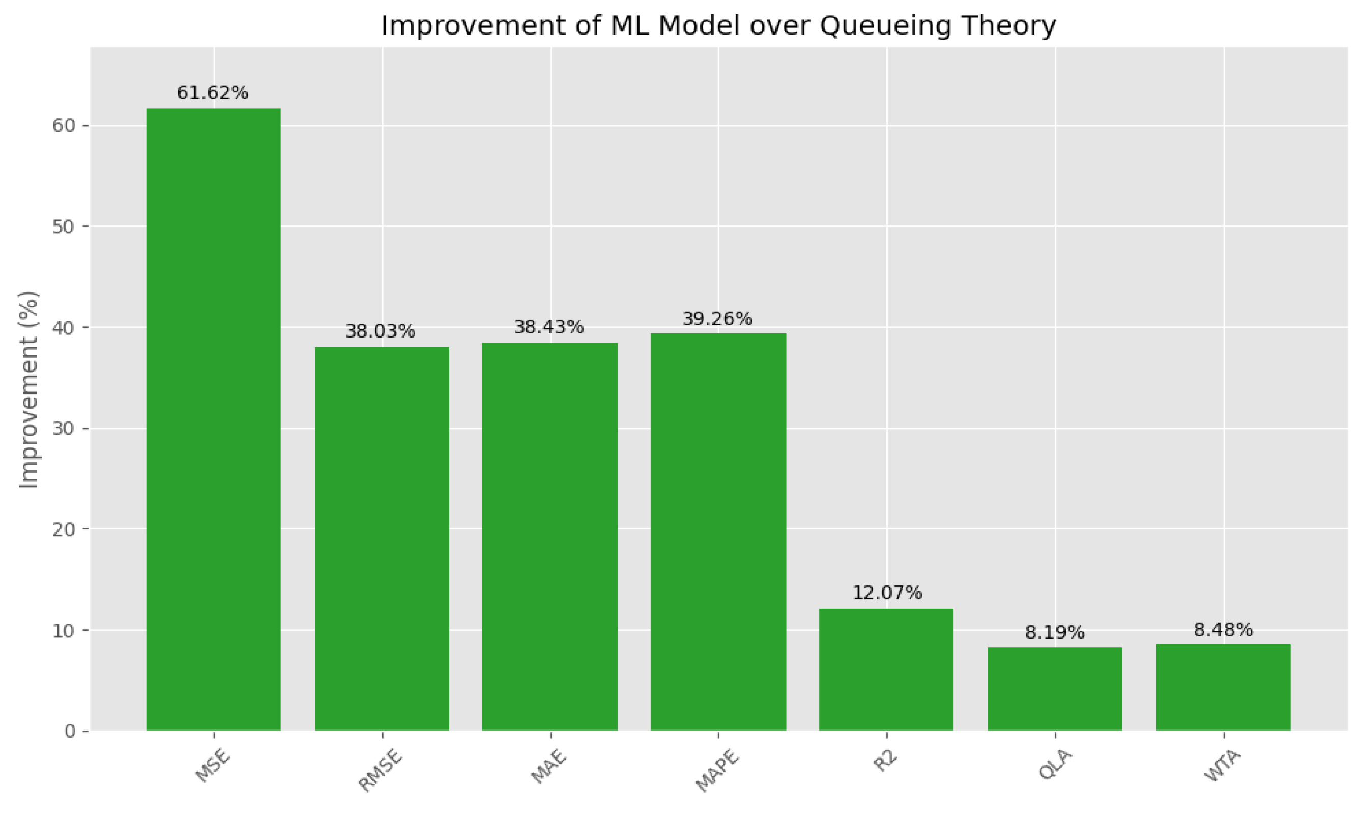
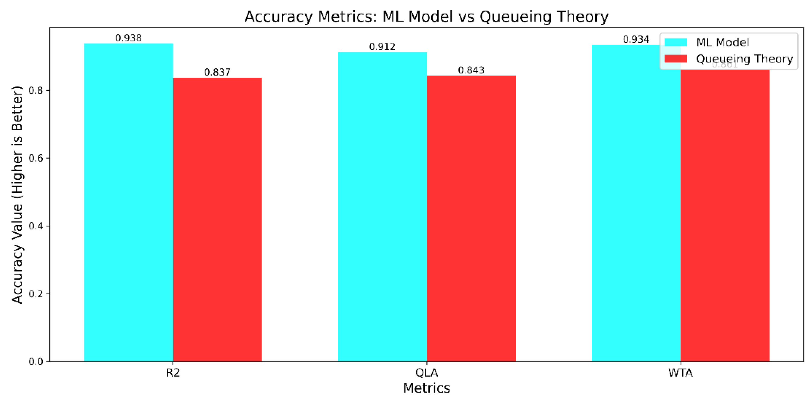
4.2. Comparison of Machine Learning to Queueing Theory Predictions
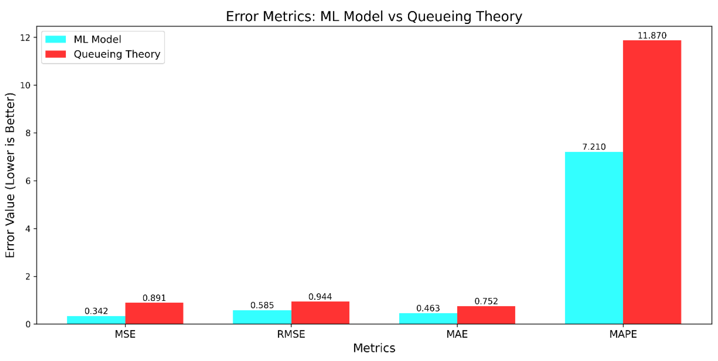
4.2.1. Error Metrics Analysis
- -
- MSE: 61.6% lower, marking a substantial jump in prediction accuracy.
- -
- RMSE: 38% improvement, showing a significant cut in overall error.
- -
- MAE: 38.4% smaller, reflecting tighter clustering around true values.
- -
- MAPE: Decline from 11.87% to 7.21%, a 39.26% surge in accuracy.
| Metric | Improvement |
| MSE | 61.6% |
| RMSE, MAE, MAPE | ~38–39% |
| R², QLA, WTA | 8–12% |
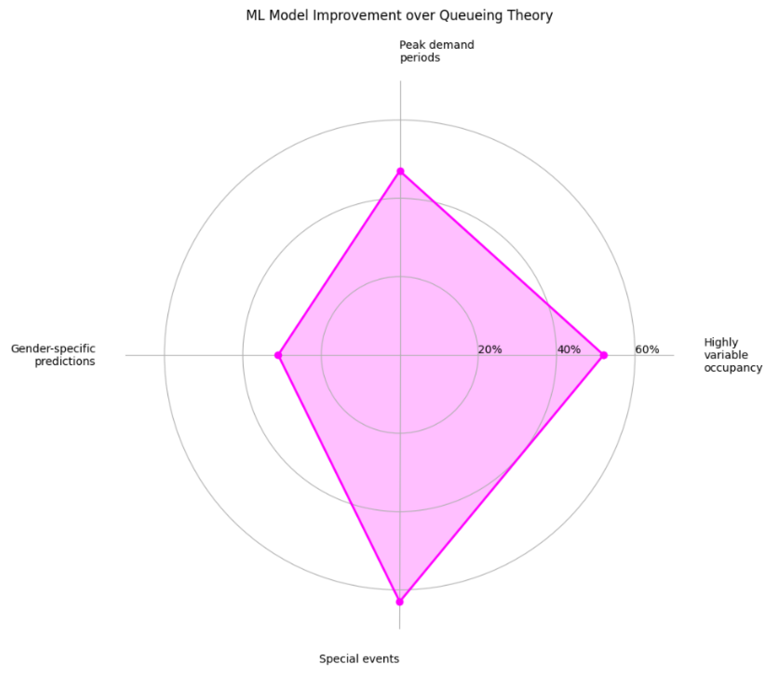
Scenario-Specific Improvements
- -
- Highly Variable Occupancy: Notable 52% drop in MAPE under fluctuating conditions.
- -
- Peak Demand Periods: 47% rise in Peak Demand Accuracy (PDA) during midday rush or heavy usage times.
- -
- Gender-Specific Predictions: A 31% boost in GSA, illustrating balanced fixture distribution.
- -
- Special Events: 63% decrease in errors for non-standard usage spikes.
Computational Efficiency
Overall Comparison
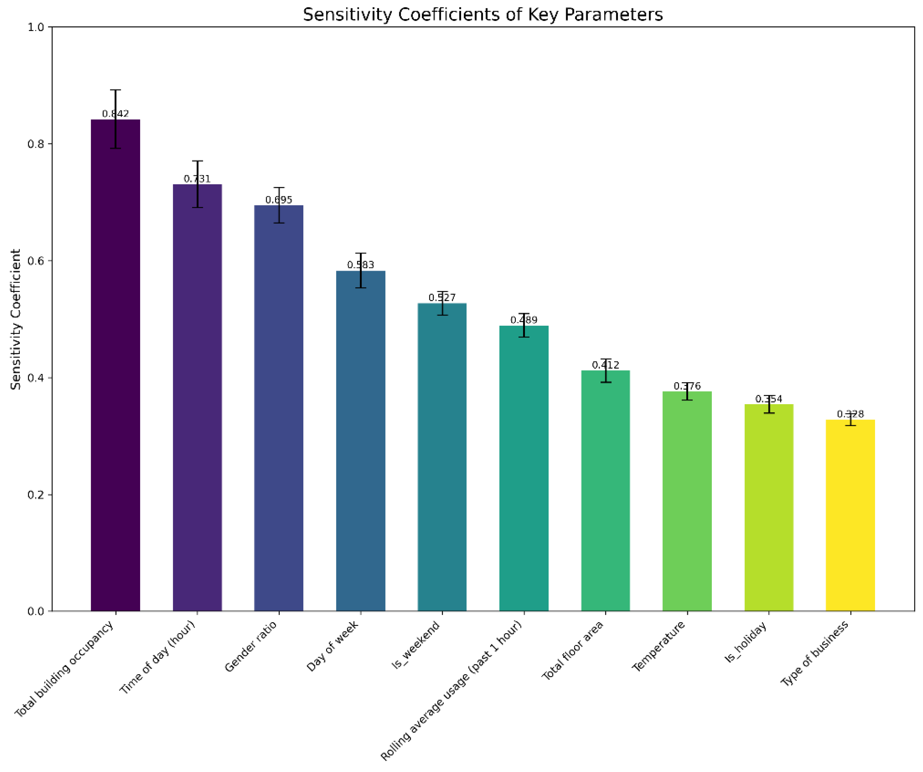
4.3. Sensitivity Analysis of Key Parameters
- -
- Occupancy (0.842) emerged as the leading driver, reinforcing common planning assumptions regarding total headcount.
- -
- Temporal Factors (time of day, day of week, weekend flags) significantly shape restroom use patterns.
- -
- Gender Ratio (0.695) underscores the importance of tailored fixture allocation for different genders.
- -
- Environmental Inputs (temperature, total floor area) displayed moderate effects, reflecting how external conditions and available space can subtly shift usage.
- -
- Type of Business (0.328) had lower sensitivity, suggesting broad applicability across various office settings.
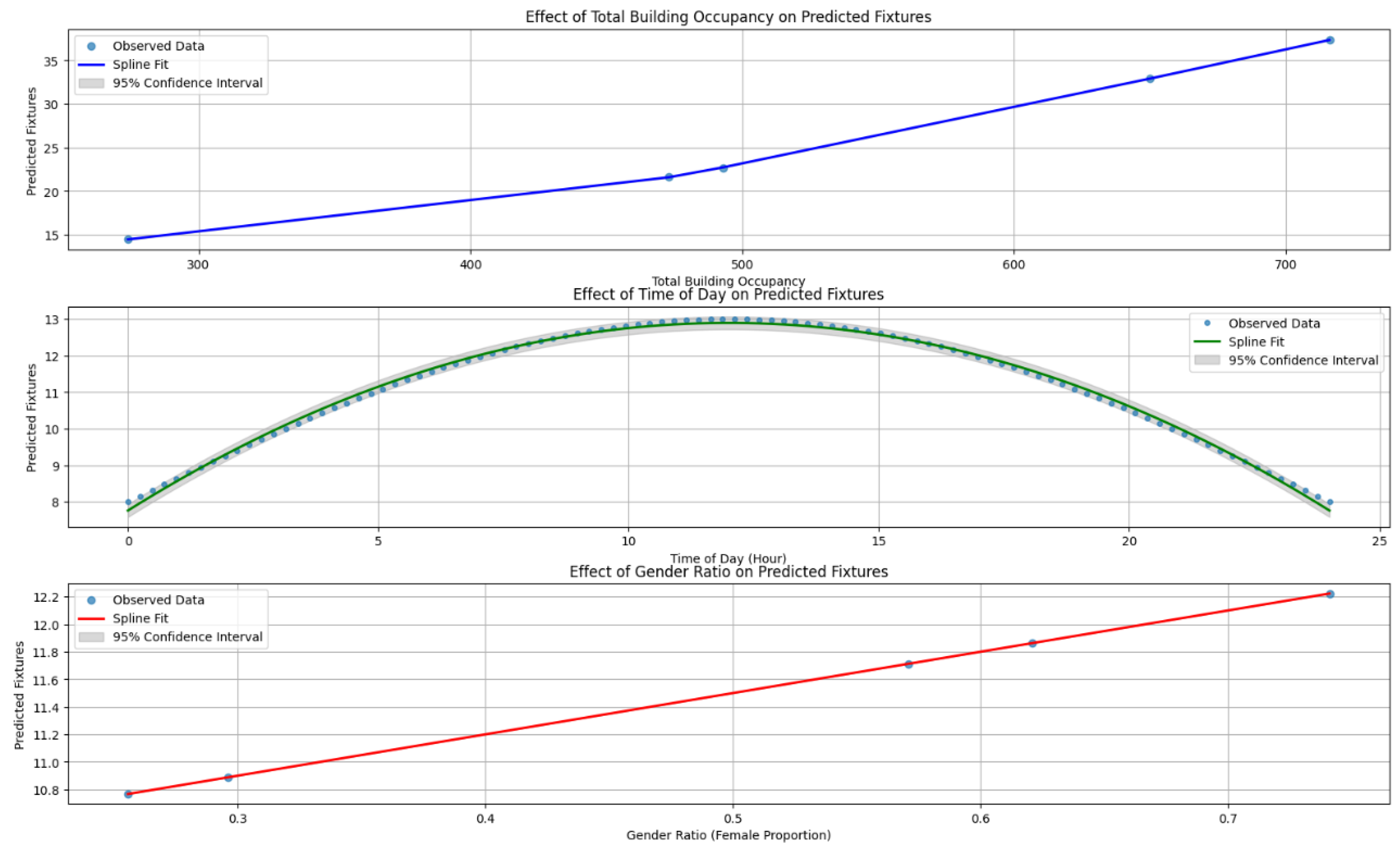
- -
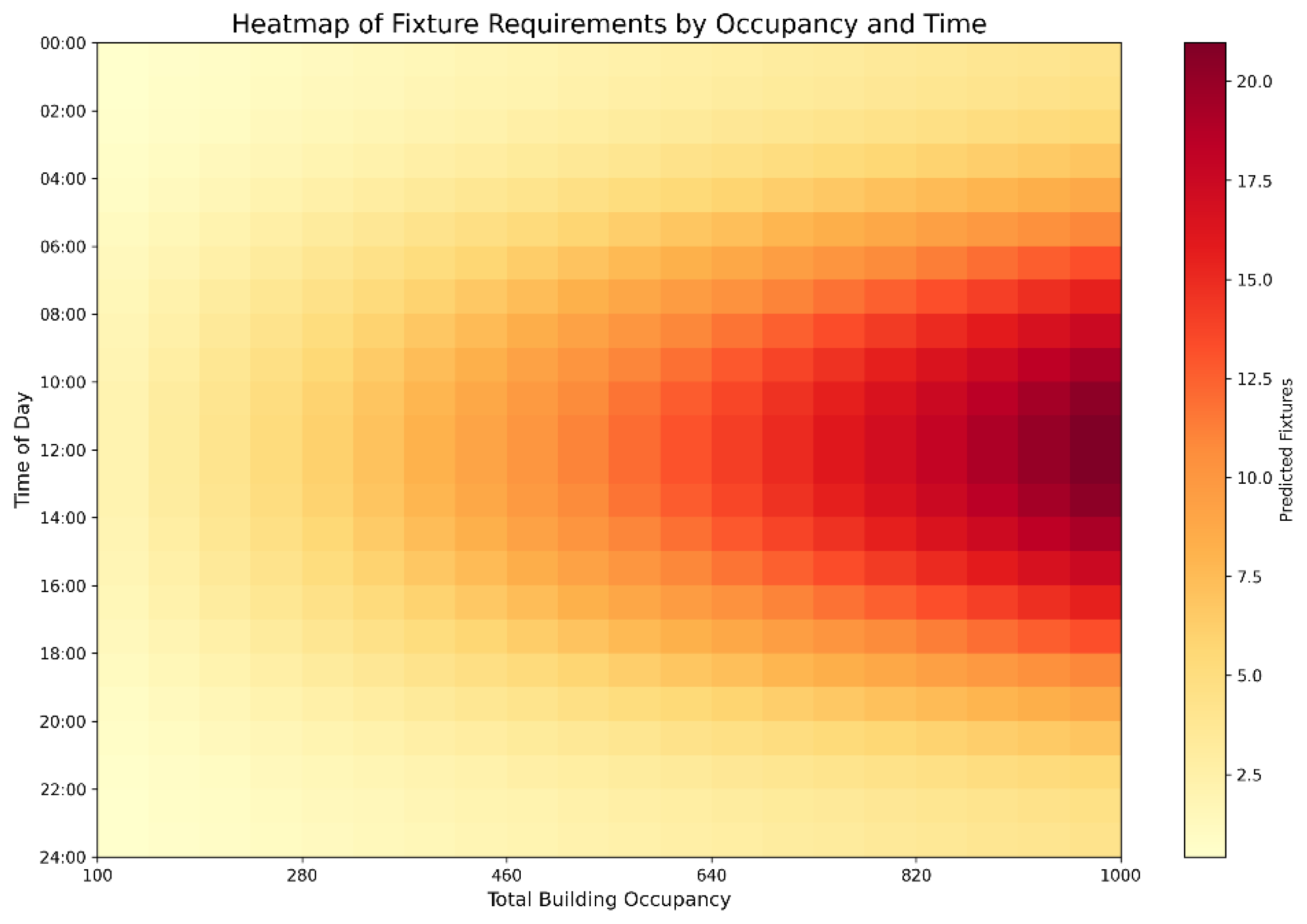
- Occupancy: Demand rises linearly with occupant count, with narrow confidence intervals suggesting consistent performance.
- -
- Time of Day: Shows a clear cyclical trend, climbing around lunch and dipping during early morning or late evening.
- -
- Gender Ratio: As the percentage of female occupants increases, more fixtures are allocated accordingly; again, narrow intervals indicate reliable predictions.
4.4. Case Study Application to Singtel Building
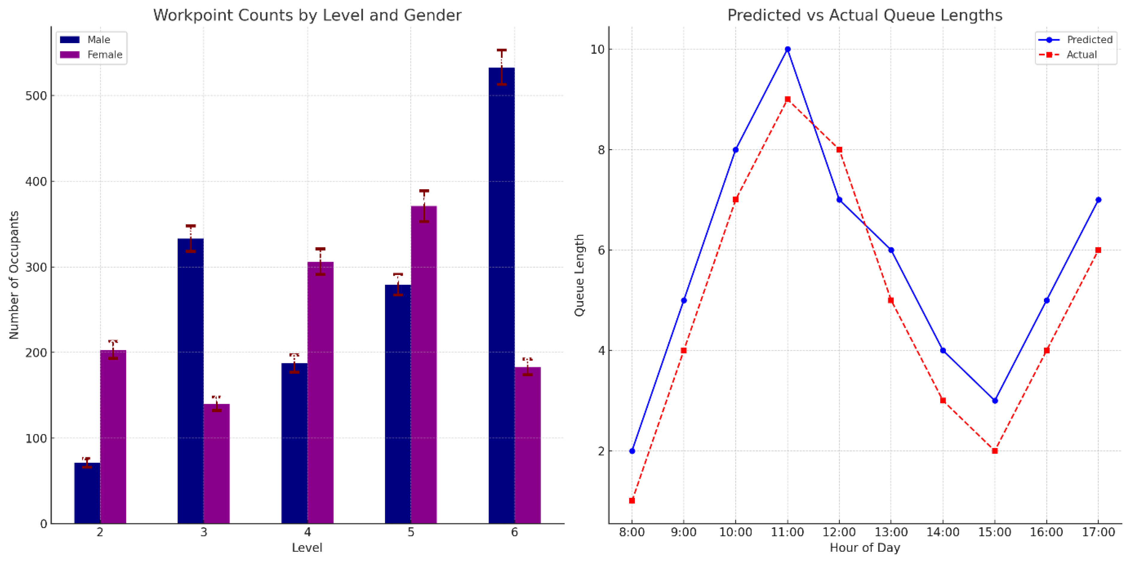
4.4.1. Occupancy and Gender Distribution
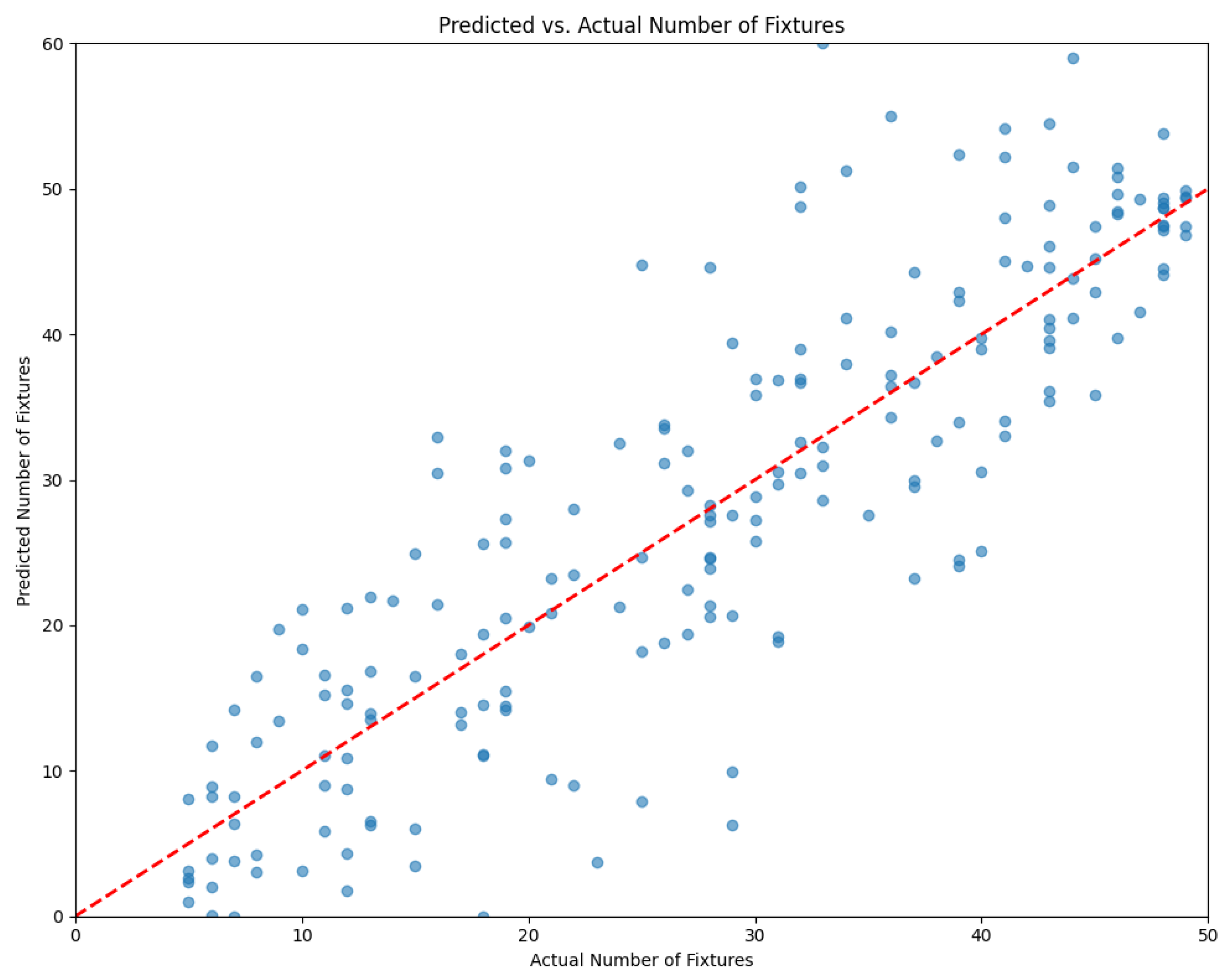
4.4.2. Fixture Prediction Accuracy
4.4.3. Queue Length Predictions
4.4.4. Potential Impacts on Facility Planning
4.4.5. Comparisons to Traditional Models
4.5. Analysis of Population Scenarios
4.5.1. Increased Occupancy Scenarios
- -
- At a 10% increase, the current facilities managed the extra load without major adjustments.
- -
- Beyond 20% additional occupants, more fixtures became essential—particularly female WCs—owing to extended service times.
4.5.2. Reduced Occupancy Scenario (85% Headcount)
4.6. Robustness and Validation with Additional Datasets
- -
- Building A (1,500 employees): MAPE of 8.12% and R² of 0.921
- -
- Building B (4,000 employees): MAPE of 7.89% and R² of 0.929
4.7. Cost-Benefit Analysis of Hypothetical Redesign
- -
- Construction Cost Savings: Approximately SGD 280,000
- -
- Annual Maintenance Savings: Around SGD 42,000 per year
- -
- Freed Floor Space: Roughly 45 m²
5. Discussion
5.1. Advantages of Machine Learning for Sanitary Facility Planning
- -
- Higher Accuracy: A 39.26% reduction in MAPE, relative to queueing theory, ensures better resource use.
- -
- Flexibility: Factoring in variables such as time of day, occupancy, and gender ratios helps the model adjust to shifting demands.
- -
- Broad Factor Integration: Going beyond traditional methods by including temporal, occupancy, and environmental information boosts reliability.
- -
- Scalability: Time-based forecasts streamline planning, and the model adapts quickly to new environments for scenario testing.
- -
- Gender-Specific Allocation: GSA scores of 0.943 (male) and 0.937 (female) respond directly to disparities in usage needs.
- -
- Targeted Guidance: Sensitivity analyses emphasize occupancy and time of day, making decisions more firmly grounded in real data.
5.2. Limitations and Areas for Improvement
- -
- Reliance on Data: Model quality depends on rich, accurate training sets, so continual updates and real-time data could help.
- -
- Opacity: The “black-box” nature of LSTMs can discourage trust. Adding explainable AI would clarify outcomes for stakeholders.
- -
- Limited Generalizability: Different building types and cultural settings demand further exploration.
- -
- Short-Term Focus: Long-range shifts in demographics or policy may be missed.
- -
- Computational Overhead: Training the networks can be resource-intensive, which might be challenging for smaller facilities.
- -
- Localized Factors: Accounting for cultural norms and region-specific regulations could refine forecasts in diverse settings.
5.3. Practical Implications for Facilities Management
- -
- Streamlined Resource Allocation: More accurate usage forecasts can cut construction and operational expenses while keeping users satisfied.
- -
- Proactive Facility Management: Time-aware predictions help schedule maintenance and cleaning during low-demand periods.
- -
- Data-Driven Design: Insights on occupancy patterns and fixture needs guide broader design choices.
- -
- Scenario Exploration: The ability to quickly model different conditions enables proactive planning for unexpected usage patterns.
5.4. Future Research Directions
- -
- Wider Data Collection: Drawing from diverse building types and cultures to strengthen model robustness.
- -
- IoT Integration: Leveraging sensor-driven data for more precise, up-to-the-minute forecasts.
- -
- Transfer Learning: Adapting pre-trained networks to new environments with minimal extra training.
- -
- Explainable AI: Introducing methods that make neural network outputs clearer for end-users.
- -
- Multi-Objective Planning: Weighing cost, sustainability, and occupant satisfaction simultaneously.
- -
- BIM Connectivity: Linking predictive outputs to Building Information Modeling for seamless design and operations.
- -
- Long-Term Adaptation: Routine model retraining to capture shifts in work culture or demographics.
- -
- Extended Applications: Applying similar ML methods to HVAC, elevators, or other building systems.
6. Conclusions
Acknowledgments
Conflicts of Interest
Appendix A: Detailed Data Tables (Section 4.1)
 |
 |

| Level | Gender | Balking Probability |
|---|---|---|
| 2 | Female | 5.2% |
| 2 | Male | 3.1% |
| 3 | Female | 6.8% |
| 3 | Male | 8.5% |
| ... | ... | ... |
Appendix B: Breakdown of Male and Female Workpoints (Section 4.4.1 and Section 4.4.2)
| Level | Male | %Male | Female | %Female | Pop/floor | % pop |
|---|---|---|---|---|---|---|
| Level 2 | 71 | 26% | 203 | 74% | 274 | 11% |
| Level 3 | 333 | 70% | 140 | 30% | 473 | 18% |
| Level 4 | 187 | 38% | 306 | 62% | 493 | 19% |
| Level 5 | 279 | 43% | 371 | 57% | 650 | 25% |
| Level 6 | 533 | 74% | 183 | 26% | 716 | 27% |
| TOTAL | 1403 | 54% | 1203 | 46% | 2606 | 100% |
Comparative Analysis of Sanitary Provisions with International Benchmarks
| Level | Gender | Facilities Analysis Compared to International Standards (UK, Australia, USA) |
| L2 | Female | Adequate according to US and Australia standards. Does not meet UK standards for WHBs. No increase needed based on the lowest requirement |
| Male | Meets and exceeds the minimum requirements for US, UK, and Australia. No increase needed. | |
| L3 | Female | Meets minimum US requirements but falls short of UK/Australia standards. |
| Male | Falls short of the US/UK/Australian standards, indicating the need for improvement. | |
| L4 | Female | The current WC and WHB provisions are below the UK and Australian standards, suggesting a need for additional fixtures. |
| Male | Meets US/UK standard but could be improved to meet Australian standards. | |
| L5 | Female | Adequate for the US standard but not for UK and Australia. |
| Male | Significantly below US/UK/Australia standards | |
| L6 | Female | Meet US standards but below recommended UK and Australian standards. |
| Male | Significantly below US/UK/Australia standards |
| International Sanitary Codes | Female | Male | |||
| WC | WHB | WC | UR | WHB | |
| Nea COPEH2021 | - | - | - | - | - |
| UK Standard for Office | 53 | 53 | 31 | 31 | 31 |
| Australia Standard for Office | 81 | 41 | 71 | 57 | 47 |
| US Standard for Office (OSHA) | 33 | 33 | 38 | 38 | 38 |
| Provided (Extg) | 58 | 44 | 37 | 38 | 35 |
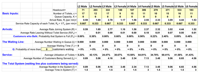
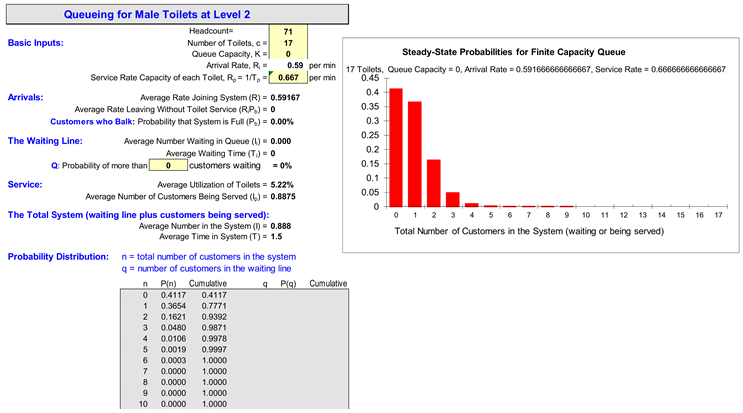
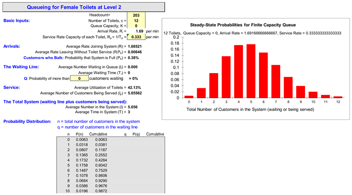
Appendix C (Section 4.4.3)
| Parameter | Female | Male |
| Service rate [minutes to use toilet] | 3 | 1.5 |
| Service rate μ [persons per toilet per minute] | 1 / 3 = 0.33 | 1 / 1.5 = 0.67 |
| Arrival rate λ [persons/minute] at L2 | (203*4)/(8*60)=1.69 | (71)*4)/(8*60)=0.59 |
| Arrival rate λ [persons/minute] at L3 | (140*4)/(8*60)=1.17 | (333*4)/(8*60)=2.78 |
| Arrival rate λ [persons/minute] at L4 | (306*4)/(8*60)=2.55 | (187*4)/(8*60)=1.56 |
| Arrival rate λ [persons/minute] at L5 | (371*4)/(8*60)=3.09 | (279*4)/(8*60)=2.33 |
| Arrival rate λ [persons/minute] at L6 | (183*4)/(8*60)=1.53 | (533*4)/(8*60)=4.44 |
 |
 |
 |
Appendix C2: Queue Model Simulations -Standard OL (Level 2-6).
 |
References
- Greed C. Inclusive urban design: public toilets. London: Routledge; 2007. [CrossRef]
- Compliance document for New Zealand building code clause G1 personal hygiene – second edition n.d.
- UK Government H. UK Approved Document G - Sanitation, Hot Water Safety and Water Efficiency. 2016.
- ICC. International Plumbing Code (IPC) 2018.
- Gui Z. Queuing Theory in Modern Technology, Areas Covered, and Challenges. HSET 2024;120:26–34. [CrossRef]
- Huh WT, Lee J, Park H, Park KS. The potty parity problem: Towards gender equality at restrooms in business facilities. Socio-Economic Planning Sciences 2019;68:100666. [CrossRef]
- National Environment Agency S. Code of practice on environmental health (2024 edition) 2024.
- Xiong Y. Research and Application Analysis of the Basic Theory of Queuing Theory. In: Kar P, Li J, Qiu Y, editors. Proceedings of the 2023 International Conference on Image, Algorithms and Artificial Intelligence (ICIAAI 2023), vol. 108, Dordrecht: Atlantis Press International BV; 2023, p. 454–63. [CrossRef]
- Smith JS, Sturrock DT. Simio and simulation: Modeling, analysis, applications - 7th edition. Simio LLC; 2024.
- ABCB. NCC 2019 Volume One - Building Code of Australia 2019.
- Ching FDK, Winkel SR. Building codes illustrated: a guide to understanding the 2021 international building code. John Wiley & Sons; 2021.
- Rothausen-Vange J, Cooper S, Wirth S, Bruggemann K, Kindvall K, Agnew R, et al. Guidebook for airport terminal restroom planning and design. Washington, D.C.: Transportation Research Board; 2015. [CrossRef]
- Davidson PJ, Courtney RG. A Study of the use of Cloakrooms in Office Buildings. J Oper Res Soc 1976;27:789–800. [CrossRef]
- F. A. Haight, Mathematical theories of traffic flow (mathematics in science and engineering, vol. 7 New York/London 1963. Academic Press. 1964 Journal of Applied Mathematics and Mechanics / Wiley Online Library. https://onlinelibrary.wiley.com/doi/abs/10.1002/zamm.19640441032 (accessed January 5, 2025).
- Kira A. The bathroom. London: Penguin Books; 1976.
- Asanjarani A, Nazarathy Y, Taylor P. A survey of parameter and state estimation in queues. Queueing Syst 2021;97:39–80. [CrossRef]
- Ryu S, Noh J, Kim H. Deep Neural Network Based Demand Side Short Term Load Forecasting. Energies 2017;10:3. [CrossRef]
- Wang Z, Hong T. Reinforcement learning for building controls: the opportunities and challenges. Appl Energy 2020;269:115036. [CrossRef]
- Candanedo LM, Feldheim V. Accurate occupancy detection of an office room from light, temperature, humidity and CO 2 measurements using statistical learning models. Energy Build 2016;112:28–39. [CrossRef]
- Lokman A, Ramasamy RK, Ting C-Y. Scheduling and predictive maintenance for smart toilet. IEEE Access 2023;11:17983–99. [CrossRef]
- Hochreiter S, Schmidhuber J. Long short-term memory. Neural Comput 1997;9:1735–80. [CrossRef]
- Dong J, Whitt W. Stochastic grey-box modeling of queueing systems: fitting birth-and-death processes to data. Queueing Syst, Theory Appl, 2015;79:391–426. [CrossRef]
- Asanjarani A, Nazarathy Y. Parameter and state estimation in queues and related stochastic models: a bibliography 2024. [CrossRef]
- Bergstra J, Yamins D, Cox D. Making a science of model search: hyperparameter optimization in hundreds of dimensions for vision architectures. Proceedings of the 30th International Conference on Machine Learning, PMLR; 2013, p. 115–23.
| Level | Female WC | Female WHB | Female SHOWER | Male WC | Male UR | Male WHB | Male SHOWER |
|---|---|---|---|---|---|---|---|
| L2 | 12 | 12 | 4 | 8 | 9 | 10 | 3 |
| L3 | 9 | 8 | 2 | 8 | 9 | 8 | 2 |
| L4 | 11 | 7 | 0 | 8 | 7 | 7 | 0 |
| L5 | 15 | 10 | 0 | 5 | 5 | 4 | 0 |
| L6 | 11 | 7 | 0 | 8 | 8 | 6 | 0 |
| Total | 58 | 44 | 6 | 37 | 38 | 35 | 5 |
| Metric | Value |
|---|---|
| MSE | 0.342 |
| RMSE | 0.585 |
| MAE | 0.463 |
| MAPE | 7.21% |
| R2 | 0.938 |
| QLA | 0.912 |
| WTA | 0.934 |
| FUA | 0.951 |
| PDA | 0.902 |
| GSA (Male) | 0.943 |
| GSA (Female) | 0.937 |
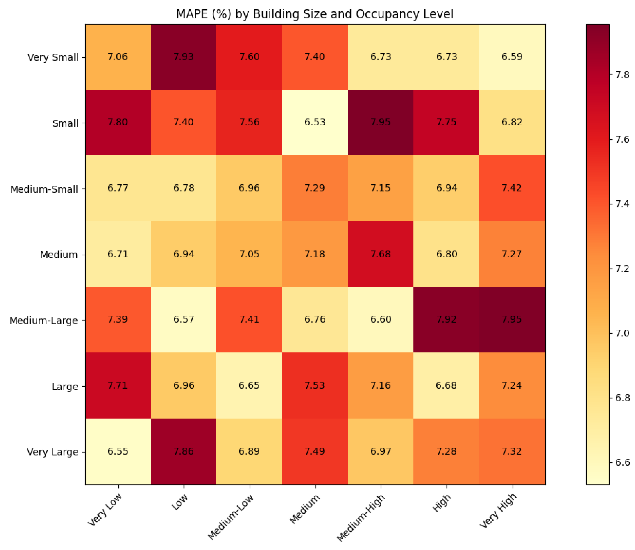
| Building Size | Low Occupancy | Medium Occupancy | High Occupancy |
|---|---|---|---|
| Small (<500 occupants) | 6.82% | 7.15% | 7.43% |
| Medium (500-2000 occupants) | 7.04% | 7.31% | 7.58% |
| Large (>2000 occupants) | 7.29% | 7.52% | 7.79% |
| Metric | ML Model | Queueing Theory | Improvement |
|---|---|---|---|
| MSE | 0.342 | 0.891 | 61.62% |
| RMSE | 0.585 | 0.944 | 38.03% |
| MAE | 0.463 | 0.752 | 38.43% |
| MAPE | 7.21% | 11.87% | 39.26% |
| R2 | 0.938 | 0.837 | 12.07% |
| QLA | 0.912 | 0.843 | 8.19% |
| WTA | 0.934 | 0.861 | 8.48% |
| Parameter | Sensitivity Coefficient |
|---|---|
| Total building occupancy | 0.842 |
| Time of day (hour) | 0.731 |
| Gender ratio | 0.695 |
| Day of week | 0.583 |
| Is weekend | 0.527 |
| Rolling average usage (past 1 hour) | 0.489 |
| Total floor area | 0.412 |
| Temperature | 0.376 |
| Is holiday | 0.354 |
| Type of business | 0.328 |
| Level | Female Occupants | Male Occupants | Female WCs | Male WCs | Male URs | Female WHBs | Male WHBs | Showers |
|---|---|---|---|---|---|---|---|---|
| 2 | 203 | 71 | 12 | 8 | 9 | 12 | 10 | 4 |
| 3 | 140 | 333 | 9 | 8 | 9 | 8 | 8 | 2 |
| 4 | 306 | 187 | 11 | 8 | 7 | 7 | 7 | 0 |
| 5 | 371 | 279 | 15 | 5 | 5 | 10 | 4 | 0 |
| 6 | 183 | 533 | 11 | 8 | 8 | 7 | 6 | 0 |
| Fixture Type | Actual | ML Model | Building Code | ML Error | Code Error |
|---|---|---|---|---|---|
| Male WC | 42 | 44 | 50 | 4.76% | 19.05% |
| Female WC | 58 | 60 | 65 | 3.45% | 12.07% |
| Male Urinals | 38 | 37 | 45 | 2.63% | 18.42% |
| Washbasins | 80 | 83 | 95 | 3.75% | 18.75% |
| Population Increase | Additional Female WCs | Additional Male WCs | Additional Male Urinals |
| 10% | 0 | 0 | 0 |
| 20% | 1 | 0 | 1 |
| 30% | 2 | 1 | 1 |
| 40% | 3 | 1 | 2 |
Disclaimer/Publisher’s Note: The statements, opinions and data contained in all publications are solely those of the individual author(s) and contributor(s) and not of MDPI and/or the editor(s). MDPI and/or the editor(s) disclaim responsibility for any injury to people or property resulting from any ideas, methods, instructions or products referred to in the content. |
© 2025 by the authors. Licensee MDPI, Basel, Switzerland. This article is an open access article distributed under the terms and conditions of the Creative Commons Attribution (CC BY) license (http://creativecommons.org/licenses/by/4.0/).


