
Submitted:
03 January 2025
Posted:
06 January 2025
You are already at the latest version
Abstract
The well-regarded feedforward control strategy known as Input Shaping is aimed at improving the dynamic response of flexible mechanical systems by reducing overshoot and residual vibration amplitude. Its validity has been confirmed by numerous studies dealing with linear system dynamics. However, its application to nonlinear systems, particularly those influenced by tractive-elastic rolling contact friction, remains a challenging and less explored open research area. This paper investigates whether Input Shaping, without tractive rolling friction compensation, can effectively mitigate vibrations in a trolley-pipe benchmark transport system. In this system, the pipe is modeled as a rolling disk attached to the trolley by a spring at its center of mass, while the trolley itself is connected to a guiding body frame by an additional spring acting as a proportional control. The natural frequencies of the system are analytically estimated and numerically verified from a corresponding well suited multibody model. Thus tailored two-mode shapers are designed based on simultaneous constraints and convolution sum respectively. Through multibody simulations, this study evaluates the performance of Input Shaping under tractive-elastic rolling contact friction conditions. The findings highlight both the potential and limitations of this control method in addressing nonlinear mechanical systems influenced by such tractive-elastic rolling contact friction.
Keywords:
Input Shaping
; Tractive-Elastic
; Rolling Contact Friction
; Multibody Dynamics
; Nonlinear Systems
; Flexible Systems
; Dynamic friction Compensation
1. Introduction
1.1. Motivation
Input Shaping is a feedforward control technique designed to reduce or eliminate residual vibrations in flexible mechanical systems. Its origins can be traced back to the Posicast Control developed by O. J. Smith in 1957, which laid the groundwork for addressing transient oscillations in dynamic systems [1]. In the early 1990s, Neil Singer and Warren Seering further developed this idea, refining it into what is now widely recognized as Input Shaping [2]. Since then, William Singhose, a Ph.D. student of Seering, has become one of the most prolific contributors to this field, publishing extensively on its applications and methodologies [3].
Over the years, Input Shaping has proven to be a versatile and robust control strategy, with successful implementations in a wide range of applications. These include experimental studies conducted during the NASA Shuttle Program [4] as well as practical applications in overhead cranes, flexible manipulators, and linear mechanical systems in Transportation Engineering [5].
The process of shaping an input command involves convolving the original command with the selected input shaper. Typical input shapers include the Zero Vibration (ZV) shaper and the Zero Vibration and Derivative (ZVD) shaper. The ZV shaper, comprising only two coefficients, ensures that the residual vibration caused by a sequence of autocanceling impulses is entirely eliminated. In contrast, the ZVD shaper, by including additional constraints, not only nullifies the residual vibration but also its first derivative, providing enhanced robustness to modeling inaccuracies and frequency estimation errors.
Figure 1 demonstrates this operation using a ZV filter applied to a step input command. The velocity command before and after shaping is shown, along with the corresponding payload response. The shaped command smooths out abrupt transitions, redistributing the input energy to mitigate vibratory effects. As a result, the residual vibration in the payload response is significantly reduced, underscoring the effectiveness of the ZV shaper.
Despite its effectiveness in linear systems, extending Input Shaping to nonlinear systems presents significant challenges. Heckman and J. Lawrence, students of Singhose, made early attempts to apply Input Shaping to systems with Coulomb friction under gross sliding conditions. Their work used compensators to linearize the system, achieving moderate success [6] However, the application of Input Shaping to systems with tractive-elastic rolling contact friction is far more complex due to the nonlinearity introduced by the directional dependency of such friction force on multibody system accelerations.
This study builds on the foundational work in the field and investigates the application of Input Shaping to nonlinear systems characterized by tractive-elastic rolling contact friction. The unique challenges posed by this friction resistance type highlight the need for innovative approaches to extend the benefits of Input Shaping beyond linear scenarios.
Is the propose of this primary study on the subject to describe how tractive-elastic rolling contact frictional effects in flexible systems affect to Input Shaping performances and how overcome them.
1.2. Background: Previous Works
Command generation techniques that reduce vibration and compensate for gross sliding friction have been investigated in [7]. The provided Figure 2 illustrates two representations of a mass-spring-damper nonlinear system undergoing gross-sliding friction, where subfigure (a) depicts the benchmark mechanical physical representation composed of a mass m which moves horizontally, a spring with stiffness that applies a restoring force proportional to the displacement x a damping element with coefficient which resist motion proportional to velocity, lumped together become a PD-control for the system displacement x as a result of the Input Motion r feed by an external command generator. Note that the mass displacement is influenced by non-linear gross-sliding friction , where is the magnitude of the friction force and denotes its direction. The system models real-world dynamics where frictional forces cause resistance in motion by gross-sliding, modeled by the kinetic friction coefficient . Dealing with subfigure (b) ie. the block diagram representation, this provides a mathematical equivalent of the physical system: the input signal r represents the desired position, the signal is compared to the current position x to generate the error. A block containing the spring and damping characteristics of a PD-control process the error.The nonlinear gross-sliding friction block adds a force opposing the motion, making the system non-linear. The plant block represents the dynamics of the mass, where acceleration integrates to velocity and position. The flow of signals through the blocks models the interaction of forces and the term introduces nonlinearity, making the system behaviour more complex compared to the purely linear mass-spring-damper system, and given by
Many texts [8,9] provide an analytical solution for the system represented in Figure 2. Without including the derivative action of the damper, that is, if the only damping considered is the one caused by Coulomb friction in gross-slip, then the decrease in the vibration amplitude is not logarithmic -as in the case of viscous damping proportional to velocity- but linear, depicted in Figure 3. In the literature [8,9], it is demonstrated that its value is given by:
Where , is the coefficient of kinetic friction, are the vibration amplitude at n+1 and n sampling times respectively being . Shortly, to briefly clarify how the non-linear gross slip friction term affects system behavior the Figure 3 shows the response to one unit not null initial position condition.
Figure 3 also shows that Coulomb friction causes the existence of multiple equilibrium positions, which indeed occur. The equilibrium positions can be determined by enforcing static equilibrium in the x-direction. The solution is a region defined by:
Depending on the initial conditions, the response will settle at a value somewhere within this equilibrium region. Moreover, if the mass is subjected to an initial displacement within this equilibrium region, it will remain stationary as long as the initial velocity is zero. Shortly Equation 3 reveals that increasing the proportional gain of the system will decrease the final error.
1.3. Rolling Friction: brief review
Effects of Rolling friction have been described in detail by Johnson (1985) [10] and only the more salient points will be considered here. From a kinematics view point Rollling is the relative angular velocity between the two bodies about an axis lying in the tangent plane. Following Jhonson (1985) we define free rolling as a rolling motion in which the tangential force f is cero, and tractive rolling as rolling motion in which the tangential force f is non-zero but less than the limiting value :
at which gross sliding occurs, and the direction of f is directly opposed to the direction of such gross sliding. Regarding the tractive rolling case, actually the interfacial forces lead to a contact area of finite size shown in Figure 4, thus the distribution of forces over this area can, therefore, lead to the transmission of a moment across the interface.
In mechanical rolling contact situations, there is resistance to rolling, although its magnitude becomes much smaller than the resistance to sliding.Thus, considering an elastic rolling contact between the cylinder freely rolling on the trolley of our reference model under a normal load P per unit length in the axial direction of the cylinder, as illustrated in the Figure 4, the local pressure, p, in the contact zone, and the contact semiwidth, a, are known form the Hertz equations [11,12].
Considering the striped strip in the Figure 4 of width dx at point x, we can see that, during forward compression of the contacting material, the normal force per unit length of the roller will be p·dx, and this will exert a resistive moment about the centre of the contact zone whose magnitude is px dx. Thus, the total moment exerted by all the elements on the front half of the roller cylinder will be
If the cylinder rolls forward through a distance x, the elastic work done by this couple is given by
Under ideal conditions the cylinder would be subjected to an equal and opposite moment arising from the pressure distribution in the rear half of the contact. However, owing to elastic hysteresis losses, not all the work is recovered and there is some dissipation energy. If we define the hysteresis loss by a coefficient , thus the energy dissipated in rolling a distance x will be and if this loss represents the rolling resistance, it follows that
Where F is the force required to overcome the resistance. By analogy with sliding friction, the ratio can be defined as the coefficient of rolling resistance, , where
Nonetheless, it is important to differentiate between losses in elastic contacts as the just studied case and losses in the presence of plastic deformations. Thus, rolling resistance in other cases arises from deformation-related losses. When considering deformation-related losses in a primary analysis, subsurface plastic deformation occurs only when the contact pressure on first contact exceeds a certain threshold value. If this is the case, the energy dissipated in such deformation can be considerably higher than that of the aforementioned due to elastic hysteresis. However, owing to the accumulation of stress cycles during rolling, the degree of plastic deformation reduces with cycling, thus after a relative number of cycles, the deformation becomes fully elastic. This process is referred to as [13]. For this reason, this work assumes that load do not exceeds the limit stress and thus the present study limits to the free rolling of an elastic cylinder on a elastic-perfectly contact. Regarding the overall Figure 5, it reinforces the notion that under the elastic contact conditions, the response of the Trolley-Cylinder system remains undamped, provided that hysteresis losses are considered negligibly small. Figure 5b depicts the impulse response of the roller, highlighting the nearly undamped x-position of its mass center. The response was obtained using Simscape Multibody Matlab Toolbox to numerically integrate the equations of motion for this benchmark mechanical system.
2. Materials and Methods
In any customary Input Shaping problem, the first step in addressing the design of an Input Shaping filter is to develop a simplified plus affordable model of the system that allows for the estimation of its natural frequencies. In the actual system model, the pipe is modeled as a rolling disk attached to the trolley by a spring at its center of mass, while the trolley itself is connected to a guiding body frame by an additional spring acting as a proportional control. In this work, modelling is divided into a single model based on Free Body Diagrams (FBDs) plus the Newton-Euler equations and a model based on multibody analysis techniques using the Simscape Multibody Toolbox available in Matlab-Mathworks aforementioned. The natural frequencies values extracted from both models match as demonstrates the following.
2.1. Newton-Euler Equations of Motion for the Trolley-Pipe Transport System.
With reference to Figure 6 the forces acting on the two bodies consist of the spring forces plus the friction force between the disk and the cart required to overcome the rolling resistance. Also negligible small friction between the cart and the frame of reference has been assumed.
The net force on the cart, equal to its mass times acceleration, is given by the equation
Developing this equation gives
The net force on the rolling disk (pipe) is given by Equation (10) in words, the net force on the disk is equal to its mass times the acceleration of its centre of mass as follows
where f represents the rolling friction force, and denote the positions of the trolley and disk, respectively. At this point, considering the negative sign of torque due to this friction force f, the torque equation becomes:
Also from the kinematics
by substituting in equation (11) gives:
Now, substituting f into the car’s equations of motion (9) and simplifying them, we get:
Finally, dealing with the rolling disk that models the pipe:
2.2. State Matrix, and Natural Frequencies
By rewriting equations (14) and (15) in matrix form gives:
At this point switching to modal coordinates to find the natural frequencies, we solve the problem of eigenvalues and eigenvectors:
that provides
By carrying out this determinant we reach
A little algebra brings us to the quadratic equation in :
As customary, making the change of variable = , thus equation (20) can be rewriten as
Solving for
Thus, the system natural frequencies are
Using these analytical expressions of natural frequencies and values of the parameters m=1 [Kg], =k= 1[N/m], the numerical values explained in Table 1 are obtained.
2.3. The Multibody Model
To verify that the above dynamic analysis and the values corresponding to these natural frequencies are correct, a systematic treatment of the dynamic behavior of the interconnected bodies has led to a multibody model of the system set up, by means of a prismatic or translational kinematic joint between the carriage and the reference frame, treating the rolling contact between the pipe and the trolley, and a 6 DOF joint was chosen from Matlab’s Simscape-Multibody kinematic joint library. The two springs were also placed between the frame and the rear face of the trolley and the front face of the trolley with the center of mass of the pipe, although the established elastic forces are not visible in the Matlab Simscape Mechanical Explorer shown in Figure 7. The rolling contact between the pipe and the trolley was modeled using a smooth spring-damper approach, with stiffness and damping parameters detailed in Table 2 and Table 3. This approach ensures numerical stability while capturing the essential dynamics of rolling friction.
Given the inherent complexity of rolling the pipe on the trolley, the multibody model shown in Figure 8 has not been imported from any CAD before, on the contrary, it has been built by customizing the objects corresponding to the bodies, the kinematic joints and the frames transforms that have been imported directly from the Simscape Multibody toolbox plus a manual interconnection between them. About the inertial properties of bodies, the trolley has been modeled as a concentrated mass point at is mass center, in words, a newton model, while the pipe has distributed mass with not null moments of inertia plus products of inertia.
A small initial impact of the tube on the surface of the trolley causes the mechanical vibration of this flexible system. Then logging the signal corresponding to the abscissa position of the center of mass of the pipe allows experimentally measuring the system natural frequencies by carrying out the FFT of this signal. As demonstrates Figure 9 the low frequency component of the logged signal value is while the high frequency component values is . Both values, extracted from the multibody model simulation, coincides with the analytical values depicted in Table 1. This reinforces the notion that both the flexible system dynamic analysis plus the system’s multibody model are correct. Note that
2.4. Convolved ZVD-ZVD Shaper
Note that the ratio between the two natural frequencies of this two mode undamped system becomes . Input Shaping filters for undamped systems, as in this case, have the property of cancelling vibration at the modelled frequency and at odd multiples of it. Given this frequency ratio, in this case this property is not useful to us and the most appealing solution consists of using a convolved shaper resulting from the convolution sum between two ZVD filters for each of the single-mode frequency as follows
At this point by carrying out the convolution sum between these two ZVD shaper, a time delay filter (TDF) is obtained that attenuates the amplitude of the vibration at both frequencies given by
The convolved two-mode ZVD-ZVD shaper was designed to address the natural frequencies and , as defined in Equations (23). By combining two ZVD filters, this shaper attenuates vibrations at both frequencies while maintaining robustness to parameter uncertainties, as illustrated in the sensitivity curves of Figure 10. This two-mode ZVD-ZVD shaper has nine filter taps, the delay induced by it increases by 6 s when compared to the ZVD filter at the lowest frequency . The corresponding sensitivity curves for the single-mode shapers and the convolved two-mode shaper are shown in Figure 10. The convolved shaper is very robust to modeling errors of the 0.07998 Hz mode. Also the second mode can range from between 0.11 Hz and 0.20 Hz and the residual vibration will remain small significantly below a tolerable level 10%. Note that the suppression of the convolved shaper near the 0.24 Hz is due to the contribution from the 0.07998 Hz shaper. Because single mode shapers suppress vibration at odd multiples of their designed undamped frequency. Thus when and input shaper is convolved with a second shaper, the vibration suppression properties at these higher frequencies is passed on to the resulting two-mode shaper.
2.5. Two-mode Direct Input Shaper design by simultaneous constraints
The convolved two-mode ZVD-ZVD shaper have a length of
Thus the induced delay consist of the sum of the duration corresponding to the single-mode shapers, this is a drawback.
Nonetheless unlike the convolved shaper, where the constraints on each mode are solved independently, the constraints equations for both modes can be solved jointly with the help of a optimization software program. If this is the case, the most appealing options are the General Algebraic Modelling Systems (GAMS) and the Matlab Optimization Toolbox. The outcomes of the optimization problem are two-mode shapers shorter than the convolved. To be specified if the mode ratio is up to three the optimized ZVD-ZVD shaper only has five impulses Rappole [14]. However since the closed-form solutions proposed by Rappole are difficult to obtain analytically, we will obtain a multi-mode input shaper by listing all the constraint equations for each mode and solving them numerically plus simultaneously. As stated before the advantage of this two-mode input shaper, compared to one obtained by convolution, is that it has fewer impulses and generally a shorter duration [15]. Note that the process of obtaining it is more difficult. The two-mode input shaper derived here from this method rely on the numerical solutions of the following optimization problem
Subject to the constraint equations
Since Equation (29) consists of ten equations, a solution can be determined when there are ten unknowns. Denoting the ten unknowns as , the input shaper will consist of five impulses. Thus, from Equation (29), N = 5. Assuming N = 5 and solving for the objective Equation (28) subject to the constraints Equation (29) numerically with the help of the Matlab Optimization Toolbox, we obtain the following two-mode input shaper for and .
Regarding the sensitivity curve corresponding to this shaper shown in Figure 11 one can appreciate that it is less robust than the Convolved Shaper. That is the frequency range under which the % Residual Vibration remains below 10% is lower than in the case of the convolved shaper aforementioned. In the Input Shaping design pursuit to reduce the shaper induced delay, it is common for robustness to be sacrificed. Table 4 shows the comparative robustness analysis of both the Convolved and the Direct shaper that reinforces the previous statement. Note that in the case of the Direct shaper a damping ratio value 0.0 was also assumed.
3. Results
Experimental simulations were performed on the multibody model of the pipe transport system introduced in Section 2.3. The input motion is fed to the prismatic joint between the guide body with high inertia, in gray of Figure 7, and the frame of reference. The corresponding Z-prismatic primitive joint Pz is customized as follows (Table 5):
This translational prismatic joint was subjected to two different motion input profiles, the first of which is shown in Figure 12. It is a trapezoidal profile where the ramp-up phase lasts for 17 seconds. This duration aligns with the time delay corresponding to the Direct Shaper, which was previously calculated in the preceding section as 16.6683 seconds. It is essential for the ramp-up duration to be equal to or greater than the Time Delay Filter’s duration to ensure that the convolution operation with the Filter’s coefficients produces a well suited smooth signal.
The multibody model’s response for the pipe transport system is selected as the position along the X-axis of the pipe’s center of mass, modeled as a cylinder. Figure 13 shows the dynamic responses to this trapezoidal motion, both when the signal is unfiltered and when it is filtered using the two-mode Direct Shaper under simultaneous constraints. It must be acknowledged that these initial results are encouraging. The results presented in Table 6 highlight the benefits of using the Direct-ZVD-ZVD shaped input motion compared to the unshaped input motion in reducing vibration amplitudes in the Trolley-Pipe system. However, the findings also emphasize that residual vibrations are not entirely eliminated. Key observations include:
- Reduction in Maximum and Minimum Response Values.The use of the Direct-ZVD-ZVD shaped input motion achieved a 14.95% reduction in overshoot compared to the unshaped input, with peak amplitudes decreasing from 2.376 to 2.02. This improvement reflects the shaping filter’s ability to mitigate excessive oscillations effectively.
- Improvement in Median Values. Its median value (0.3289) is closer to the center of the distribution than the unshaped case (0.3173), suggesting a more stable and predictable system behavior.
- Reduction in Mode and Standard Deviation: The mode of the shaped input (-0.01324) clearly shows a more balanced response compared to the unshaped input (-0.1686). Nonetheless,the standard deviation values—0.6573 (unshaped) and 0.6174 (shaped) indicate a marginal improvement in the uniformity of the shaped response.
Shortly, the Direct ZVD-ZVD shaping technique demonstrates clear promising benefits in controlling the Trolley-Pipe system by reducing extreme oscillations, improving stability, and minimizing response variability. These modest results that can be observed in Figure 13 plus Table 6, underline the effectiveness of input shaping in mitigating undesired dynamic effects and enhancing system performance. Nonetheless, while the shaped input motion improves the system’s performance, further refinements dealing with rolling friction compensation in order to linearize the system might be necessary to achieve a more meaningful attenuation of residual vibration at move end.
In view of this, dynamic simulations for the convolved shaper were also conducted and are shown in Figure 14 and Figure 15. Regarding Figure 14 note that in this case the ramp up last for 20 [s] almost two seconds longer than the time duration of the Convolve Two-mode ZVD-ZVD Time Delay Filter whose last impulse is installed at 18.846 [s]. Thus the Convolved-ZVD-ZVD shaped Input Motion ramp up last for 38.846 [s] shown in Figure 14. The shaper duration is important because it limits the system rise time, an increase in shaper length degrades system rise-time.
Nonetheless, the Convolved Two-mode ZVD-ZVD shaper does improve the dynamic response of the Trolley-Pipe benchmark transport system. As demonstrates in Figure 15 and Table 7:
- Observations on Peak Amplitude Reduction.The convolved ZVD-ZVD shaped input significantly reduces the peak amplitude compared to the unshaped input. Specifically:the maximum value decreases from 2.651 to 2.297, representing a 13.36% reduction in overshoot.This demonstrates the convolved shaping filter’s effectiveness in mitigating extreme oscillations.
- Improved Stability and Reduced Variability.The standard deviation (std) decreases from 1.024 (unshaped) to 0.7322 (shaped), highlighting a notable improvement in response uniformity.The median shifts from a negative value (-0.3299) to a positive one (0.4213), indicating a change in the response distribution, likely due to the smoother dynamics introduced by the shaping process.
- Limitations:Residual Vibration.Despite the improvements, residual vibrations persist:The minimum value improves only slightly, from -0.8821 to -0.0033, showing that while oscillations are dampened, complete cancellation is not achieved.
Again, as in the Direct Shaper case residual vibration at move end persist plus deviations after the time of the last impulse is applied, reflecting that the shaped response still require further optimization by linearizing the system using a rolling friction compensation especially for systems requiring high precision.
4. Discussion
A detailed comparative analysis is developed below based on the Direct ZVD-ZVD and Convolved ZVD-ZVD responses depicted in Figure 13 and Figure 15 plus the previous data given in Table 6 and Table 7.
Peak Amplitude Reduction
- Direct ZVD-ZVD: The maximum amplitude is 2.02, compared to the unshaped value of 2.376, which represents a 15% reduction in overshoot.
- Convolved ZVD-ZVD: The maximum amplitude is 2.297, compared to the unshaped value of 2.651, which represents a 13.36% reduction in overshoot.
Observation: While both filters reduce the overshoot, the Direct ZVD-ZVD achieves slightly better performance in peak amplitude suppression.
Response Variability (Standard Deviation)
- Direct ZVD-ZVD: The standard deviation is 0.6174, a reduction from the unshaped value of 0.6573.
- Convolved ZVD-ZVD: The standard deviation is 0.7322, compared to the unshaped value of 1.024.
Observation: The Convolved ZVD-ZVD achieves a more noticeable reduction in response variability, indicating smoother system behavior overall, but the absolute values of variability remain slightly higher than the Direct ZVD-ZVD.
Residual Vibrations
- Direct ZVD-ZVD: The minimum value is -0.01324, indicating very small oscillations below the baseline.
- Convolved ZVD-ZVD: The minimum value is -0.0033, which also represents a low level of oscillation.
Observation: Both methods effectively suppress negative oscillations, but the Convolved ZVD-ZVD slightly outperforms the Direct method in minimizing residual vibrations.
Central Tendency (Median and Mode)
- Direct ZVD-ZVD: The median is 0.3289, and the mode is -0.01324.
- Convolved ZVD-ZVD: The median is 0.4213, and the mode is -0.00333.
Observation: The Convolved ZVD-ZVD has a higher median value, suggesting a better balance in the response distribution. Its mode also shows minimal oscillations compared to the Direct method.
Key Takeaways
- Peak Suppression: The Direct ZVD-ZVD achieves slightly better peak suppression, with a higher percentage reduction in maximum amplitude.
- Smoothness and Variability: The Convolved ZVD-ZVD excels at reducing overall variability, providing a smoother response over time.
- Residual Vibrations: Both methods perform well, but the Convolved ZVD-ZVD has a slight edge in minimizing residual oscillations.
Based on Hekman et al. [16] the performance of the input shaping without coulomb friction compensation should degrade as the Input Motion size decreases. The results that have just been obtained for the rolling friction case somewhat reinforce this theory. In this work, no explicit compensation has been used for the friction that allows rolling. Without such explicit compensation for rolling friction, the results of Input Shaping worsen when the duration of the motion command is reduced, as in the case of the Direct Shaper, while when the duration of Input Motion is increased for the Convolved Shaper case, the dynamic response of the system to the shaped input motion improves about the corresponding unshaped and the Direct-Shaped. The drawback of cancelling multiple frequencies is that the duration of the convolved shaper increases rapidly and, consequently, the overall rise time of the system.
5. Conclusions and Future Research
In this work, the performances of input shaping without rolling friction compensation, for a trolley-pipe benchmark transport system have been studied. As in any Input Shaping problem, the natural frequencies of this benchmark mechanical system were first estimated analytically. To this goal, the Newton-Euler laws that govern its dynamics were proposed and the differential equations that describe it were obtained. Thus, modal variables were used and the associated eigenvalue problem was solved by obtaining the natural frequencies in symbolic notation. By customizing the values of the inertial and elasticity parameters of the system, the corresponding numerical values of these theoretical frequencies were obtained. At this point, first, in order to validate these frequencies, a multibody model of the system was built in the Matlab Simulink-Simscape-Multibody environment plus customize it with the same values of the inertial and elastic parameters. Logging the signal of the cylinder’s mass center x-position, the FFT of this signal was carried out obtaining the same values for the frequency components as those estimated analytically, this time by experimental simulation of the multibody model.
Although it has been possible to accurately and reliably estimate the vibration frequencies of the system, unlike in other works such as [17], and to employ robust two-mode input shapers namely, the simultaneous constraints direct shaper and the convolved - shaper, only modest positive results been achieved in terms of improving the dynamic response. Specifically, these improvements include a reduction in overshoot, a decrease in residual vibration amplitude at the end of the motion, and enhanced positioning accuracy at the final set-point.
In any case, the system’s nonlinearity creates a significant challenge for conventional Input Shaping strategies. This nonlinearity arises from the reversal of the rolling frictional force, which does not remain constant. Unlike the gross-slip scenario studied in previous works [16,17,18], the frictional force depends on the accelerations of the trolley and the disc, as described by Equation (13). This dependency demonstrates that conventional Input Shaping methods alone are insufficient to address the complexities of this system.
Thus, a dynamic compensation approach, which linearizes the system, becomes paramount and remains still unanswered. Such compensation is necessary for Input Shaping to fully deliver its benefits to the system’s dynamics. Thus it will be addressed in the future research.
Author Contributions
Gustavo Peláez, Pablo Izquierdo: review and editing (equal); Gerardo Peláez: writing—original draft (lead); Higinio Rubio: formal analysis (lead); Gerardo Peláez: Software (lead); Gerardo Peláez: writing—review and editing (equal); Higinio Rubio:supervision and project administration; Higinio Rubio: funding acquisition
Funding
This research was funded by the Spanish government’s Ministry of Science and Innovation Grant Number PID2020-116984RB-C21.
Data Availability Statement
Suggested Data Availability Statements are available at https://www.facebook.com/gerardo.pelaezlourido/videos/1092810542094036.
Acknowledgments
We would also like to thank Dr. William E. Singhose and Dr.Tarunraj Singh for his helpful perspectives and suggestions regarding how to solve Input Shaping optimisation problems using the Matlab Optimization Toolbox software.
Conflicts of Interest
The authors declare no conflicts of interest.
Abbreviations
The following abbreviations are used in this manuscript:
| ZVD | Zero Vibration Shaper |
| TDF | Time Delay Filter |
| GAMS | General Algebraic Modelling Systems |
| FBD | Free Body Diagram |
References
- Smith, O.J. Posicast Control of Damped Oscillatory Systems. In Proceedings of the IRE. Proceedings of the IRE; 1957. [Google Scholar]
- Singer, N. C.; Seering, W. P. Preshaping Command Inputs to Reduce System Vibration. ASME Journal of Dynamic Systems, Measurement, and Control 1990, 112, 76–82. [Google Scholar] [CrossRef]
- Singhose, W. Command Shaping for Vibration Reduction: A Review of the First 50 Years. International Journal of Precision Engineering and Manufacturing 2009, 10, 153–168. [Google Scholar] [CrossRef]
- Chang, C.-S.; Singhose, W. Input Shaping for a Flexible Spacecraft Docking Experiment. Journal of Guidance, Control, and Dynamics 2006, 29, 1152–1158. [Google Scholar]
- Pao, L.; Singhose, W. A Comparison of Input Shaping and Time-Optimal Flexible Body Control Automatica. 1997, 33, 1393–1400. [Google Scholar]
- Heckman, C. R.; Lawrence, J. R. Input Shaping Applied to Nonlinear Systems with Frictional Effects. In Proceedings of the ASME International Design Engineering Technical Conferences & Computers and Information in Engineering Conference (IDETC/CIE); 2008; 7. [Google Scholar]
- Lawrence, J.; Singhose, W.E.; Hekman, K. An Analytical Solution for a Zero Vibration Input Shaper for Systems with Coulomb Friction. In Proceedings of the American Control Conference, Anchorage, AK, United States, 8-10 May 2002; pp. 4068–4073. [Google Scholar]
- Meirovitch, L. Fundamentals Of Vibrations, International ed.; Mechanical Engineering Series; McGRALL-HILL, 2001. [Google Scholar]
- Den Hartog, J.P. Mechanical Vibrations; fourth edition (Hardcover); McGraw-Hill, 1956. [Google Scholar]
- Jhonson, K.L. Contact Mechanics. In Contact Mechanics; Oxford, Clarendon, 1985. [Google Scholar]
- Johnson, K. L. Contact Mechanics; Cambridge University Press, 1887. [Google Scholar]
- Timoshenko, S. P.; Goodier, J. N. Theory of Elasticity, 3rd ed.; McGraw-Hill, 1970. [Google Scholar]
- Arnell, R.D.; Davies, P.B.; Halling, J.; Whomes, T.L. Tribology Principles and Desing Applications; Springer, 1993. [Google Scholar]
- Rappole, B.W.; Singer, N.C.; Seering, W.P. Multiple-Mode Impulse Shaping Sequences for Reducing Residual Vibrations. In 23rd Biennial Mechanism Conference, Minnepolis, MN, 1994; pp. 11–16. [Google Scholar]
- Kang, C, G.; Kang, B.B. Multi-mode input shapers for eliminating residual vibrations. JMST Adv. 2024, 2024 6, 247–256. [Google Scholar] [CrossRef]
- Hekman, K.; Lawrence, J.; Singhose, W. Input Shaping for a PD Position Controller Under Coulomb Friction. the XV IFAC World Congress, Barcelona, Spain, 21-26 July.
- Hekman, K.; Singhose, W.E. Input Shaping with Coulomb Friction Compensation on a Solder Cell Machine. In Proceedings of the American Control Conference, Boston, Massachusetts, United States, June 30 - July 2; pp. 728–733.
- Lawrence, J.; Singhose, W.E.; Hekman, K. Friction-Compensating Command Shaping for Vibration Reduction. Journal Of Vibration and Acoustics 2005, 127, 307–314. [Google Scholar] [CrossRef]
Figure 1.
Application of a ZV filter to a step input: the unshaped input and response are shown on the left, while the shaped input and its vibration-suppressed response are on the right.
Figure 1.
Application of a ZV filter to a step input: the unshaped input and response are shown on the left, while the shaped input and its vibration-suppressed response are on the right.
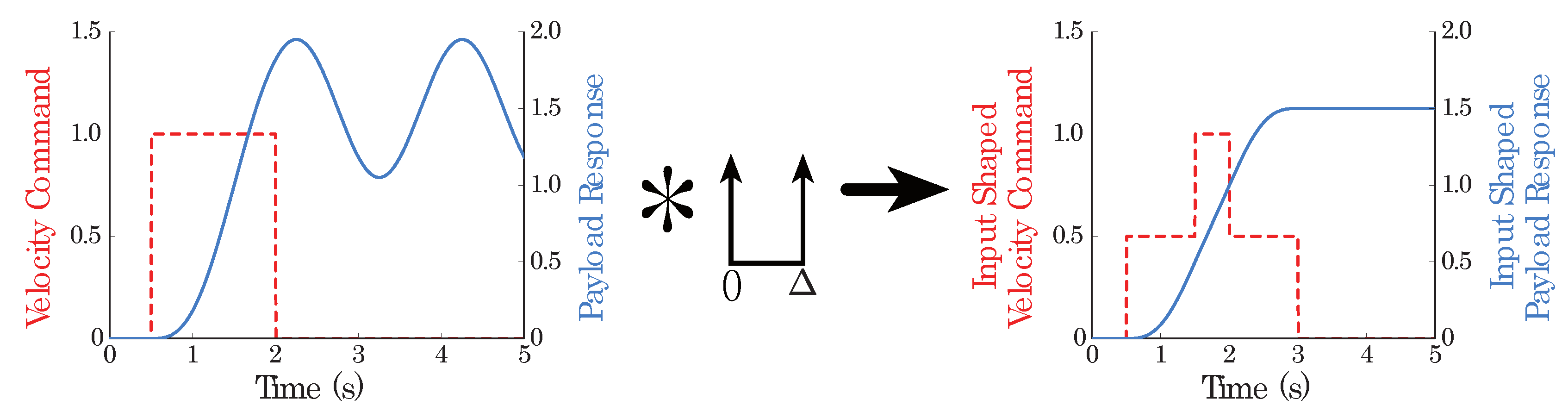
Figure 2.
(a) Physical Representation of the Mass-Spring-Damper System under gross sliding friction force.(b) Block Diagram Representation of the System Dynamics by the Lapace model.
Figure 2.
(a) Physical Representation of the Mass-Spring-Damper System under gross sliding friction force.(b) Block Diagram Representation of the System Dynamics by the Lapace model.
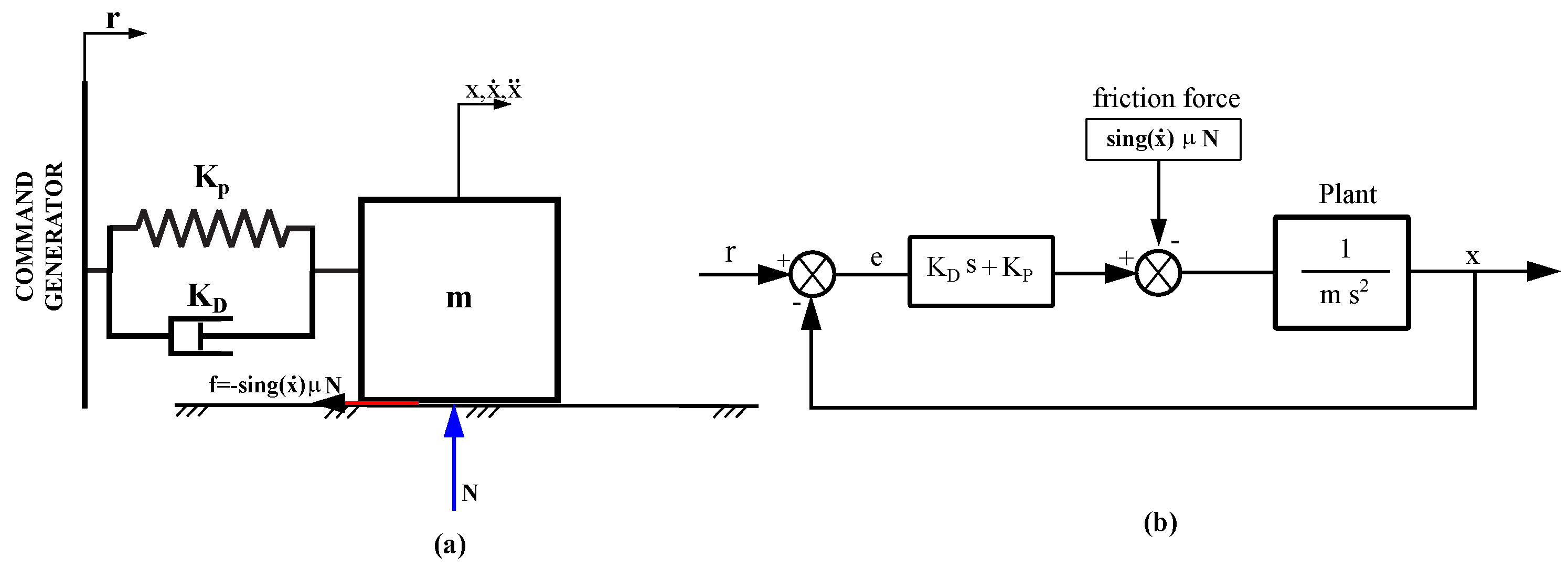
Figure 3.
Response of the mass-spring system under gross-slip friction, without the derivative damper action, to a non-zero initial position.Conditions:
Figure 3.
Response of the mass-spring system under gross-slip friction, without the derivative damper action, to a non-zero initial position.Conditions:
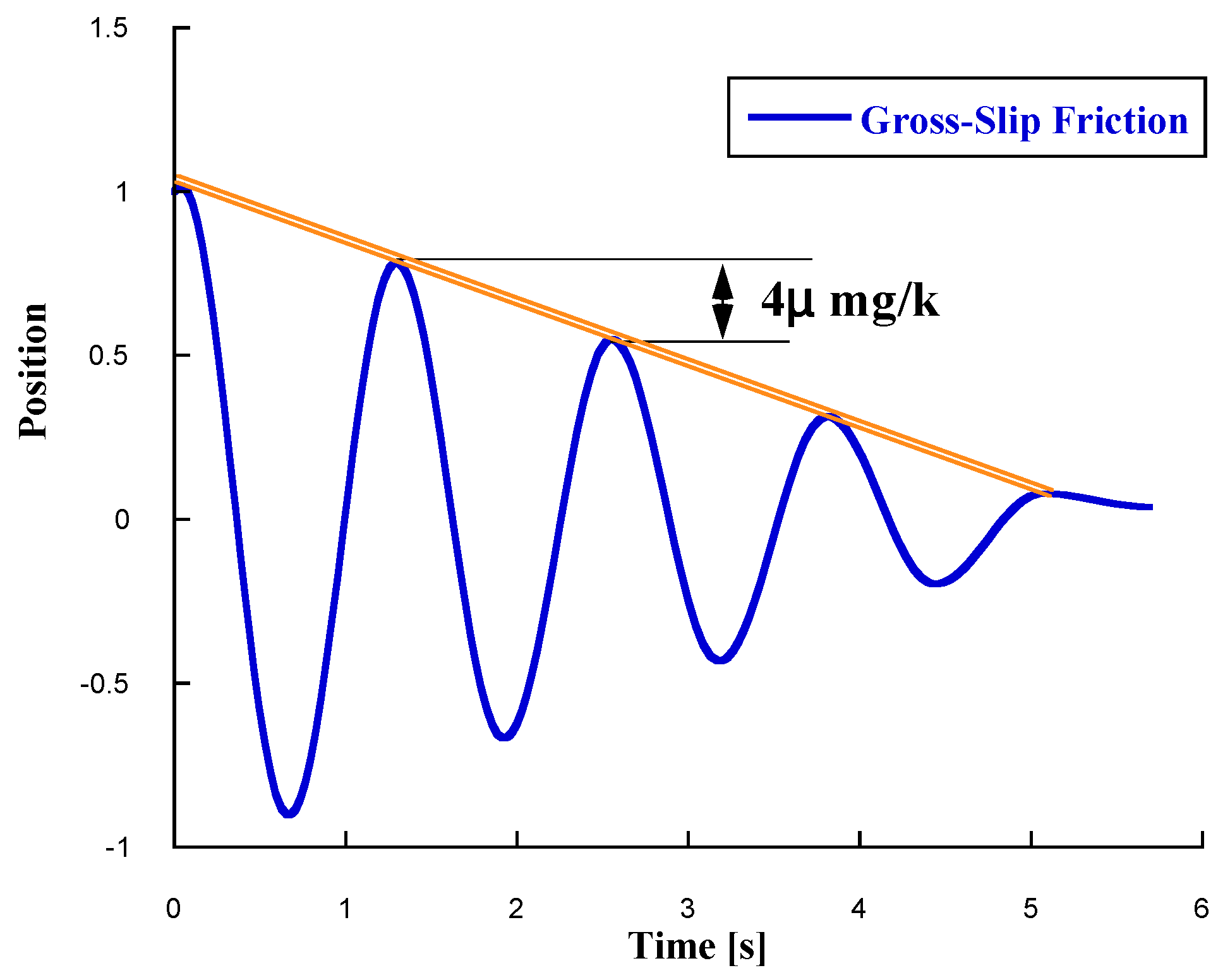
Figure 4.
Elastic rolling contact of a cylinder rolling freely on a plane under normal load P.
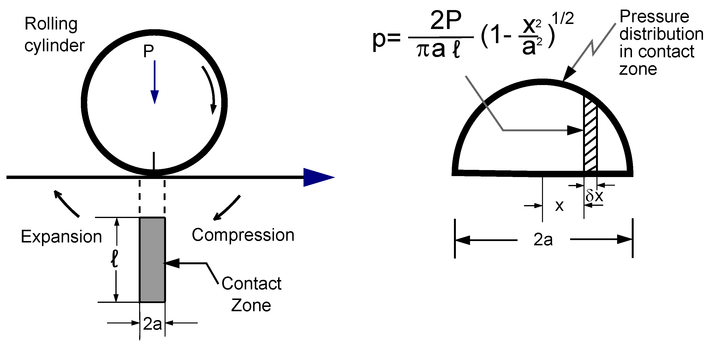
Figure 5.
(a) Reference model of a two-mass and spring system undergoing rolling friction. (b) Impulse response of the rolling disk, showing the nearly undamped x-position of the mass center.
Figure 5.
(a) Reference model of a two-mass and spring system undergoing rolling friction. (b) Impulse response of the rolling disk, showing the nearly undamped x-position of the mass center.
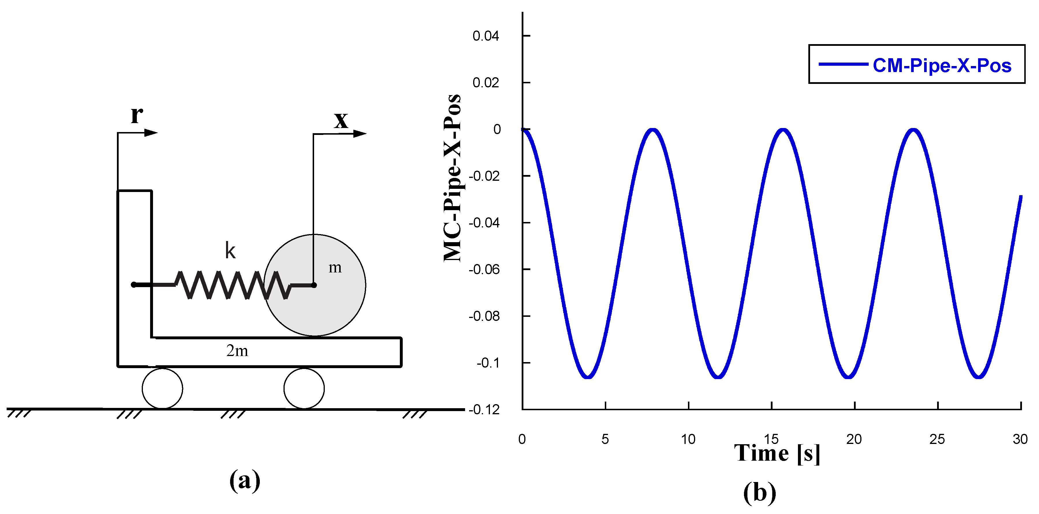
Figure 6.
(a) The System model (b) Corresponding Free Body Diagrams.
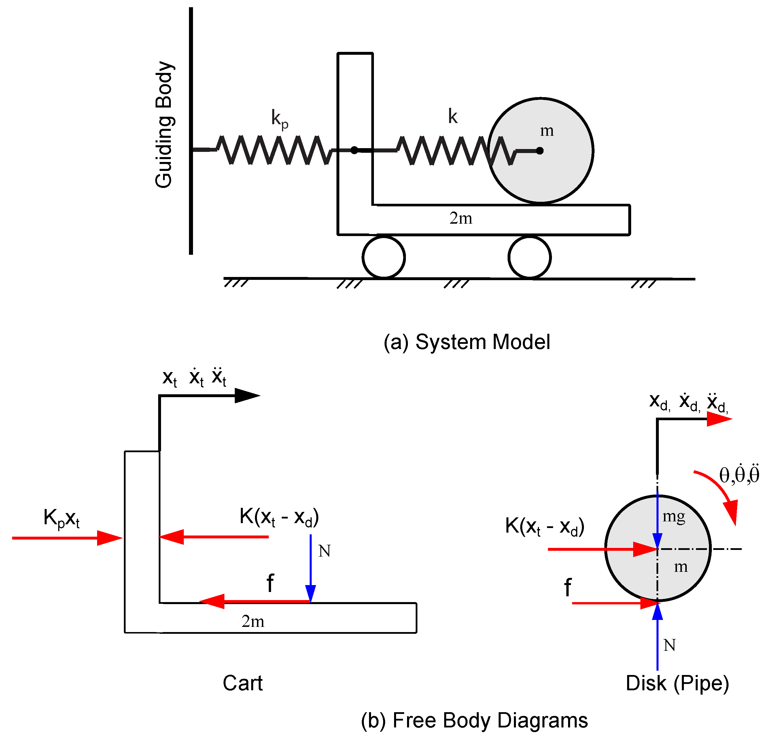
Figure 7.
Simscape Mechanical Explorer Sketch of the system showing the frames used in the model.
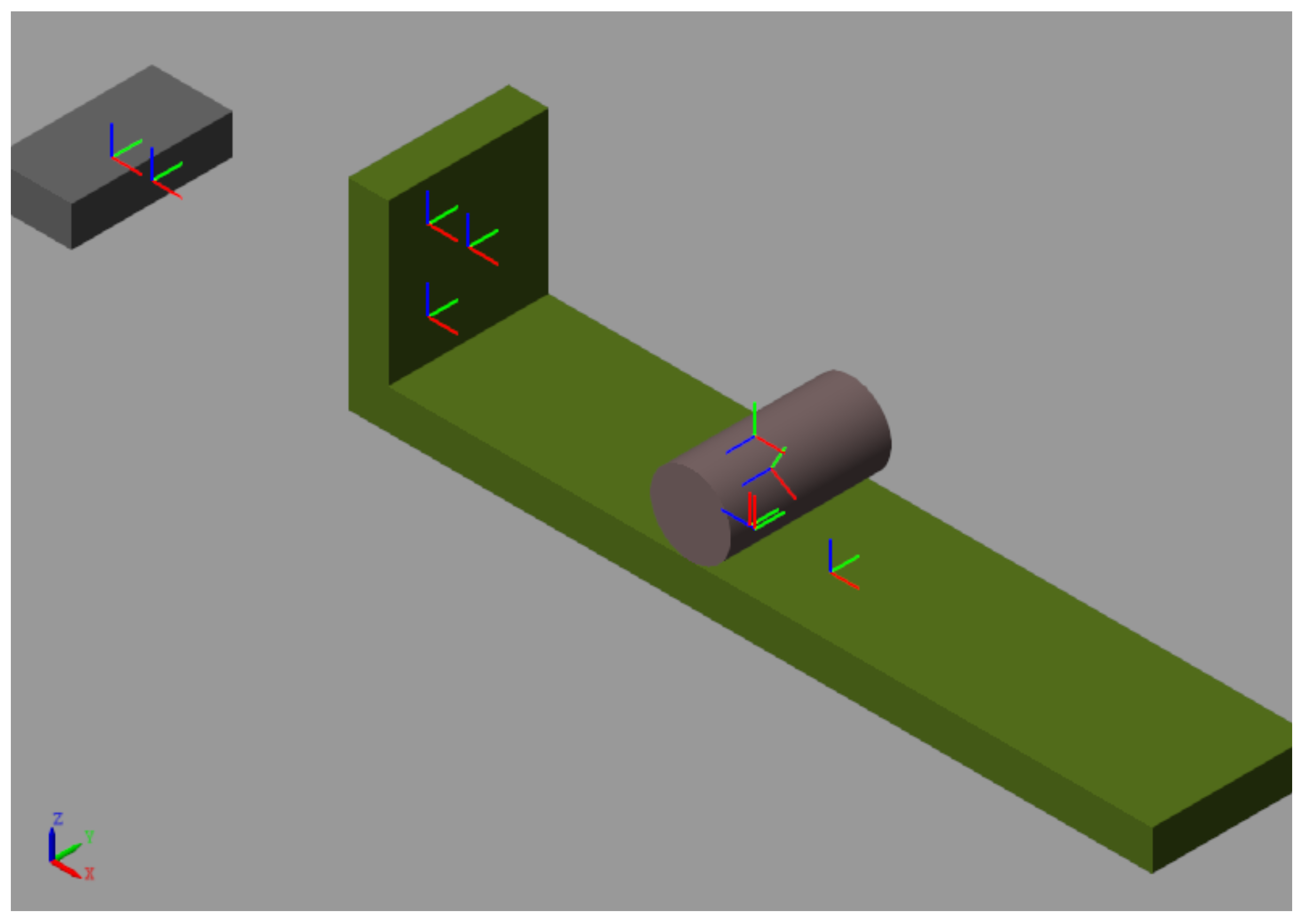
Figure 8.
Simscape(Matlab) Multibody Model of the System showing interconnected bodies by the kinematics joints plus a large number of important multibody formalism by rigid frames transforms plus bodies and joints customization.
Figure 8.
Simscape(Matlab) Multibody Model of the System showing interconnected bodies by the kinematics joints plus a large number of important multibody formalism by rigid frames transforms plus bodies and joints customization.
Figure 9.
FFT of the signal corresponding to the abscissa position of the center of mass of the pipe. (a) Low frequency component value 0.079998 [Hz] (b) High frequency component 0.159997 [Hz]
Figure 9.
FFT of the signal corresponding to the abscissa position of the center of mass of the pipe. (a) Low frequency component value 0.079998 [Hz] (b) High frequency component 0.159997 [Hz]
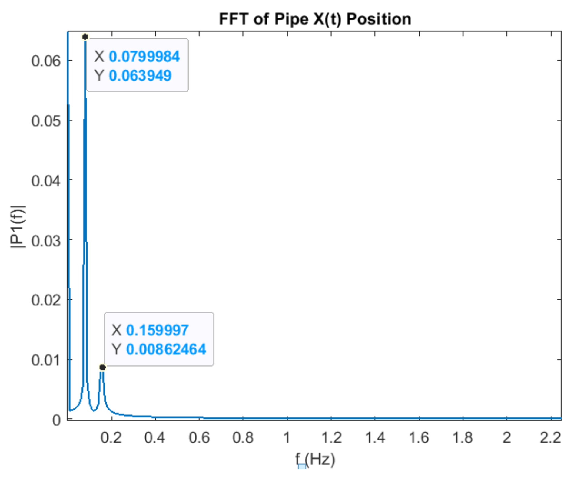
Figure 10.
Convolved Two-Mode ZVD-ZVD Shaper for 0.07998 and 0.159997 Hz undamped frequencies.
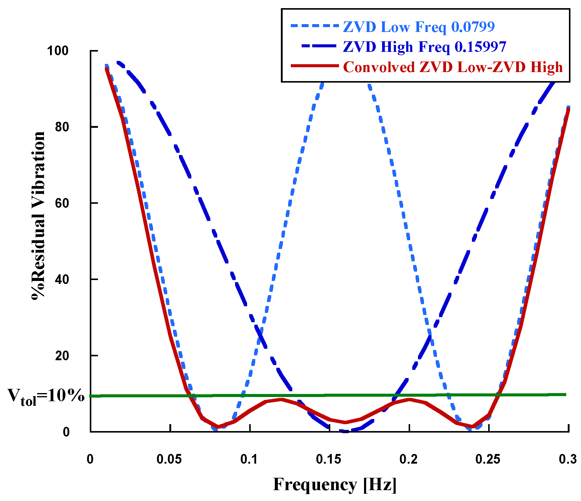
Figure 11.
Two-mode input shaper by simultaneous constraints for 0.07998 and 0.159997 [Hz] and 0.0.
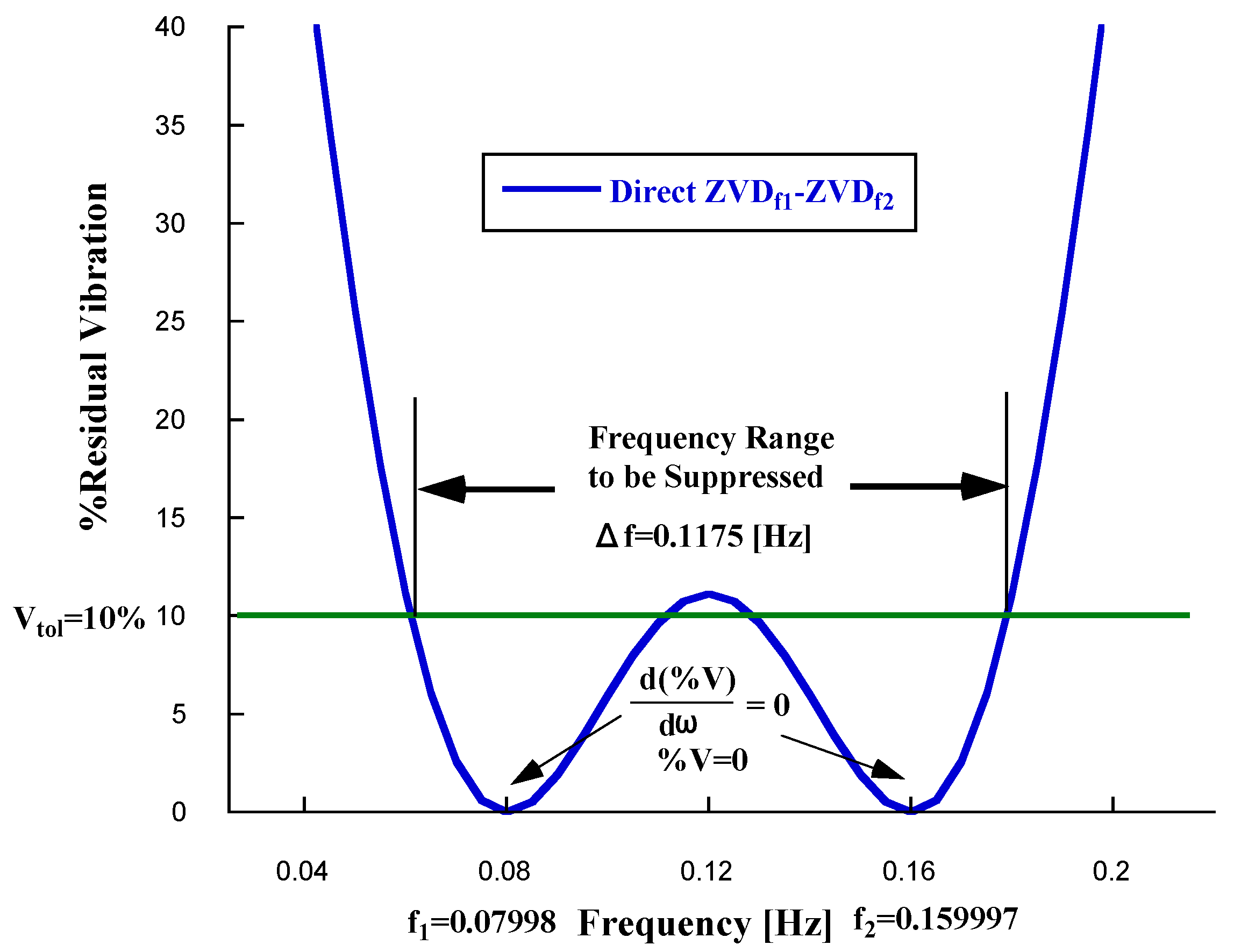
Figure 12.
Trapezoidal Input Motion. Conditions: the ramp up last for 17 [s]. (a) Unshaped Input Motion (b) Direct ZVD-ZVD Shaped Input Motion. Conditions: ramp-up last for :33[s]
Figure 12.
Trapezoidal Input Motion. Conditions: the ramp up last for 17 [s]. (a) Unshaped Input Motion (b) Direct ZVD-ZVD Shaped Input Motion. Conditions: ramp-up last for :33[s]
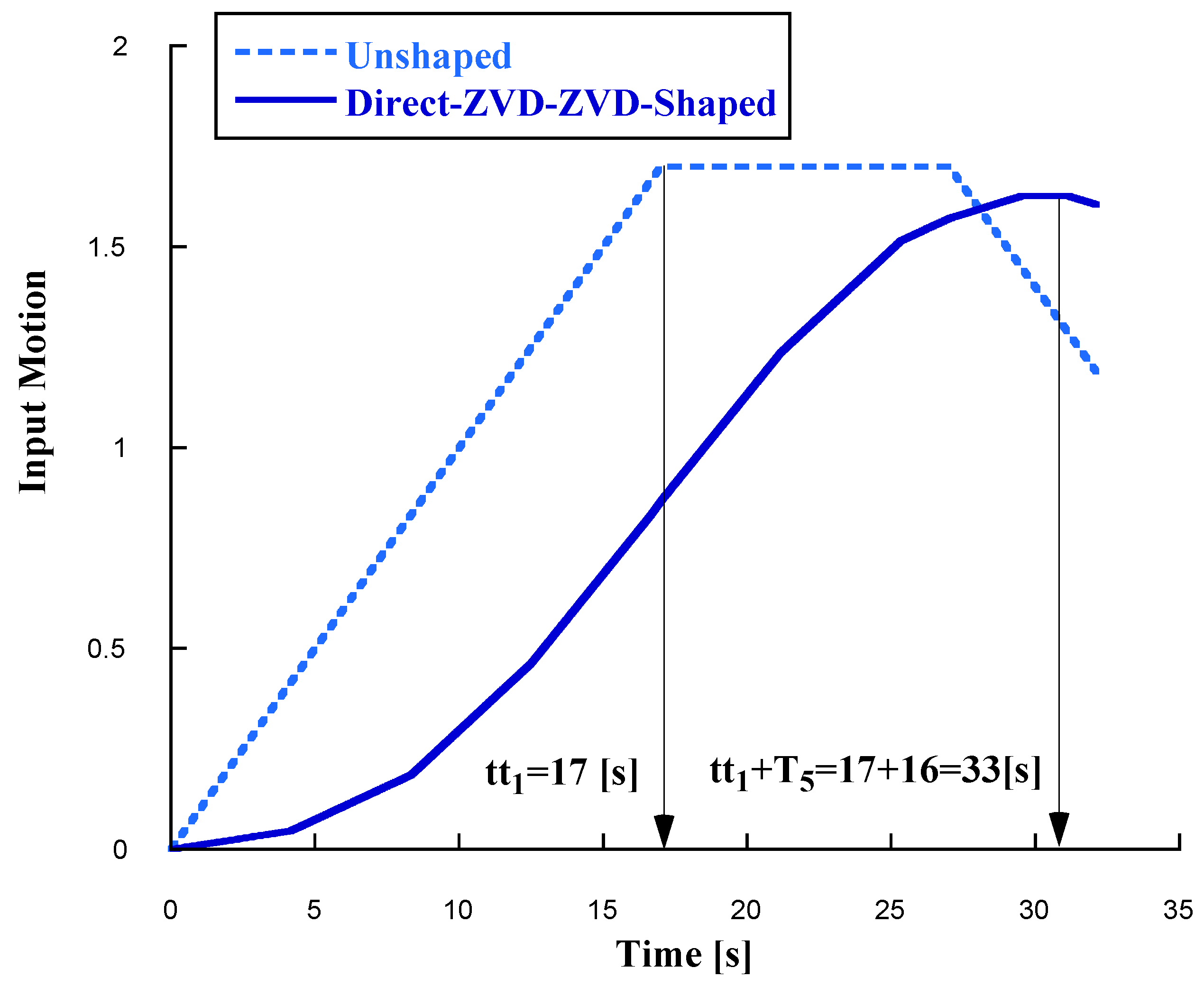
Figure 13.
Multibody Model Pipe Mass Center X-Position responses to Trapezoidal Input Motion profile with 12 seconds ramp up. (a) Pipe Mass Center X-Position Unshaped Response (b) Pipe Mass Center X-Position Shaped response for Direct ZVD-ZVD Shaped Input Motion
Figure 13.
Multibody Model Pipe Mass Center X-Position responses to Trapezoidal Input Motion profile with 12 seconds ramp up. (a) Pipe Mass Center X-Position Unshaped Response (b) Pipe Mass Center X-Position Shaped response for Direct ZVD-ZVD Shaped Input Motion
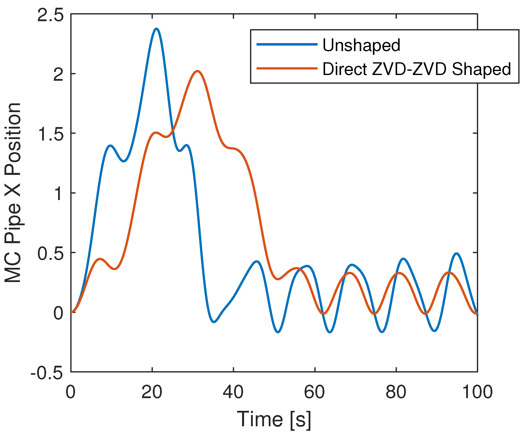
Figure 14.
Trapezoidal Input Motion. Conditions: the ramp up last for 20 [s]. (a) Unshaped Input Motion (b) Convolve ZVD-ZVD Shaped Input Motion
Figure 14.
Trapezoidal Input Motion. Conditions: the ramp up last for 20 [s]. (a) Unshaped Input Motion (b) Convolve ZVD-ZVD Shaped Input Motion
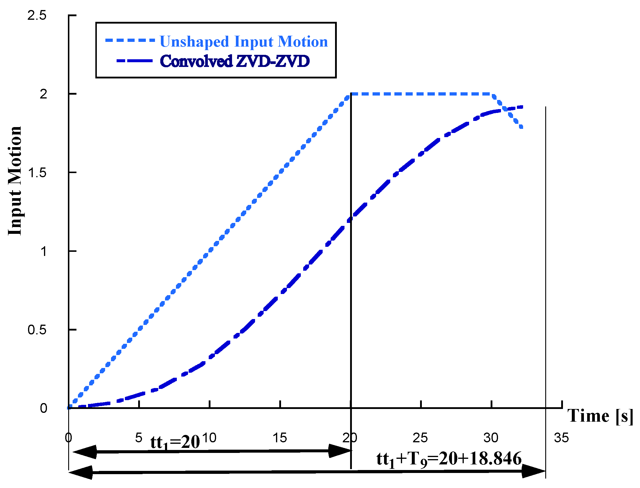
Figure 15.
Experimental Trapezoidal Input Motion profile Responses. (a) Pipe Mass Center X-Position Unshaped Response (b) Pipe Mass Center X-Position for Convolved ZVD-ZVD Shaped Response
Figure 15.
Experimental Trapezoidal Input Motion profile Responses. (a) Pipe Mass Center X-Position Unshaped Response (b) Pipe Mass Center X-Position for Convolved ZVD-ZVD Shaped Response
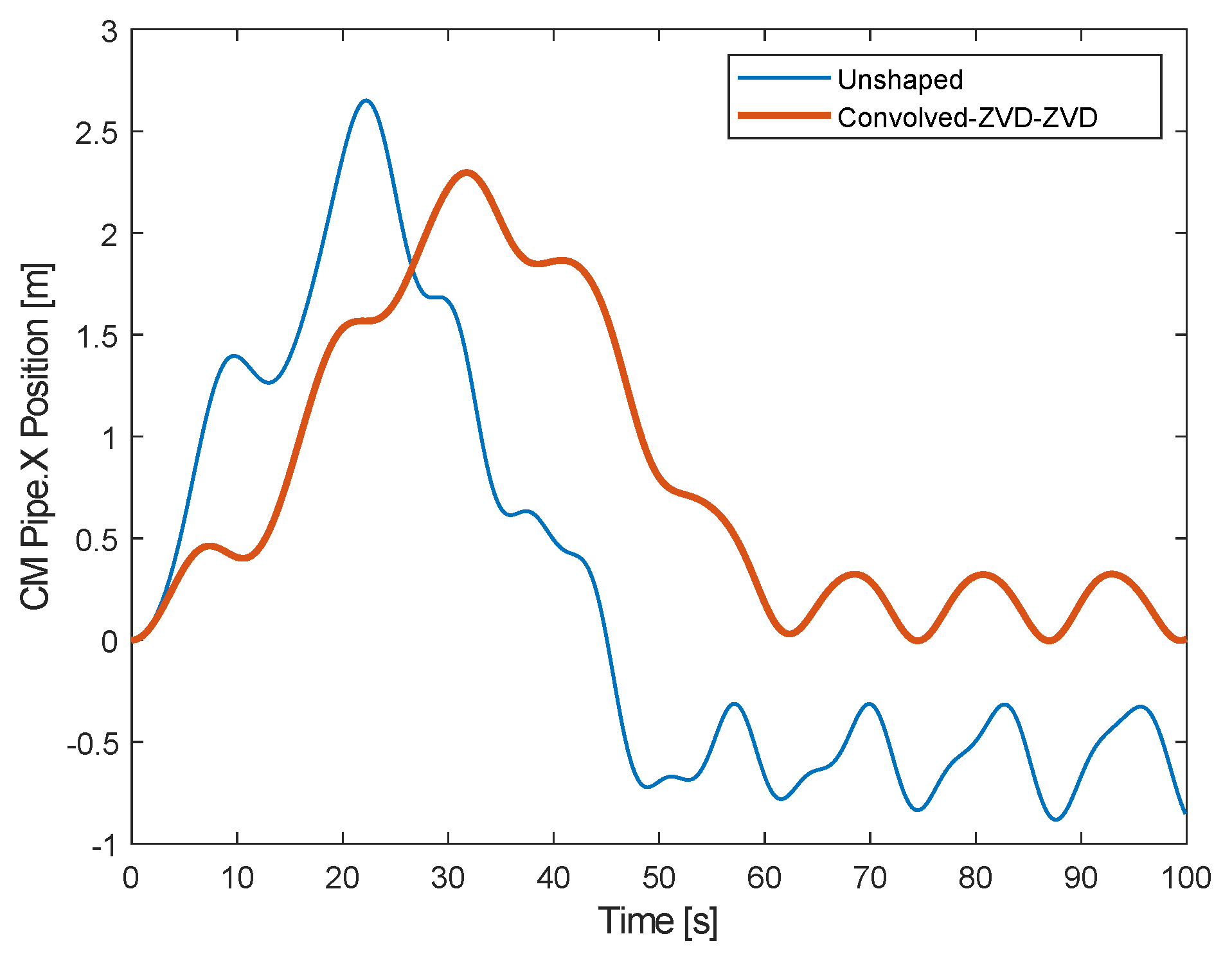

Table 1.
System natural frequencies analytical expressions and corresponding numerical values.
| expression | numerical value | numerical frequency [Hz] |
|---|---|---|
| = | ||
| = |
Table 2.
Normal Force customized parameters.
| Method 1 | Stiffness | Damping |
|---|---|---|
| Transition Region With | ||
| Smooth Spring Damper | 1e6 N/m | 1e3 N/(m/s) |
1 Transition Region With: 1e-4m.
Table 3.
Friction Force customized parameters.
| Method 1 | Coefficient Of Static friction | Coeficient Of Dynamic Friction |
|---|---|---|
| Smooth Stick Slip | 0.3 | 0.3 |
1 Critical Velocity 1 m/s.
Table 4.
Convolved and Direct Two-Mode Robustness.
| Two-mode Shaper | Frequency Range | Width and Percentage % |
|---|---|---|
| Convolved | [0.05 0.25] Hz | 0.20 Hz - 100% |
| Direct 1 | [0.0611 0.1786] Hz | 0.1175 Hz - 58.75% |
1 Simultaneous constraints.
Table 5.
Z Prismatic Primitive Joint Actuation.
| Force | Motion |
|---|---|
| Automatically Computed | Provided by Input |
| Follower on Base | Resolution Frame Base 1 |
1 Mode Configuration Normal.
Table 6.
Comparison of Unshaped and Direct ZVD-ZVD Responses.The ramp up last for 17 [s]
| Input | min | max | median | mode | std |
|---|---|---|---|---|---|
| Unshaped | -0.1686 | 2.376 | 0.3173 | -0.1686 | 0.6573 |
| Direct ZVD-ZVD | -0.01324 | 2.02 | 0.3289 | -0.01324 | 0.6174 |
Table 7.
Comparison of Unshaped and Convolved ZVD-ZVD Responses. Ramp up last for 20 [s]
| Input | min | max | median | mode | std |
|---|---|---|---|---|---|
| Unshaped | -0.8821 | 2.651 | -0.3299 | -0.8821 | 1.024 |
| Convolved ZVD-ZVD Shaped | -0.0033 | 2.297 | 0.4213 | -0.00333 | 0.7322 |
Disclaimer/Publisher’s Note: The statements, opinions and data contained in all publications are solely those of the individual author(s) and contributor(s) and not of MDPI and/or the editor(s). MDPI and/or the editor(s) disclaim responsibility for any injury to people or property resulting from any ideas, methods, instructions or products referred to in the content. |
© 2025 by the authors. Licensee MDPI, Basel, Switzerland. This article is an open access article distributed under the terms and conditions of the Creative Commons Attribution (CC BY) license (http://creativecommons.org/licenses/by/4.0/).
Copyright: This open access article is published under a Creative Commons CC BY 4.0 license, which permit the free download, distribution, and reuse, provided that the author and preprint are cited in any reuse.


