Optimizing Deep Learning Models for Climate-Related Natural Disaster Detection from UAV images and Remote Sensing Data

1. Introduction

According to the 2021 Intergovernmental Panel on Climate Change (IPCC) report, every continent worldwide has exhibited a rise in average temperatures due to anthropogenic climate change [1,2]. Heat waves which developed before the industrial revolution with a probability of 1 in 10, will now occur 2.8 times more often and be even hotter than before [2]. Globally, thirty seven percent of mortalities due to overheating were caused by global warming [3]. Climate change has been made more apparent through the intensity of extreme weather events such as heatwaves, hurricanes, heavy precipitation, flooding, etc. [1].

Flooding alone has led to over $610 billion in damages [1,4]. Research studies have demonstrated that the rising intensity of floods has been driven by climate change [1,5,6,7,8,9]. This project addresses the detection of extreme weather, natural disasters, and the resulting environmental degradation of land by utilizing AI, ML, and DL techniques.

Desertification can be described as the degradation of the land in arid, dry sub-humid, semi-arid regions due to climate change and other anthropogenic activities [10,11]. Global warming accelerates desertification [10,12]. The variations to weather patterns caused by climate change exacerbates desertification [13]. Approximately 25% of the land surface worldwide is being impacted by desertification [10,11,14]. Research modeling has predicted that the (moderate – very high) risk of desertification will rise by twenty three percent before 2100 in their high greenhouse gas emissions scenario [10].

Other research studies have delved into AI detection of such extreme weather events and natural disasters as flooding, etc. [15,16,17,18,19]. In a study by Daniel Hernández et al., their research group developed an AI pipeline to detect natural disasters such as flooding [15]. Albandari Alsumayt et al. designed the Flood Detection Secure System (FDSS) which utilized drones for image classification of flooding events while keeping the data secure [16]. Naili Suri Intizhami et al. presents their flood area dataset containing images of flooding in Indonesia and color labeled annotation for computer vision research on flooding identification [17]. Fatma S. Alrayes et al. has developed their own AISCC-DE2MS technique for emergency disaster monitoring by drones which includes encryption and image classification functionality [18]. R. Karanjit et al. introduced their novel dataset, Flood image (FloodIMG) in combination with DL techniques to classify flooding events [19]. Our research project seeks to accurately detect natural disasters such as flooding and desertification. Desertification has become an increasingly critical matter, which has rarely been addressed previously in deep learning AI disaster detection projects from images.

Tools to accurately detect and predict natural disasters are needed to prevent and lower the property damages along with the number of mortalities. Significant progress has been made in recent years in AI detection of natural disasters. These methods often use remote sensing, satellite imagery, and/or unmanned arial vehicle (UAV) images in their training dataset [15,16,18,19]. Surveillance tactics are required to notify the public in adequate time of impending danger from extreme weather events.

For decades now, satellites have been monitoring and providing beneficial observations of land & sea conditions [20] at moderate resolution and at coarse resolution. In recent years, research studies have been able to utilize high-resolution satellite images of less than five meters [21]. UAV imagery has also begun to play an increasing role in AI research studies in the environmental science/agriculture fields [22,23,24]. Dilmurat et al. monitored changes in crops through UAV LiDAR and hyperspectral imaging to accurately forecast maize yield with their H20 Automated Machine Learning framework [22]. Damini Raniga et al. presented a workflow of AI detection and monitoring of the health condition of the delicate vegetation in East Antarctic’s protected area by utilizing non-invasive UAV images [23]. Andrea Santangeli et al. was able to effectively combine UAV thermal imaging with AI detection to precisely identify bird nests lying on agricultural fields with the intent that their tractors should avoid the ground-level bird nests [24]. UAVs, also known as drones, have been utilized for flood image classification/detection purposes, as well [15,16,18]. For instance, Daniel Hernández et al., proposed an AI-based pipeline, taking drone images of floods as input, extracting key features, reducing the complexity of the feature data, grouping unlabeled images by similarity, and then sending prototypes of the clusters for manual labelling of drone images by natural disaster first responders [15]. UAV imagery has a higher spatial resolution than satellite imagery and can often offer greater accuracy in image classification [25].

UAV images have many advantages besides high-resolution imaging including the ease of transportation and deployment [21]. Drones can be used during cloudy weather conditions and still produce quality aerial images [26]. UAVs used for Low Altitude Sensing Systems (LARS) offer enhanced flexibility [26]. Drones cannot yet rival the amount of spatial area that satellites are able to cover but UAV data could potentially complement and augment satellite data [21].

Several research studies have effectively combined both UAV and satellite remote sensing imaging for classification/detection purposes [19,21,27]. Dash et al. performed a controlled study on the effects of herbicide on P. radiata through analysis of both UAV and satellite remote sensing imaging [21]. Karanjit et al. compiled images of flooding from a variety of sources: Google Search, Twitter, DOT traffic cameras, GitHub, USGS, etc. with huge variations in resolution size for AI-driven flood detection [19]. Marx et al. utilized Landsat satellite data in combination with UAV images of remote areas uncaptured by high resolution satellite imagery to document deforestation and reforestation events [27].

An open-access data site, Kaggle, has become well-known and utilized in research studies [28,29,30,31,32,33]. Kaggle datasets containing medical imaging have been used in disease detection [28,29,30,32,33]. Hassan et al. utilized 3 benchmark datasets to present their novel multi-stage deep neural network architecture for the detection of Alzheimer’s disease [28]. Land use/land categorization articles have benefited from Kaggle datasets, as well [34,35]. Kwenda et al. introduces a hybrid approach combining deep neural networks and ML algorithms trained on the deep globe challenge dataset for the purposes of image segmentation of satellite images into forest versus non-forest regions [34]. Natural Learning Processing (NLP) research has also made use of Kaggle datasets [36]. Kaggle datasets can be found in cybersecurity research [37]. Amnah Albin Ahmed et al. utilized ensemble and DL models trained on the Android Ransomware Detection dataset for detection of such cyberattacks [37]. Kaggle competitions have even been studied and analyzed in research journals [31,38]. Souhaib Ben Taieb and Rob J. Hyndman analyzed the approach used by their team in the Load Forecasting track of the Kaggle Global Energy Forecasting Competition [38].

This research focuses on AI-based flood detection. Previous studies have utilized Kaggle datasets for flood detection [17,19]. Naili Suri Intizhami et al. posted one such open access dataset [17]. Intizhami et al. utilized images posted on social media of flooding in South Sulawesi Indonesia [17]. With these images, Intizhami et al. built their own dataset color annotated with 6 different classes for use by ML/DL models for image segmentation purposes [17]. This project trained ML/DL models on our Climate Change Dataset compiled from various related Kaggle datasets.

The aim of this project was (1) to harness the capabilities of AI, ML, DL, and Data Science to tackle complex environmental issues, (2) to utilize existing aerial images to build AI/ML models to detect land degradation from extreme weather events such as flooding or desertification (3) to demonstrate the ability of AI/ML to be used for humanitarian efforts such as research on climate change crisis problems. To achieve these goals a dataset was compiled of aerial images, machine learning models were built, transfer learning was utilized, and the best performing ML model was optimized. We hypothesize that DL image classification techniques can detect climate change related natural disasters, such as flooding & desertification, based on aerial images of the given area with an accuracy surpassing seventy percent.

2. Materials and Methods

In this section, we will first introduce the dataset we collected for this work, followed by the data pre-processing, model building and selections, then experiment set-up and evaluation metrics.

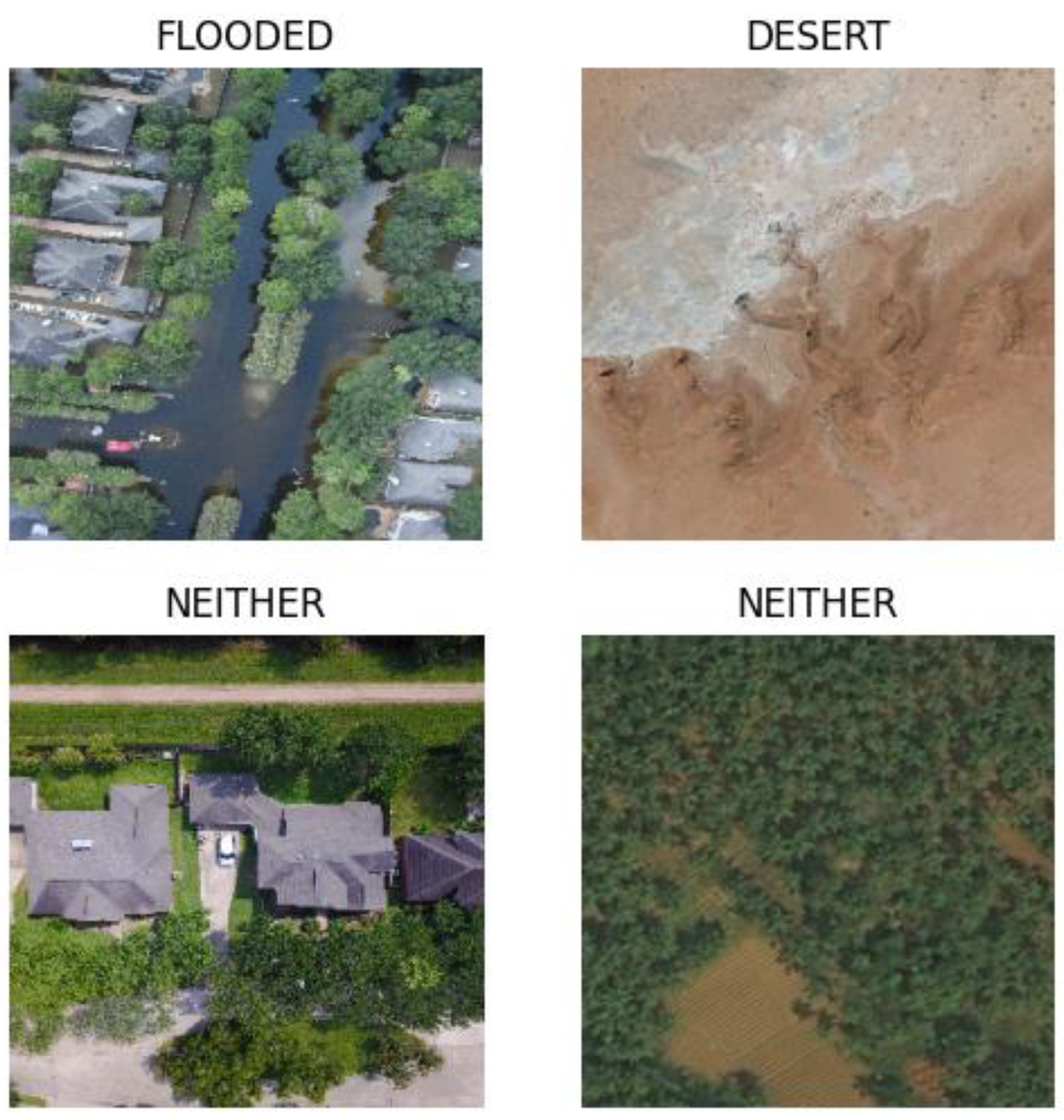
2.1. Compiling the Climate Change Dataset

We will now explain how our dataset was assembled. Over 6.3K aerial images from unmanned aerial vehicles and satellite images were collected and used to form the compiled Climate Change Dataset totaling 6,334 images. Multiple datasets from the open-source data site, Kaggle [39], were utilized including: Louisiana Flood 2016 [40], FDL_UAV_flood areas [41], Cyclone Wildfire Flood Earthquake Database [42], Satellite Image Classification [43], Disaster Dataset [44], Aerial Landscape Images [45], Aerial Images of Cities [46] & Forest Aerial Images for Segmentation [47].

The Climate Change Dataset contains 3 categories: Flooded, Desert, and Neither. Both flooding and desertification are climate change related natural disasters. Neither category represents those images which are neither flooding nor desertification. The Flooded category contains over 2K aerial images of flooded residential areas (2,338 images). Pertinent images for the Flooded category were selected from: Louisiana Flood 2016 [40], FDL_UAV_flooded areas [41], Cyclone Wildfire Flood Earthquake Database [42], and the Disaster Dataset (subset comprehensive disaster dataset / water disaster & the disaster dataset final / flood subset) [44].

The Desert category contains over 2K aerial images of desert areas (1,931 images). Relevant images for the Desert category were selected from: Satellite Image Classification (Desert subset) [43] and Aerial Landscape Images (Desert subset) [45]. The Neither category contains over 2K aerial images of non- flooded residential areas and non-flooded forested areas (2,065 images).

Table 1 shows the image count for each data source. Qualifying images were selected from: Louisiana Flood 2016 [40], FDL_UAV_flooded areas [41], Aerial images of Cities (Residential subset) [46], Disasters Dataset (neutral images subset) [44] and the Forest Aerial Images for Segmentation [47]. These datasets contributed to the Neither category.

The image dimensions include variable sizes ranging from (224 X 224 pixels) to ( over 1000 pixels X over 1000 pixels). Both jpeg and png image formats were used in the dataset. Representative images can be seen in Figure 1.

Images from the Climate Change Dataset were screened and selected through a vigorous quality control process. Images were filtered to screen out: non-aerial images, logos, borders, and extremely blurry images. The datasets were manually perused and subjected to this quality control screening. Only images related to their appropriate category remained within the Climate Change Dataset.

2.2. Preprocessing and Model Initiation

During preprocessing, the images from the Climate Change Dataset were resized to 64 X 64 pixels to fit the CNN model we built. The 64 X 64 pixels image size was chosen for faster ML run speed. Alternatively, for the transfer learning models, the images were resized to 224 X 224 pixels instead to fit those models. Next, the dataset was split into the training set (80%) and testing set (20%). The Climate Change Dataset, following these preprocessing steps, was then loaded into our 4 ML models.

2.3. VGG16 Network Model

In this section and in the next few sections, we will discuss the 4 ML models utilized in our study. VGG16 [48] was chosen for its reputation as a high performing ML model for image classification. VGG refers to the Visual Geometric Group from Oxford University where Simonyan and Zisserman developed the VGG network model [48]. The VGG-16 model included 3 fully connected layers and 13 convolutional layers. We used the VGG-16 model pre-trained on the ImageNet dataset. The VGG network model became well known when the model received one of the top prizes for the ImageNet Large Scale Recognition Challenge in 2014 [49].

2.4. DenseNet201 Network Model

DenseNet [50] was recommended by a colleague in AI research for the ML model’s high testing accuracy. DenseNet201 [50] network model is a Dense Convolutional network. The dense connections lead to higher testing accuracy when compared to other network models. Each layer of the DenseNet [50] model receives input from all preceding layers in a feed-forward fashion [50]. Features from the various layers of the DenseNet [50] model are concatenated together which encourages reuse of learned features.

DenseNet [50] was further optimized to increase the testing accuracy for natural disaster detection. Numerous layers were added to the model architecture. These layers are discussed below.

2.4.1. Data Augmentation Layer

Keras preprocessing experimental layers adjust images for better accuracy in predictions of new data. Data augmentation increases the diversity of your dataset [51]. Several random transformations are applied to the images to accomplish this task. We used Keras preprocessing experimental layers for data augmentation purposes. Random contrast and random zoom transformations were applied to our dataset of images. Random contrast was set to 0.3 and random zoom was set to 0.1.

2.4.2. Rescaling Layer

A rescaling layer was added to the ML model architecture. The images were normalized by rescaling the original pixel values to values between 0 and 1. The empirical method was used which divides the pixel intensity value by 255. Normalizing the pixel intensity through the empirical method yields higher testing accuracies for ML classification [52].

2.4.3. Global Average Pooling Layer

A Global Average Pooling (GAP) layer was added to our DenseNet [50] model. The GAP layer takes the average of the feature map for each category. This layer is useful in avoiding overfitting [53].

2.4.4. Dropout Layer

A dropout layer was also added to reduce overfitting of our DenseNet [50] model to the data. A portion of neurons was excluded to promote variations in the data. A dropout rate of 0.2 was selected. The dropout layer enhances the capability of our DenseNet [50] model to generalize new, never seen, data [28].

2.4.5. Fully Connected Layer and Classifier

The fully connected layer (FC) is a key, integral part of convolutional neural networks [54]. For shallow CNN’s, the FC layer is required since the features found by the last convolutional layer of a shallow CNN does not cover the entire spatial image [54]. Instead, only a portion of the overall image is being represented in the feature map. For FC layers, each neuron in the layer is connected to each neuron in the previous layer enabling high level feature extraction [28]. For our DenseNet [50] model, we used 3 FC layers containing 64, 64, and 3 neurons.

Located in the final layer, the SoftMax classifier is crucial for accurate image classification. The SoftMax classifier assigns a probability between 0 to 1 for each category, giving an indication of the confidence level of the model’s prediction [28]. The summation of probabilities totals 1.

2.5. ResNet50 Network Model

We utilized ResNet [55] in our Python model due to its history of outperforming in ML challenges. In 2015, the ResNet50 [55] network model received one of the top prizes in the ImageNet Large Scale Recognition Challenge. The ResNet50 [55] network model is a CNN containing 50 layers. The vanishing gradient problem leads to higher error rates in neural networks as the network becomes deeper [56]. This challenge was overcome with the skip connection technique incorporated into the ResNet50 [55] model. The skip connection creates a shortcut between layers in order to enable a direct connection to the output [56].

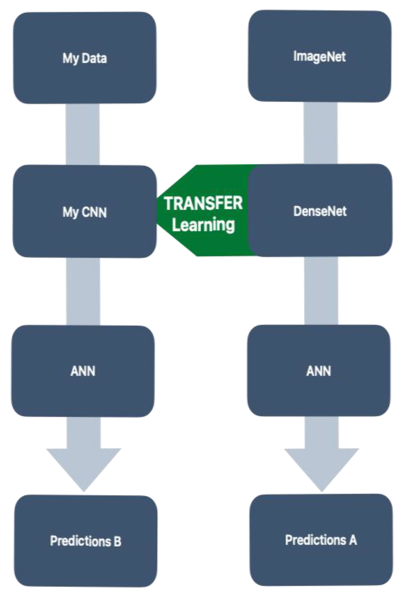
2.6. Transfer Learning Framework

ML models (VGG16 [48], DenseNet201 [50], ResNet50 [55]) pre-trained on the ImageNet dataset were utilized for our ML module. Features learned previously to make predictions were applied to this new problem of climate change related natural disaster detection. The transfer learning framework has been visualized in Figure 2. Transfer learning models have been well documented for yielding high testing accuracies on new datasets [29,47,49,56]. Our Climate Change Dataset was loaded into each of these pre-trained ML models. New predictions were then made utilizing transfer learning techniques. Three pre-trained ML models were compared: VGG16 [48], DenseNet201 [50], and ResNet50 [55].

2.7. Convolutional Neural Network (CNN) Model

We built our own rudimentary convolutional neural network (CNN) for the purposes of detecting climate change related natural disasters. A detailed review of layers utilized in ML models is given in the DenseNet201 Network section.

2.7.1. CNN Layers

A quick mention of the layers utilized in our CNN model will be revealed in this section. The CNN model we built contains:

• 1 rescaling layer
• 1 data augmentation layer
• 3 convolutional layers
• 3 pooling layers
• 1 drop-out layer
• 3 fully connected (FC) layers

The final layer utilizes a SoftMax classifier for image classification. The rescaling layer normalized the image data from the original pixel intensity values into values between 0 and 1. The empirical method was used when the original pixel intensity values were divided by 255. In the data augmentation layer, we selected random contrast at 0.3 and random zoom at 0.1. The convolutional layers took an initial input of 64 X 64 X 3 with ReLU activation. Detailed information on the pooling layers is given below. For the drop-out layer, we selected 0.4 to reduce overfitting and to improve testing accuracy. The three FC layers contained 32, 64, & 3 neurons each.

2.7.2. Pooling Layers

Three pooling layers were added to our CNN model. Average pooling was used for the first pooling layer. Average pooling calculates the average value for the given region [57]. Max pooling was used for the last two pooling layers. Max pooling selects the largest value for the given region. Both average pooling and max pooling are feature extraction techniques. The pooling layer takes the feature map from the previous layer and pools the data from small local regions to build a new feature map with reduced spatial dimension [57].

2.8. Experimental Set-Up

This section describes the hardware and software environment used to run the experiments with different ML Python modules. The running of Transfer Learning modules is memory intensive. For this reason, our ML module was run with Google Colab Tensor Processing Unit (TPU) high-RAM v2-8 cloud. Google Colab was used to:

• Collaborate online with code/feedback
• Accelerate our ML workload with Google GPUs/TPUs
• Utilize Google’s cloud computing resources.

The code was written in Python version 3.11.1. Tensorflow, Keras and Scikit-Learn ML libraries were installed and utilized throughout our ML module.

2.9. Evaluation Metrics

In this section, we explain the evaluation metrics used to measure the performance of our ML models while providing the pertaining formulas, as well [34]. We utilized the following metrics: Accuracy, Confusion Matrix, Precision, Recall, and F1-Score. The Confusion Matrix was chosen to visually display the performance of our ML models. The predicted and actual classifications were compared within the confusion matrices. These tables show true positives (TP), true negatives (TN), false positives (FP), & false negatives (FN). Accuracy calculates the fraction of correct predictions per total predictions made by the ML model. The accuracy formula is given in Equation (1).

$$Accuracy={\displaystyle \frac{TP+TN}{TP+TN+FP+FN}}$$

(1)

Recall, also known as sensitivity, calculates the fraction of positives predicted correctly by the ML model per total actual positives in the batch. The Recall measures the ML model’s capability of correctly identifying the total actual positive cases. The Recall formula is expressed in Equation (2).

$$Recall={\displaystyle \frac{TP}{TP+FN}}$$

(2)

Precision calculates the fraction of true positives per total positives predicted by the ML model. Precision is a measure of the quality of the ML model’s positive predictions. The Precision formula is given in Equation (3).

$$Precision={\displaystyle \frac{TP}{TP+FP}}$$

(3)

The F1 score measures a ML model’s performance based on the precision and recall values. This metric calculates the harmonic mean of the precision and recall values [34]. The F1 Score formula is provided in Equation (4).

3. Results

In this section, we provided our experimental results. We began by displaying the individual performance of our 4 ML models (VGG16 [48], CNN, ResNet50, DenseNet201 [50]) for climate change related natural disaster detection. A comparison of the 4 ML models was made. Optimization techniques were discussed. We demonstrate how performance was improved with optimization. Finally, we juxtaposed two of our highest performing ML models, ResNet50 and DenseNet201 [50]. Testing accuracies and testing loss were plotted for all 4 ML models. The testing set was used for validation purposes. Cross-entropy loss was calculated for the validation loss graphs.

3.1. Individual Model Performance

We demonstrate the performance of each single ML model by visually displaying each ML model’s testing accuracy, testing loss, and confusion matrix across 70 epochs. We used a batch size of 64.

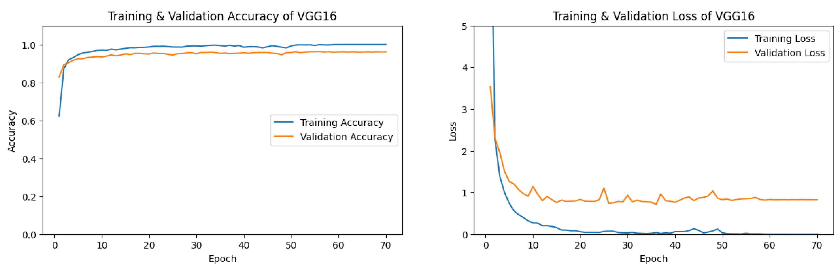
3.1.1. VGG16 Performance

Our VGG16 [48] model displayed a relatively high validation accuracy. A final validation accuracy of 96.13% was reached after 70 epochs, as seen in Figure 3.

The confusion matrix for VGG16 [48] can be seen in Figure 4. Label 0, the Desert category, showed the highest precision amongst categories. Less than 4% of the time, when an image from our Climate Change was inaccurately predicted, then that image was most likely from the Neither category, label 2.

In Table 2, the Desert category demonstrated an extremely high precision, recall, and F1-Score of 0.99. The Neither category had a lower recall and F1-Score of 0.94.

3.1.2. DenseNet Performance

Our DenseNet201 [50] Optimized model displayed extremely high validation accuracy of over 97% at epoch 1. The extremely low testing loss can be seen in Figure 5, as well. Our DenseNet201 [50] Optimized model reached 99.45% validation accuracy after 70 epochs.

All actual occurrences of label 0, the Desert Category, were accurately predicted by our DenseNet201 [50] Optimized model. As can be seen in the confusion matrix shown in Figure 6. Less than 1% of the time, when an image was predicted incorrectly, the image belonged to the Neither category, label 2.

The flooded category has one of the highest precision scores of 1.0 when classified by our DenseNet201 [50] Optimized model. Table 3, reveals the extremely high overall precision, recall, and F1-Scores for our DenseNet201 [50] Optimized model.

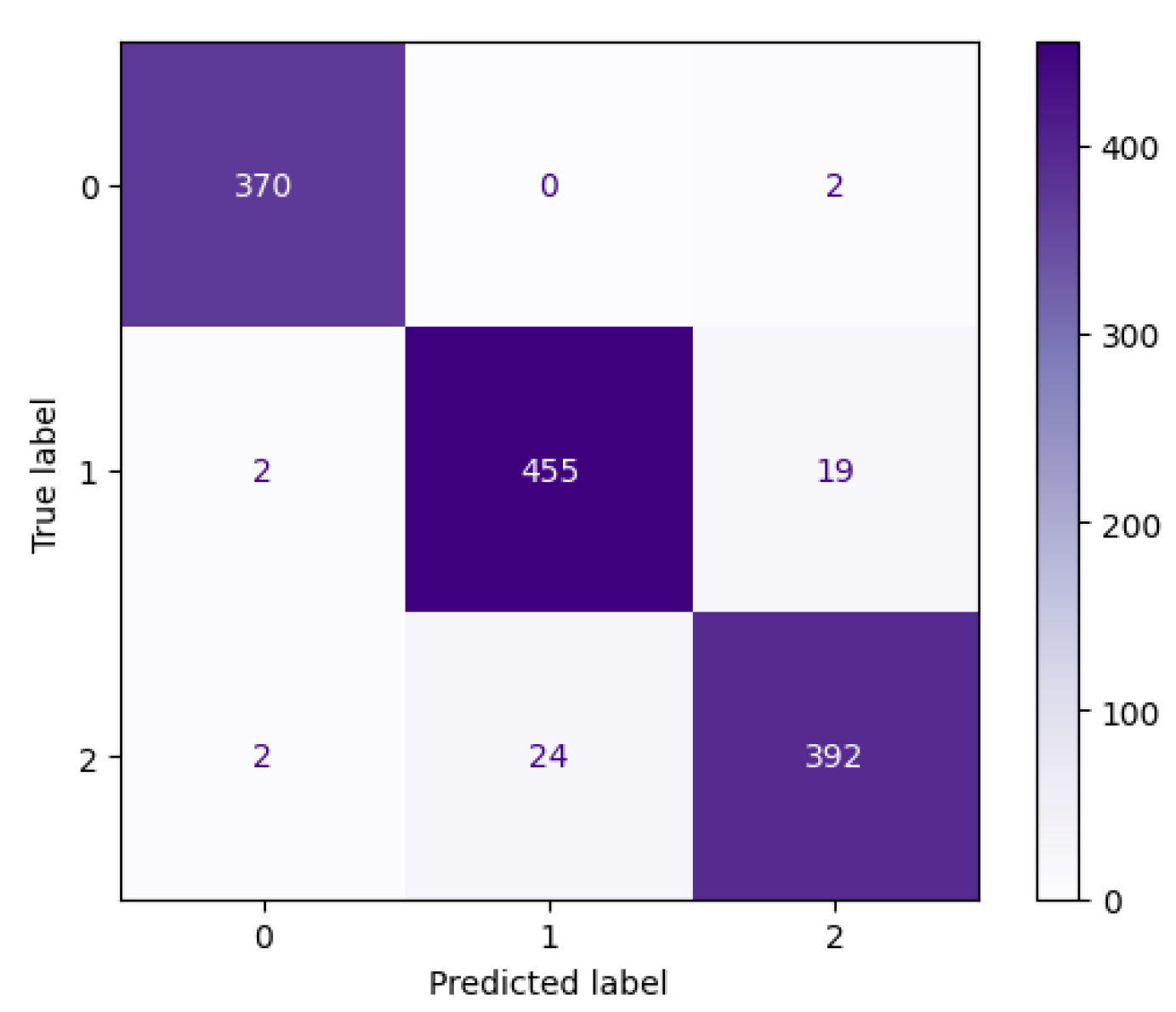
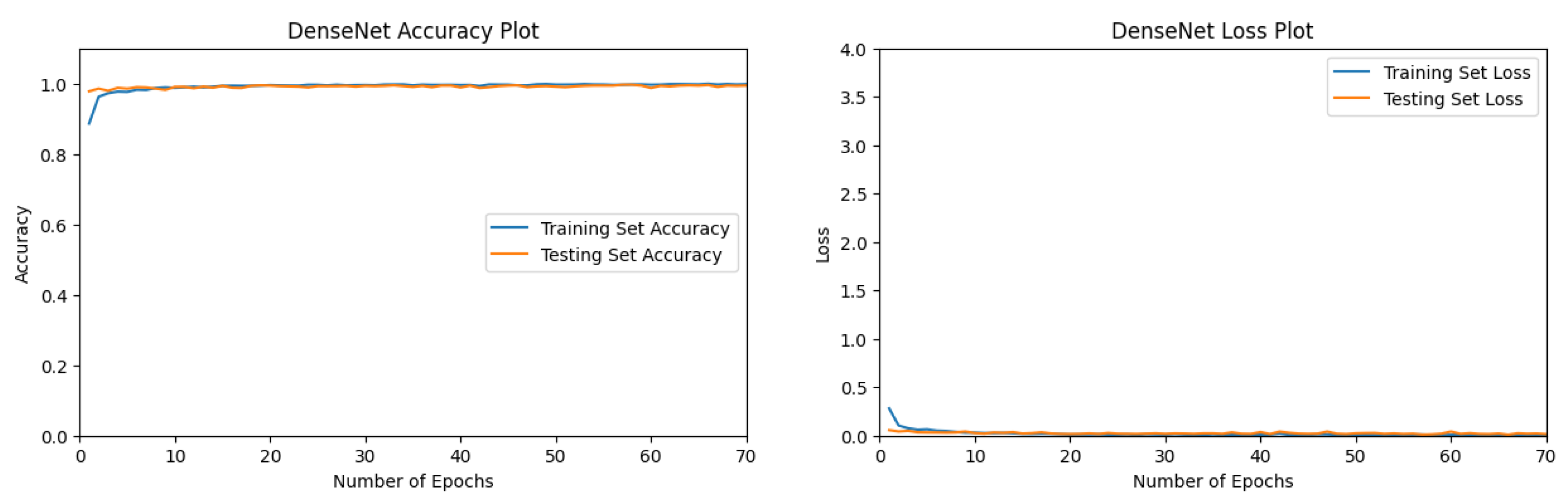
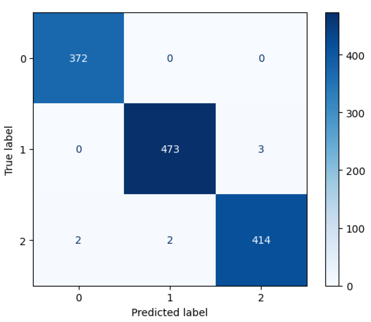
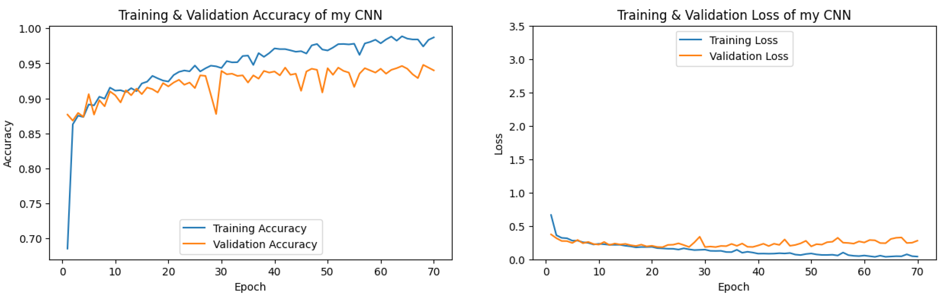
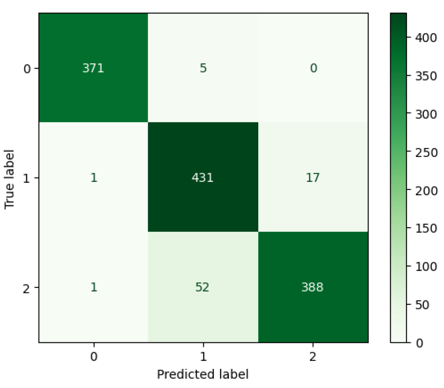
3.1.3. CNN Performance

Our CNN model was trained on our Climate Change dataset. As can be seen in Figure 7, our CNN model displayed 94.00% accuracy after 70 epochs.

The Desert category, label 0, was predicted by our CNN model with high accuracy, according to the confusion matrix seen in Figure 8. Six percent of the time, when an image from our dataset was incorrectly predicted then that image belonged to the Neither category, label 2.

According to Table 4, when compared to other categories, our CNN model demonstrated the highest scores for the Desert category with precision, recall, and F1-score reaching 0.99. The Neither category demonstrated a lower score of 0.88 on recall.

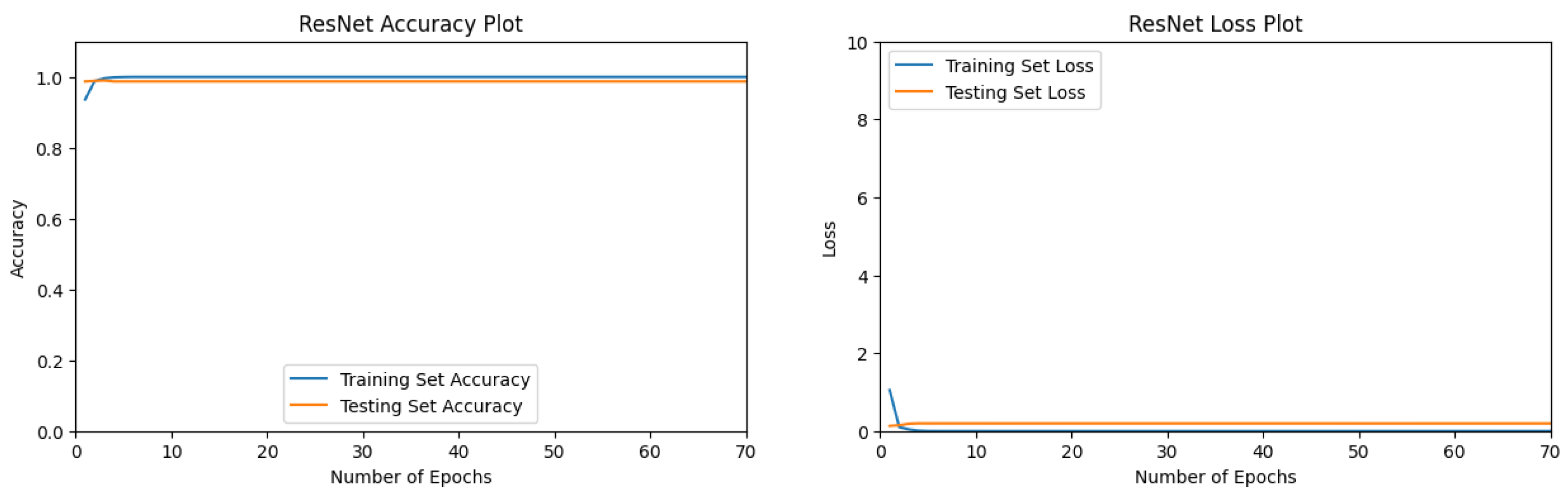
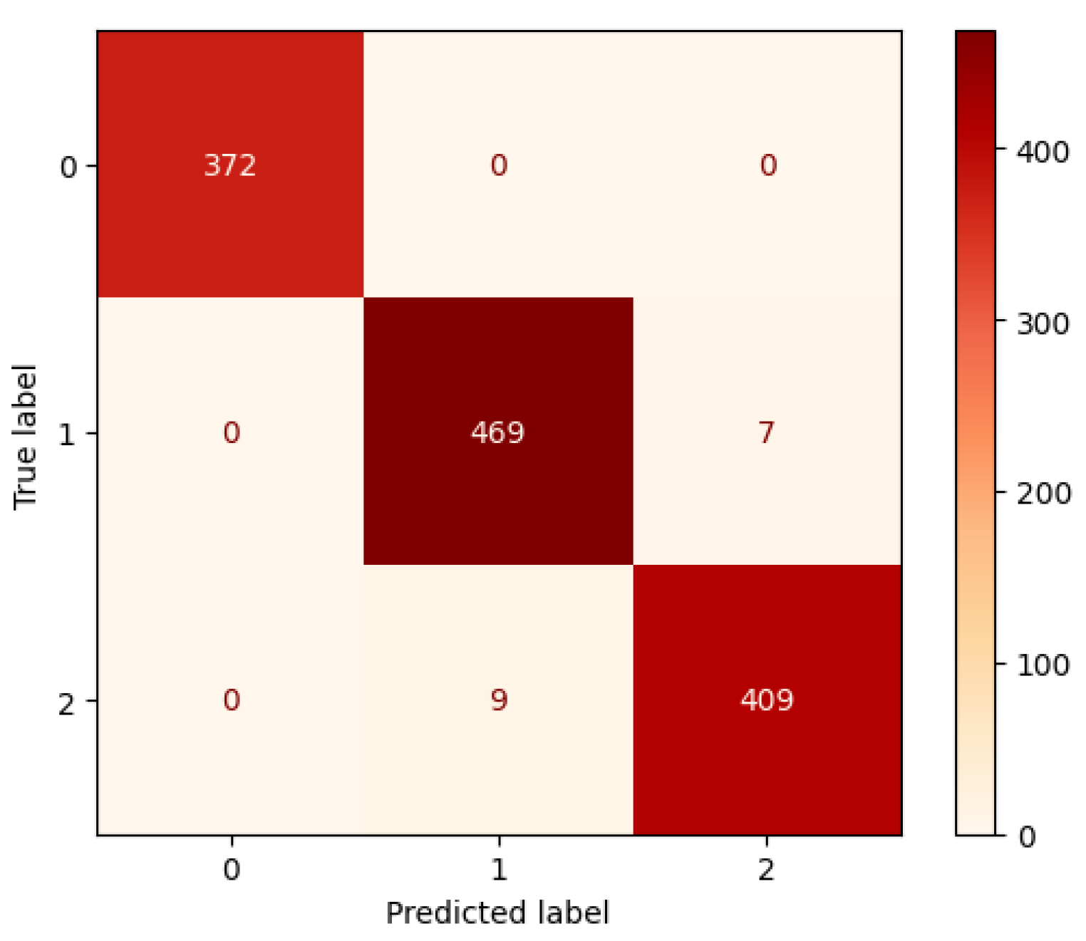
3.1.4. ResNet Performance

Our ResNet50 [55] model reached validations accuracies of near 100%, as demonstrated in Figure 9. The final validation accuracy after 70 epochs was 98.74% on a separate run.

The Desert category, label 0, was predicted accurately upon each actual occurrence and every prediction for the desert category was accurate, well. The confusion matrix in Figure 10 shows the flawless predictions by our ResNet50 [55] model for the Desert category.

Table 5 confirms that the Desert category has a score of 1.0 for precision, recall, and F1-Score by our ResNet50 [55] model. The Neither category received a score of 0.98 for precision, recall, and F1-Score.

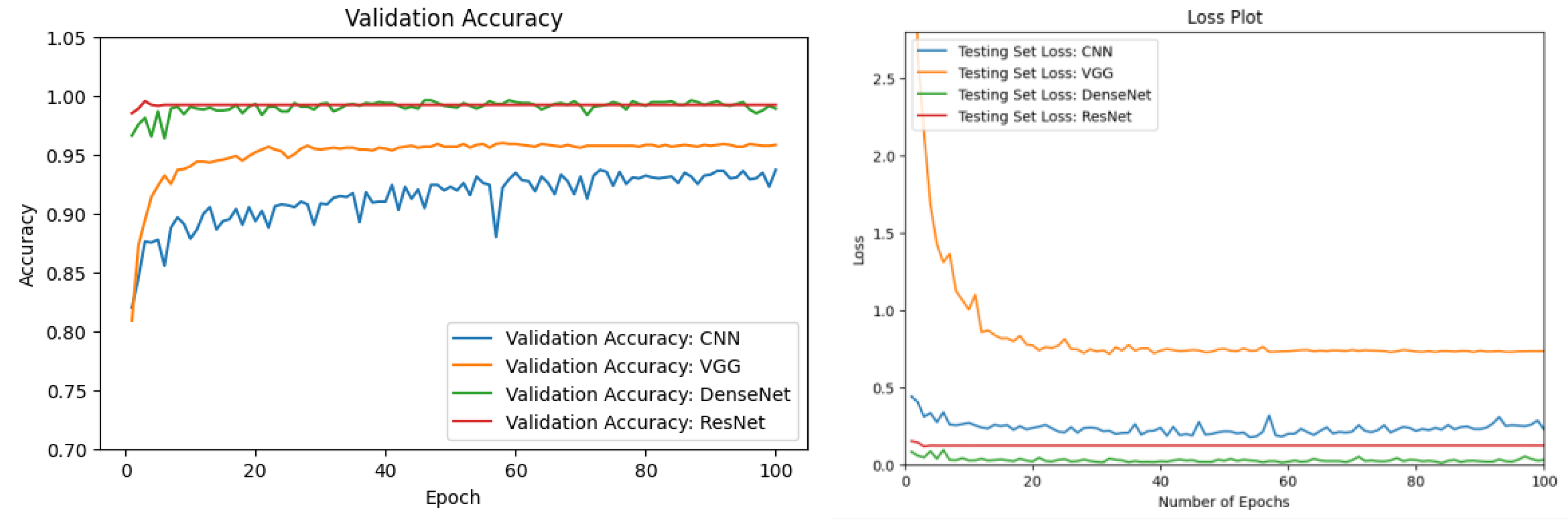
3.2. ML Model Comparison

In this section, we compare and contrast the performance of our 4 ML models for the task of climate change related natural disaster detection. Our ML Python Module was run over 100 epochs with a batch size of 128. The testing accuracies and testing loss can be seen in Figure 11.

After 100 epochs, our ResNet50 [55] model reached a slightly higher validation accuracy of 99.21% than our DenseNet201 [50] Optimized model. As can be seen in Table 6, our DenseNet201 [50] Optimized model reached 98.89% validation accuracy.

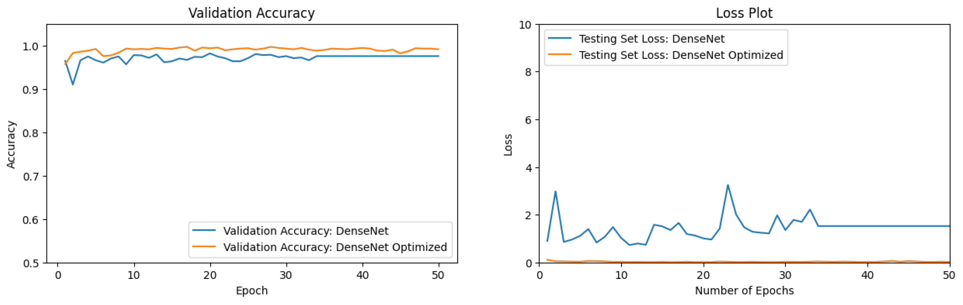
3.3. Optimization of DenseNet

Our DenseNet201 [50] model was chosen for optimization. The DenseNet201 [50] Optimized model contained additional layers such as a Rescaling layer and a Data Augmentation layer. The two ML models, our basic DenseNet201 [50] and our DenseNet201 [50] Optimized were run over 50 epochs with a batch size of 64. The performance of both our basic DenseNet201 [50] model and our DenseNet201 [50] Optimized model can be seen in Figure 12.

According to Table 7, our DenseNet201 [50] Optimized model yielded a higher validation accuracy than our basic DenseNet201 [50] model.

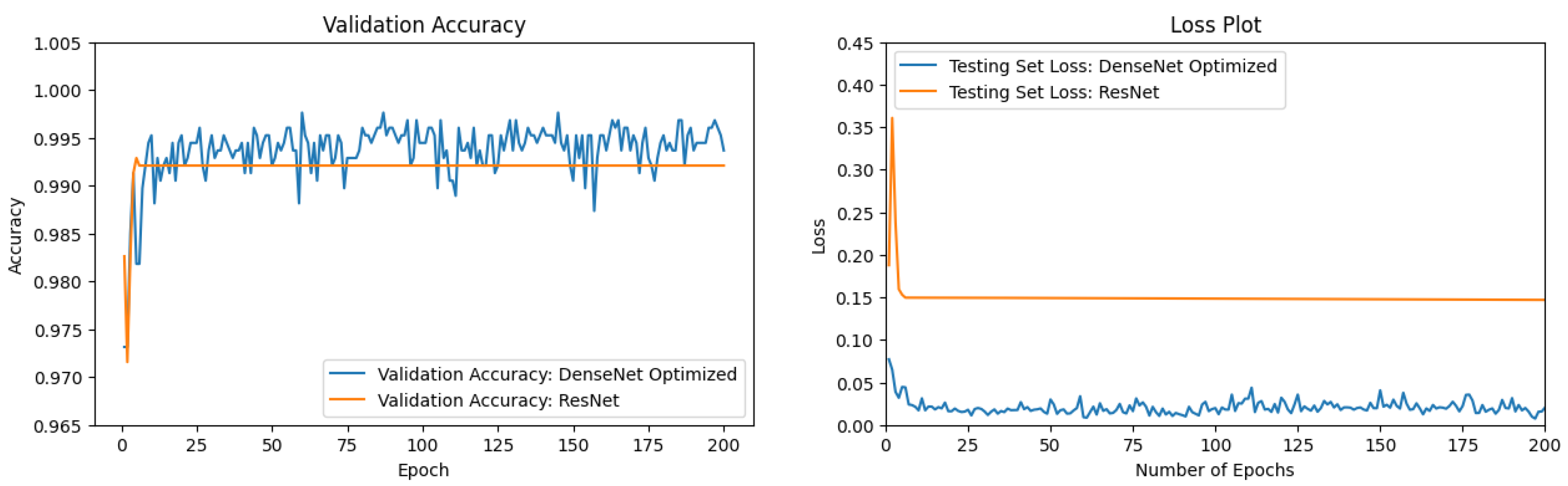
3.4. ResNet vs. DenseNet Optimized

In our previous ML Model Comparison section (3.2), the ResNet50 [55] model and the DenseNet201 [50] Optimized model appeared to perform similarly on the validation accuracy plot. To more clearly visualize their performance, our ResNet50 [55] model was juxtaposed with your DenseNet201 [50] Optimized model for a longer run over more epochs. Our ML Python module was run for 200 epochs with a batchsize of 128. The validation accuracies for our DenseNet201 [50] Optimized model oscillated from approximately 0.987 - 0.998, as can be seen in Figure 13. DenseNet201 [50] Optimized demonstrated a lower testing loss and a consistently higher testing accuracy when run 200 epochs.

As can be seen in Table 8, our DenseNet201 [50] Optimized model reached a validation accuracy of 99.37% after 200 epochs.

4. Discussion

Our compiled Climate Change Dataset provided enough images for our ML models to extract key features in accurately detecting the natural disasters examined in this study. Our 4 ML models all performed well at climate change related natural disaster detection based on images from our Climate Change Dataset. The 4 ML models, VGG16, CNN, DenseNet201 Optimized, and ResNet50 all reached high validation accuracies of 95.81%, 93.68%, 98.89%, and 99.21% respectively over 100 epochs. Our DenseNet201 model was selected for optimization techniques such as data augmentation. Validation accuracy increased from 97.55% to 99.13% when additional layers were added to DenseNet201 for optimization purposes. Testing set loss was lower, as well, with cross-entropy loss dropping from 1.5234 to a much lower cross-entropy loss of 0.0196. Although, all 4 ML models performed well at natural disaster detection, ResNet50 and DenseNet201 Optimized yielded higher validation accuracies and appeared to demonstrate similar performance on the validation accuracy plot (Figure 11). Oluibukun Gbenga Ajayi and John Ashi found that the ML model validation accuracy showed an increasing upward trend as the number of epochs increases until the validation accuracy finally converges [58]. We ran the two ML models over a higher epoch count to compare the two ML models. ResNet50 and DenseNet201 Optimized reached 99.21% and 99.37% respectively over 200 epochs. For ML professionals that prefer validation accuracies in the 90% - 97% range, then our VGG16 and our CNN model would suite their purposes better. Our study highlights the power of AI in addressing some of the most pressing environmental challenges. This study intended to use AI for Climate Change and Environmental Sustainability. We are determined to use AI for the benefit of society, particularly in mitigating the negative effects of climate change.

References

1. B. Clarke, F. Otto, R. Stuart-Smith and L. Harrington, "Extreme weather impacts of climate change: an attribution perspective," Environmental Research: Climate, pp. 1-26. doi:10.1088/2752-5295/ac6e7d, 2022.
2. Intergovernmental_Panel_On_Climate_Change(IPCC), "Climate Change 2021 – The Physical Science Basis: Working Group I Contribution to the Sixth Assessment Report of the Intergovernmental Panel on Climate Change," Cambridge University Press, Cambridge, 2023.
3. C. Raymond, T. Matthews and R. Horton, "The emergence of heat and humidity too severe for human tolerance," Science Advances, vol. 6, no. 19, pp. 1-8. doi: 10.1126/sciadv.aaw1838, 2020.
4. EMDAT, "The emergency events database," (Univ of Louvain - CRED), 2019.
5. C. Cho, R. Li, S.-Y. Wang, J. -H. Yoon and R. R. Gillies, "Anthropogenic Footprint of Climate Change in the June 2013 Northern India Flood," Climate Dynamics, pp. 797-805. doi: 10.1007/s00382-015-2613-2, 2015.
6. P. Pall, C. Patricola, M. Wehner, D. Stone, C. Paciorek and W. Collins, "Diagnosing conditional anthropogenic contributions to heavy Colorado rainfall in September 2013," Weather and Climate Extremes, vol. 17, pp. 1-6. doi:10.1016/j.wace.2017.03.004, 2017.
7. K. van der Wiel, S. B. Kapnick, G. J. van Oldenborgh, K. Whan, S. Philip, G. Vecchi, R. K. Singh, J. Arrighi and H. Cullen, "Rapid attribution of the August 2016 flood-inducing extreme precipitation in south Louisiana to climate change," Hydrology and Earth System Sciences, vol. 21, no. 2, pp. 897-921. doi:10.5194/hess-21-897-2017, 2017.
8. S. Philip, S. F. Kew, G. J. van Oldenborgh, E. Aalbers, R. Vautard, F. Otto, K. Haustein, F. Habets and R. Singh, "Validation of a rapid attribution of the May/June 2016 flood-inducing precipiation in France to climate change," Journal of Hydrometerorology, vol. 19, no. 11, pp. 1881-1898. doi: 10.1175/JHM-D-18-0074.1, 2018.
9. B. Teufel, L. Sushama, O. Huziy, G. T. Diro, D. Jeong, K. Winger, C. Garnaud, R. de Elia, F. W. Zwiers, H. D. Matthews and V.-T.-V. Nguyen, "Investigation of the mechanisms leading to the 2017 Montreal flood," Climate Dynamics, pp. 4193-4206. doi: 10.1007/s00382-018-4375-0, 2019.
10. J. Huang, G. Zhang, Y. Zhang, X. Guan, Y. Wei and R. Guo, "Global desertification vulnerability to climate change and human activities," Land Degrad Dev., pp. 1380-1391. doi: 10.1002/ldr.3556, 2020.
11. UNCCD, "United Nations convention to combat desertification in countries experiencing serous drought and/or desertification, paticularly in Africa," Paris, 1994.
12. S. Nicholson, C. Tucker and M. Ba, "Desertification, Drought, and Surface Vegetation: An Example from the West African Sahel," Bulletin of the American Meteorological Society, vol. 79, pp. 815-829. doi: 10.1175/1520-0477(1998)079<0815:DDASVA>2.0.CO;2, 1998.
13. M. Sivakumar, "Interactions between climate and desertification," Agricultural and Forest Meteorology, vol. 142, no. 2-4, pp. 143-155. doi: 10.1016/j.agrformet.2006.03.025, 2007.
14. MillenniumEcosystemAssessment(MEA), "Ecosystems and human well-being: Desertification synthesis.," Washington, D.C.: World Resources Institute, 2005.
15. D. Hernández, J.-C. Cano, F. Silla, C. T. Calafate and J. M. Cecilia, "AI-Enabled Autonomous Drones for Fast Climate Change Crisis Assessment," IEEE Internet of Things Journal, pp. 7286-7297. doi: 10.1109/JIOT.2021.3098379, 2022.
16. Alsumayt, N. El-Haggar, L. Amouri, Z. M. Alfawaer and S. S. Aljameel, "Smart Flood Detection with AI and Blockchain Integration in Saudi Arabia Using Drones," Sensors, pp. 1-30. https://doi.org/ 10.3390/s23115148, 2023.
17. N. S. Intizhami, E. Q. Nuranti and N. I. Bahar, "Dataset for flood area recognition with semantic segmentation," Data in Brief, vol. 51, pp. 1-7. https://doi.org/10.1016/j.dib.2023.109768, 2023.
18. F. S. Alrayes, S. S. Alotaibi, K. A. Alissa, M. Maashi, A. Alhogail, N. Alotaibi, H. Mohsen and A. Motwakel, "Artificial Intelligence-Based Secure Communication and Classification for Drone-Enabled Emergency Monitoring Systems," Drones, vol. 6, no. 9, pp. 1-18. https://doi.org/10.3390/drones6090222, 2022.
19. R. Karanjit, R. Pally and S. Samadi, "FloodIMG: Flood image DataBase system," Data in Brief, vol. 48, pp. 1-13. https://doi.org/10.1016/j.dib.2023.109164, 2023.
20. D. Hamlington, A. Tripathi, D. R. Rounce, M. Weathers, K. H. Adams, C. Blackwood, J. Carter, R. C. Collini, L. Engeman, M. Haasnoot and R. E. Kopp, "Satellite monitoring for coastal dynamic adaptation policy pathways," Climate Risk Management, vol. 42, pp. 1-16. https://doi.org/10.1016/j.crm.2023.100555, 2023.
21. J. P. Dash, G. D. Pearse and M. S. Watt, "UAV Multispectral Imagery Can Complement Satellite Data for Monitoring Forest Health," Remote Sens., pp. 1-22. https://doi.org/10.3390/rs10081216, 2018.
22. K. Dilmurat, V. Sagan and S. Moose, "AI-DRIVEN MAIZE YIELD FORECASTING USING UNMANNED AERIAL VEHICLE-BASED HYPERSPECTRAL AND LIDAR DATA FUSION," ISPRS Annals of the Photogrammetry, Remote Sensing and Spatial Information Sciences, pp. 193-198. https://doi.org/10.5194/isprs-annals-V-3-2022-193-2022, 2022.
23. Raniga, N. Amarasingam, J. Sandino, A. Doshi, J. Barthelemy, K. Randall, S. A. Robinson, F. Gonzalez and B. Bollard, "Monitoring of Antarctica’s Fragile Vegetation Using Drone-Based Remote Sensing, Multispectral Imagery and AI," Sensors, pp. 1-29. https://doi.org/10.3390/s24041063, 2024.
24. A. Santangeli, Y. Chen, E. Kluen, R. Chirumamilla, J. Tiainen and J. Loehr, "Integrating drone-borne thermal imaging with artificial intelligence to locate bird nests on agricultural land," Scientific Reports, pp. 1-8. https://doi.org/10.1038/s41598-020-67898-3, 2020.
25. H. R. G. Malamiri, F. A. Aliabad, S. Shojaei, M. Morad and S. S. Band, "A study on the use of UAV images to improve the separation accuracy of agricultural land areas," Computers and Electronics in Agriculture, vol. 184, pp. 1-13. https://doi.org/10.1016/j.compag.2021.106079, 2021.
26. Alvarez-Vanhard, T. Corpetti and T. Houet, "UAV & satellite synergies for optical remote sensing applications: A literature review," Science of Remote Sensing, vol. 3, pp. 1-16. https://doi.org/10.1016/j.srs.2021.100019, 2021.
27. A. Marx, D. McFarlane and A. Alzahrani, "UAV data for multi-temporal Landsat analysis of historic reforestation: a case study in Costa Rica," International Journal of Remote Sensing, pp. 2331-2348. doi:10.1080/01431161.2017.1280637, 2017.
28. N. Hassan, A. S. Musa Miah and J. Shin, "Residual-Based Multi-Stage Deep Learning Framework for Computer-Aided Alzheimer’s Disease Detection," Journal of Imaging, vol. 10, no. 6, pp. 1-21. doi:10.3390/jimaging10060141, 2024.
29. A.M. Ibrahim, M. Elbasheir, S. Badawi, A. Mohammed and A. F. M. Alalmin, "Skin Cancer Classification Using Transfer Learning by VGG16 Architecture (Case Study on Kaggle Dataset)," Journal of Intelligent Learning Systems and Applications, vol. 15, pp. 67-75. doi: 10.4236/jilsa.2023.153005, 2023.
30. B. Abu Sultan and S. S. Abu-Naser, "Predictive Modeling of Breast Cancer Diagnosis Using Neural Networks:A Kaggle Dataset Analysis," International Journal of Academic Engineering Research, pp. 1-9, 2023.
31. S. Bojer and J. P. Meldgaard, "Kaggle forecasting competitions: An overlooked learning opportunity," International Journal of Forecasting, vol. 37, no. 2, pp. 587-603. doi:10.1016/j.ijforecast.2020.07.007, 2021.
32. J. Ker, L. Wang, J. Rao and T. Lim, "Deep Learning Applications in Medical Image Analysis," IEEE Access, pp. 9375-9389. doi: 10.1109/ACCESS.2017.2788044, 2018.
33. R. Ghnemat, S. Alodibat and Q. A. Al-Haija, "Explainable Artificial Intelligence (XAI) for Deep Learning Based Medical Imaging Classification," Journal of Imaging, pp. 1-31. doi:10.3390/jimaging9090177, 2023.
34. Kwenda, M. Gwetu and J. V. Fonou-Dombeu, "Hybridizing Deep Neural Networks and Machine Learning Models for Aerial Satellite Forest Image Segmentation," Journal of Imaging, pp. 1-34. doi: 10.3390/jimaging10060132 PMCID: PMC11204628 , 2024.
35. T. Boston, A. Van Dijk and R. Thackway, "U-Net Convolutional Neural Network for Mapping Natural Vegetation and Forest Types from Landsat Imagery in Southeastern Australia," Journal of Imaging, pp. 1-24. doi:10.3390/jimaging10060143, 2024.
36. A. Kumar, A. Jaiswal, S. Garg, S. Verma and S. Kumar, "Sentiment Analysis Using Cuckoo Search for Optimized Feature Selection on Kaggle Tweets," International Journal of Information Retrieval Research , vol. 9, no. 1, pp. 1-15. doi: 10.4018/IJIRR.2019010101, 2019.
37. Albin Ahmed, A. Shaahid, F. Alnasser, S. Alfaddagh, S. Binagag and D. Alqahtani, "Android Ransomware Detection Using Supervised Machine Learning Techniques Based on Traffic Analysis," Sensors, pp. 1-21. doi:10.3390/s24010189, 2024.
38. S. B. Taieb and R. J. Hyndman, "A gradient boosting approach to the Kaggle load forecasting competition," International Journal of Forecasting, vol. 30, no. 2, pp. 382-394. doi: 10.1016/j.ijforecast.2013.07.005, 2014.
39. "Kaggle," [Online]. Available: https://www.kaggle.com/. [Accessed 1 10 2024].
40. RahulTP, "Louisiana flood 2016," Kaggle, [Online]. Available: www.kaggle.com/datasets/rahultp97/louisiana-flood-2016. [Accessed 1 Oct 2024].
41. M. Wang, "FDL_UAV_flooded areas," Kaggle, [Online]. Available: www.kaggle.com/datasets/a1996tomousyang/fdl-uav-flooded-areas. [Accessed 1 Oct 2024].
42. R. Rupak, "Cyclone, Wildfire, Flood, Earthquake Database," Kaggle, [Online]. Available: www.kaggle.com/datasets/rupakroy/cyclone-wildfire-flood-earthquake-database. [Accessed 1 Oct 2024].
43. M. Reda, "Satellite Image Classification," Kaggle, [Online]. Available: www.kaggle.com/datasets/mahmoudreda55/satellite-image-classification. [Accessed 1 Oct 2024].
44. G. Mystriotis, "Disasters Dataset," Kaggle, [Online]. Available: https://www.kaggle.com/datasets/georgemystriotis/disasters-dataset. [Accessed 1 Oct 2024].
45. A. Bhardwaj and Y. Tuteja, "Aerial Landscape Images," Kaggle, [Online]. Available: https://www.kaggle.com/datasets/ankit1743/skyview-an-aerial-landscape-dataset. [Accessed 1 Oct 2024].
46. Y. Tuteja and A. Bhardwaj, "Aerial Images of Cities," Kaggle, [Online]. Available: https://www.kaggle.com/datasets/yessicatuteja/skycity-the-city-landscape-dataset. [Accessed 1 Oct 2024].
47. Demir, K. Koperski, D. Lindenbaum, G. Pang, J. Huang and S. Basu, "DeepGlobe 2018: A Challenge to Parse the Earth through Satellite Images," in 2018 IEEE/CVF Conference on Computer Vision and Pattern Recognition Workshops (CVPRW), Salt Lake City, UT, 2018.
48. Simonyan and A. Zisserman, "Very Deep Convolutional Networks for Large-Scale Image Recognition," arXiv, pp. 1-14. doi:10.48550/arXiv.1409.1556, 2015.
49. X. Zan, X. Zhang, Z. Xing, W. Liu, X. Zhang, W. Su, Z. Liu, Y. Zhao and S. Li, "Automatic Detection of Maize Tassels from UAV Images by Combining Random Forest Classifier and VGG16," Remote Sensing, vol. 12, no. 18, pp. 1-17. doi : 10.3390/rs12183049, 2020.
50. G. Huang, Z. Liu, L. van der Maaten and K. Q. Weinberger, "Densely Connected Convolutional Networks," arXiv, pp. 1-8. doi:10.48550/arXiv.1608.06993, 2018.
51. A. Mumumi and F. Mumuni, "Data augmentation: A comprehensive survey of modern approaches," Array, vol. 16, pp. 1-27. doi : 10.1016/j.array.2022.100258, 2022.
52. X. Pei, Y. h. Zhao, L. Chen, Q. Guo, Z. Duan, Y. Pan and H. Hou, "Robustness of machine learning to color, size change, normalization, and image enhancement on micrograph datasets with large sample differences," Materials & Design, vol. 232, pp. 1 - 13. doi : 10.1016/j.matdes.2023.112086, 2023.
53. G. Habib and S. Qureshi, "GAPCNN with HyPar: Global Average Pooling convolutional neural network with novel NNLU activation function and HYBRID parallelism," Frontiers in Computational Neuroscience, vol. 16, pp. 1 - 18. doi : 10.3389/fncom.2022.1004988, 2022.
54. S. Shabbeer Basha, S. R. Dubey, V. Pulabaigari and S. Mukherjee, "Impact of fully connected layers on performance of convolutional neural networks for image classification," Neurocomputing, vol. 378, pp. 112-119. doi: 10.1016/j.neucom.2019.10.008, 2020.
55. He, X. Zhang, S. Ren and J. Sun, "Deep Residual Learning for Image Recognition," arXiv, pp. 1 - 12. doi:10.48550/arXiv.1512.03385, 2015.
56. W. Alsabhan and T. Alotaiby, "Automatic Building Extraction on Satellite Images Using Unet and ResNet50," Computational Intelligence and Neuroscience, pp. 1-12. doi : 10.1155/2022/5008854, 2022.
57. A. Zafar, M. Aamir, N. M. Nawi, A. Arshad, S. Riaz, A. Alruban, A. K. Dutta and S. Almotairi, "A Comparison of Pooling Methods for Convolutional Neural Networks," Applied Sciences, vol. 12, no. 17, pp. 1-21. doi : 10.3390/app12178643, 2022.
58. A.G. Ajayi and J. Ashi, "Effect of varying training epochs of a Faster Region-Based Convolutional Neural Network on the Accuracy of an Automatic Weed Classification Scheme," Smart Agricultural Technology, vol. 3, pp. 1-14. doi: 10.1016/j.atech.2022.100128, 2023.
Figure 1. These are example images from the Climate Change Dataset. The example images on top show an example image from the Flood and Desert category. On the bottom row, the example images show the corresponding example image from the neither category.
Preprints 145022 g001
Figure 2. Transfer Learning Framework.
Preprints 145022 g002
Figure 3. The left figure shows the accuracy curve for our VGG16 model. The right figure shows the loss curve for our VGG16 model.
Preprints 145022 g003
Figure 4. Confusion matrix for VGG16 after 70 epochs.
Preprints 145022 g004
Figure 5. The left figure shows the accuracy curve for our DenseNet201 Optimized model. The right figure shows the loss curve for our DenseNet201 Optimized model.
Preprints 145022 g005
Figure 6. DenseNet201 Optimized model after 70 epochs.
Preprints 145022 g006
Figure 7. The left figure shows the accuracy curve for our CNN model. The right figure shows the loss curve for our CNN model.
Preprints 145022 g007
Figure 8. Confusion matrix for our CNN model after 70 epochs.
Preprints 145022 g008
Figure 9. The left figure shows the accuracy curve for our ResNet50 model. The right figure shows the loss curve for our ResNet50 model.
Preprints 145022 g009
Figure 10. Confusion matrix for our ResNet50 model after 70 epochs.
Preprints 145022 g010
Figure 11. The left figure shows the accuracy curve for all 4 of our ML models (CNN, VGG16, DenseNet201 Optimized, ResNet50). The right figure shows the loss curve for all 4 ML models.
Preprints 145022 g011
Figure 12. The left figure shows the accuracy curve for our basic DenseNet201 model vs. our DenseNet201 Optimized model. The right figure shows the loss curve for our basic DenseNet201 model vs. our DenseNet201 Optimized model.
Preprints 145022 g012
Figure 13. The left figure shows the accuracy curve for our DenseNet201 Optimized model vs. our ResNet50 model. The right figure shows the loss curve for our DenseNet201 Optimized model vs. our ResNet50 model.
Preprints 145022 g013