
Submitted:
03 January 2025
Posted:
03 January 2025
You are already at the latest version
Abstract
This study explores how the variation of atmospheric gravity waves (AGWs) get modified and intensified during tropical cyclones using high-resolution ERA5 reanalysis data. AGWs play a vital role in understanding tropical cyclone dynamics due to their connection with energy and momentum transfer in the atmosphere. Different issues related to six tropical cyclones in the Bay of Bengal from 2019 to 2022, spanning different intensities and seasonal conditions, have been analyzed. Using temperature and pressure data across 37 vertical levels, several variables like perturbation temperature and potential energy Ep profiles associated with AGWs are computed. Spatial temperature distributions and Ep exhibit spiral formations resembling cyclone structures with significant altitude-dependent variations. Temperature signatures are observed at altitudes between 1.5 km and 5.5 km, varying by season and intensity, while Ep signatures were prominent between 14.55 km and 19.31 km, peaking at 15.79 km for most cyclones except Cyclone Fani, which peaked at 17.66 km. Ep values ranged from 10 to 25 J/kg, reflecting strong AGW-cyclone interactions. These findings highlight the influence of cyclone intensity, seasonality, and atmospheric dynamics on AGW behaviour, enhancing the understanding of energy transfer processes in the upper troposphere and lower stratosphere.
Keywords:
Tropical Cyclone
; Atmospheric Dynamics
; ECMWF and ERA5
; Atmospheric Temperature Gradient
; Atmospheric Gravity Wave
1. Introduction
In several important works, strong evidence shows an increase in the intensity and frequency of tropical cyclones, particularly in regions like the Indian Ocean, in the last two decades due to increasing sea surface temperatures and changing atmospheric conditions associated with global climate change [1,2]. The destructive potential of these cyclones makes policymakers think of the importance of accurate forecasting and climate adaptation strategies in coastal regions. When warm and moist air ascends rapidly in the cyclone’s eyewall and rainbands, latent heat is released, destabilizing the surrounding atmosphere. This release of latent heat drives updrafts that push air parcels upwards, creating a buoyancy imbalance. Atmospheric gravity waves (AGWs) are oscillations in the atmosphere where buoyancy acts as the restoring force. These waves can transport energy away from the cyclone, helping to redistribute heat and momentum in the atmosphere around the storm [3,4]. In tropical cyclones, AGW generation is closely tied to the dynamics of the eyewall, where the most intense convection occurs. As convective cells within the eyewall undergo rapid vertical motion, they displace surrounding air, causing pressure and density perturbations. These disturbances can propagate as gravity waves, which carry momentum and energy away from the convective core [5]. Gravity waves from these regions can be powerful because the cyclonic environment provides a continuous source of buoyant energy, particularly in storms with a warm core. This continued energy supply allows for sustained AGW formation and propagation, influencing areas far beyond the immediate vicinity of the storm. The vertical and horizontal wind shear commonly present in and around tropical cyclones can also trigger gravity waves. Tropical cyclones are known for creating localized regions of strong wind shear due to the differential flow around the storm center. This shear results in imbalances that displace air parcels vertically, leading to oscillations as gravity attempts to restore equilibrium. Gravity waves formed by this mechanism are often lower in frequency but can be long-lived and carry energy far from the storm. These interactions can contribute to turbulence and affect the upper and lower stratosphere’s momentum distribution[6].
AGWs can have significant impacts on the cyclone itself, as well as on the surrounding atmosphere. When AGWs propagate outward, they interact with various atmospheric layers, potentially affecting the storm’s structure and intensity. For example, gravity waves generated by convection in the eyewall can modulate angular momentum distribution in the cyclone, impacting wind speed and storm symmetry [7,8]. Additionally, AGWs are prone to influence the upper atmosphere by redistributing heat and moisture, which can modify the environmental conditions in ways that may either intensify or weaken the storm. Studying these wave-induced dynamics is crucial for understanding cyclone behavior, as AGWs represent an intricate pathway for energy transfer and contribute to complex feedback mechanisms that affect storm evolution.
Studies on gravity wave activities have highlighted their significant role in atmospheric dynamics and vertical coupling. [9] provided observational evidence of gravity waves generated by convection and their coupling effects in the mesosphere-lower thermosphere (MLT) region over tropical areas. Comprehensive research have been carried out focussing the hydration and convection processes during the cyclonic storm by [10,11,12]. [13] investigated the dominant sources of gravity waves during the Indian summer monsoon using ground-based measurements, emphasizing the role of convective processes. Furthermore, [14] analyzed gravity wave activities during stratospheric sudden warming events using SOFIE temperature data, underscoring their impact on stratospheric and mesospheric dynamics. A lot of studies revealed such excitation of AGW as computed from multiple instruments starting from MST Radar and GPS Radio Occultation (RO) and satellite observations. [15] explored the contribution of gravity waves to tropical convection using the Indian MST radar, revealing their influence in the upper troposphere and lower stratosphere. Significant studies using RO have been reported for many cyclones and typhoons by [16,17,18,19,20,21,22]. [23] reported a study on AGW generated by Typhoon Ewiniar using satellite observations and numerical simulation.
In recent years, the Bay of Bengal region has been frequently impacted by several significant tropical cyclones, notably Cyclones Fani (2019), Bulbul (2019), Amphan (2020), Yass (2021), Gulab (2021), and Asani (2022). Cyclone Fani, an extremely severe cyclone, made landfall in Odisha, India, causing extensive structural damage, flooding, and power outages due to intense winds and heavy rainfall. Later, in 2019, Cyclone Bulbul struck West Bengal and Bangladesh as a severe cyclonic storm, resulting in widespread flooding and infrastructure damage. The 2020 Cyclone Amphan, one of the most intense cyclones recorded in the region in recent decades, led to devastating impacts in West Bengal and Bangladesh, with severe damages by tremendous wind speed, coastal flooding, and significant displacement of communities. Cyclone Yass in 2021 primarily impacted the eastern coastal regions of Odisha and West Bengal, causing flooding and heavy precipitation. Cyclone Gulab also emerged in 2021, affecting eastern India, and its remnants later moved into the Arabian Sea and re-intensified as Cyclone Shaheen. In 2022, Cyclone Asani, although less intense, influenced the coastal areas of Andhra Pradesh with significant rainfall before dissipating over the Bay of Bengal without direct landfall. These recent cyclones represent a pattern of increasing frequency and intensity of tropical storms in the Indian Ocean, potentially linked to climate variability and warming ocean temperatures, underscoring the need for enhanced cyclone preparedness and adaptive strategies in cyclone-prone coastal regions.
In the present manuscript, we have investigated and tried to estimate the degree of intensification of atmospheric gravity wave (AGW) energy during multiple tropical cyclones, utilizing high-resolution ERA5 reanalysis data. By analyzing wave energy patterns and dynamics across various cyclonic events, we identify specific conditions under which AGW energy intensifies, such as extreme convective activity, wind shear, and rapid changes in pressure fields within the cyclone environment. ERA5’s high temporal as well as spatial resolution allows us to observe subtle impaction in the variations in wave propagation and energy distribution. This attempt enables a comprehensive examination of the mechanisms behind the enhancement of AGW under extreme atmospheric conditions. Our findings provide new insights into the role of tropical cyclones in modulating AGW energy, advancing the understanding of cyclone-induced atmospheric wave phenomena and their implications for energy and momentum transfer within the upper troposphere and lower stratosphere.
2. Data and Analysis
We have taken all six cyclones from 2019 to 2022 into consideration, which made landfall at the coast of the Bay of Bengal in the Indian state boundary. We collect detailed information on these cycones from the database of the Indian Mateorological Department (IMD) (https://mausam.imd.gov.in). Among them, two (Gulab in winter and Asani in summer) are severe cyclones, two (Bulbul in winter and Yaas in summer) are very severe cyclones, one (Fani in summer) is an extremely severe cyclone, and one (Amphan in summer) is a super cyclone. The details of cyclones, their landfall date and position, and the severity details are given in Table 1.
Figure 1 shows the spatio-temporal trajectory of the six cyclones. This study employed ArcGIS Pro to generate cyclone tracks using the extensive ERA5 Hourly data on pressure levels from 1940 to the present. The analysis concentrated on individual cyclones, tracking them from inception to dissipation. The accompanying legends meticulously documented each cyclone’s lifespan. Within Arc GIS and ArcGIS Pro, the visualization of the ERA5 data enabled the identification and placement of tracking points at the center of each cyclone’s eye, representing its daily position. These tracking points were then used to create vector datasets representing the cyclone tracks. The accuracy of these generated tracks, a thorough validation process was conducted. The cyclone tracks derived from ERA5 data were compared with the authoritative dataset from the India Meteorological Department (IMD). The validation results demonstrated a high level of agreement, with an impressive 85% accuracy.
The European Centre for Medium-Range Weather Forecasts (ECMWF) is one of the world’s leading centers for global weather prediction, offering high-resolution numerical weather data and reanalysis products. Among these products, the ECMWF Reanalysis 5th Generation, known as ERA5, is a high-quality atmospheric reanalysis dataset that provides hourly data on a wide array of atmospheric, oceanic, and land-surface variables from 1950 to the present (https://www.ecmwf.int/en/forecasts/dataset/ecmwf-reanalysis-v5). ERA5 combines observational data with ECMWF’s forecasting models using data assimilation techniques, resulting in a spatially and temporally consistent dataset. This makes ERA5 particularly valuable for studying various atmospheric processes, including the formation and propagation of atmospheric gravity waves (AGWs), which are influenced by a range of meteorological parameters such as wind speed, temperature, and pressure [24].
In the study of AGWs, ERA5 is especially useful due to its high spatial and temporal resolution, allowing researchers to capture the fine-scale features of these waves. AGWs often emerge from localized atmospheric disturbances, such as those generated within intense convective regions of cyclonic storms. To accurately capture the dynamics of AGW generation, it is essential to have data that reflect both the large-scale and mesoscale atmospheric conditions. ERA5’s re-analysis provides a comprehensive view of these conditions, offering insights into the thermodynamic and kinematic structures contributing to AGW formation. This data can be used to identify and analyze the conditions conducive to gravity wave generation, such as strong wind shear, high levels of atmospheric instability, or intense convection within the storm’s core [25]. By examining the pressure, temperature, and wind patterns recorded in ERA5, researchers can study how AGWs transport energy and momentum across the troposphere and stratosphere, influencing larger atmospheric circulation patterns. For instance, the vertical and horizontal propagation of AGWs generated by tropical cyclones can be traced in ERA5, allowing for a detailed analysis of how these waves interact with the surrounding atmosphere and modify weather patterns in regions far from their source. This capability has been utilized in numerous studies to understand the role of AGWs in modulating cyclone dynamics and their potential influence on stratospheric processes and even global climate phenomena [26].
The altitude profiles of the temperature data for the six selected cyclones are taken from the ERA5 re-analysis database. We collected re-analysis data for temperature readings at 37 discrete pressure levels, ranging from 1000 hPa (at a height of 110 meters above sea level) to 1 hPa (at a height of 32.43 km). Data are collected for three consecutive days (before the landfall, during landfall, and after the landfall) at one-hour interval for each cyclone. Python is used as the primary tool for data analysis. We first separate four specific time instants to investigate the temperature profiles. The times are (a) 24 hours and (b) 12 hours before the landfall, (c) at the time of the landfall, and (d) 6 hours after the landfall. Each data set contains four columns: (i) latitude, (ii) longitude, (iii) pressure levels, and (iv) corresponding temperatures. For all cyclones, we take the data within the area bounded by N to N and E to E. The altitude () profile, corresponding to the different pressure levels (), is computed using the following formula taken from (SOURCE):
A grid dataset is computed by rearranging the data by descending-order latitudes and ascending-order longitudes, including the computed altitude profile. Then, the logarithm of the temperature is calculated, and the logarithmic profile is fitted with a third-order polynomial using the altitudes (z). The difference between the logarithmic temperature and the fitted polynomial is calculated. A 4 km boxcar filter is applied to eliminate all the wavelengths less than 4 km. We add the filtered residual values and the fitted temperatures to compute the final profile. The antilogarithm of the final profile is the least square fit (LSF). We use these LSFs, ranging from 1 to 5, to compute the normal zonal mean temperature and other zonal wave components. The background temperature () is the sum of all wave components between 0 and 5. The perturbation temperature () is calculated by subtracting from the original raw temperature data.
The Brunt-Väisälä Frequency (N), which represents the frequency of oscillation of an air parcel in a stable atmosphere, is calculated using,
Here, z = altitude (in km), = specific heat at constant pressure = 1.005 kJ/kg-K, = background temperature, and g = acceleration due to gravity = 0.0098 km/s2. The potential energy () associated with AGW is computed as,
The computation of AGW for altitude profiles of temperature has been validated numerous times using ERA5 and SABER/TIMED instruments during seismic events. Seismogenic impression of AGW has been computed with this methods and reported by [27,28,29,30,31,32,33]. To identify the impact of the AGW due to the abovementioned cyclones, we check the spatial distribution temperature for each pressure level. These distributions follow the conventional spiral formations resembling the cyclonic structure. The intensity of such structural formation is found to be varied with altitude, depending on the cyclone’s severity. We examine the spatial distributions of for each pressure level. Prominent signatures are observed at 50, 70, 100, and 125 hPa pressure levels, following similar spiral formations. Below 14.55 km, values are almost negligible. The variation of at different altitudes as a function of latitude and longitude is also investigated for each cyclone at four-time instants, up to an altitude of 25 km. This range is selected as the most significant variation in for AGWs observed within this altitude. The details of the findings are given in the next section.
3. Results
We choose the following four-time instants to see the spatial-temporal variabilities of the temperature and AGW: 24 hours before landfall (t-24), 12 hours before landfall (t-12), at the time of landfall (t), and 6 hours after landfall (t+6). Figure 2 shows the Spatio-temporal temperature profiles for Cyclone Amphan at an altitude of 1.95 km during its progression. Panels (a), (b), (c), and (d) represent temperature distributions at 12:00 UTC on 19 May 2020, 00:00 UTC on 20 May 2020, 12:00 UTC on 20 May 2020, and 18:00 UTC on 20 May 2020, respectively. The observed spatial variation in temperature and potential energy displays a spiral structure, resembling the characteristic formation of a tropical cyclone. This pattern provides a strong visual evidence of the thermodynamic and dynamic processes involved in cyclone formation.
The temperature signatures of cyclones are observed across different altitudes, ranging from 1.5 km to 5.5 km, with intensity varying across these levels. The most distinct temperature signature for each cyclone is chosen as the representative case. In contrast, the signature of the intensification of AGW potential energy of the cyclones is consistently identified at higher altitudes, specifically between 14.55 km and 19.31 km. The optimal signature for most cyclones occurs at 15.79 km, except for Cyclone Fani, where the best signature is observed at 17.66 km. Cyclone Amphan is chosen as the standard case. For this cyclone, the signature is analyzed at four heights: 14.55 km, 15.79 km, 17.66 km, and 19.31 km, for four selected time samples (Figure 3). The time of landfall for Amphan was at 12 UTC on 20 May 2020, with the best temperature variability signature observed at 1.95 km for the four observation times. For the other five cyclones, only the optimal cases at the time of landfall are presented in Figure 4.
Observational analysis indicates that the potential energy varies between 10 and 25 J/kg during cyclones, with the optimal values typically observed at a height of 14.55 km for all cyclones except Fani, for which the best signature is found at 17.55 km (Figure 4). The analysis also highlights that the optimal temperature profiles for cyclones occur at lower altitudes during winter events. For instance, the best temperature profiles for Cyclone Gulab and Cyclone Bulbul are observed at 2.20 km, and 2.47 km, respectively. In contrast, for summer cyclones of a similar type, as classified by the India Meteorological Department (IMD), the optimal temperature profiles were identified at higher altitudes, typically over 1 km above the winter cases. For example, Cyclone Yaas exhibits its best temperature profile at a height of 3.01 km, while Cyclone Asani at 3.59 km.
So far as the optimal temperature profiles are concerned, a consistent pattern in the altitude of the optimal temperature profiles is obtained from the observational analysis. However, Cyclone Fani is the exception in this case. The best temperature profile is generally observed at lower altitudes for more severe cyclones. For instance, the super cyclone Amphan exhibits its optimal temperature profile at a height of 1.95 km, the very severe cyclone Yaas at 3.01 km, and the severe cyclone Asani at 3.59 km. Notably, all these cyclones occurred during the summer. Cyclone Fani, also a summer cyclone, is classified as an extremely severe cyclone. The India Meteorological Department (IMD) scale rates it as less intense than Amphan but more intense than Yaas. Based on this established pattern, Fani’s best temperature profile was expected to occur between 1.95 km and 3.01 km. However, its optimal temperature profile is observed at a much higher altitude of 4.20 km. For all other cyclones, the most significant profiles are consistently found at a height of 15.79 km. In contrast, for Cyclone Fani, the optimal profile was identified at a significantly higher altitude of 17.66 km.
Figure 5, Figure 6, Figure 7, Figure 8, Figure 9 and Figure 10 depict the latitudinal and longitudinal variation of AGW potential energy during Cyclone Fani, Bulbul, Amphan, Yass, Gulab, and Asani, respectively. Panels (a–d) represent the latitudinal cross-section, while panels (e–h) show the longitudinal cross-section. This representation gives a much clearer view of the directional and altitudinal dependency of the AGW excitation, as presented in Figure 3 and Figure 4. The AGW intensification, a function of latitude, shows a much more prominent signature than longitude as all the cyclones move from south to north latitudes. The intense AGW profile gets depleted for all the cyclones at the landfall time. During landfall, this depletion of Atmospheric Gravity Waves (AGW) occurs due to increased surface friction, reduced moisture availability, and changes in atmospheric stability. As the cyclone interacts with the rough terrain of the land, surface friction disrupts the organized flow, causing energy dissipation and weakening the processes that generate AGWs. Additionally, reducing latent heat release over land decreases convection, a primary driver for AGW generation. These factors collectively weaken the energy transfer and propagation of AGWs, leading to their depletion during landfall.
The spiral nature of temperature variations at lower altitudes (1.5 km to 6 km) during a tropical cyclone arises due to the organized structure of the cyclone itself. Tropical cyclones are characterized by strong rotational motion driven by Coriolis forces and pressure gradients, forming spiral rainbands and convection. These bands generate temperature variations due to localized heating from latent heat release during condensation and adiabatic cooling in the ascending air. This structure is reflected in temperature profiles at lower altitudes, showing a spiral pattern aligned with the cyclone’s rotation. At higher altitudes (14 to 20 km), the spiral nature of the potential energy of Atmospheric Gravity Waves (AGWs) originates from the vertical propagation of these waves, which are generated by the intense convective activities and pressure perturbations in the cyclone’s core and rainbands. As the AGWs propagate upward, their energy redistributes and interacts with the background stratification of the atmosphere. The resulting potential energy patterns reflect the same underlying dynamical structure of the cyclone, but they appear at higher altitudes due to wave propagation and amplification in the thinner, less dense upper troposphere and lower stratosphere.
Figure 11 presents the temporal evolution of potential energy per unit mass , a proxy for atmospheric gravity wave activity, during six tropical cyclones in the Bay of Bengal: Fani (2–3 May 2019), Bulbul (8–9 November 2019), Amphan (19–20 May 2020), Yass (25–26 May 2021), Gulab (25–26 November 2021), and Asani (10–11 May 2022). The x-axis represents the time in UTC, while the y-axis shows values in joules per kilogram (J/kg). The red dashed vertical lines indicate the approximate time of landfall for each cyclone, serving as a reference for analyzing gravity wave behavior in the context of cyclone dynamics. For most events, a noticeable increase in is observed prior to landfall, likely driven by enhanced convective activity and associated vertical motions in the cyclone’s core region. During Cyclone Fani, a pronounced peak in occurs approximately 6–12 hours before landfall, signifying intense wave generation linked to strong updrafts in the eyewall. Cyclone Amphan exhibits a sustained high phase, reflecting prolonged and robust convective activity over a larger spatial domain. Conversely, cyclones such as Gulab and Asani demonstrate comparatively lower and less variable magnitudes, potentially indicative of weaker convection, reduced vertical wind shear, or differing thermodynamic environments. The details of the spatio-temporal variations and their directional and maximum values are given in Table 2.
4. Discussion
Tropical cyclones are significant drivers of atmospheric dynamics, influencing temperature profiles and gravity wave activity across multiple altitudes. These systems exhibit distinct thermal and potential energy signatures, shaped by their intensity, seasonal characteristics, and the underlying atmospheric conditions. Understanding these variations is crucial for comprehending the interaction between cyclones and atmospheric gravity waves (AGWs), which play a pivotal role in energy transfer from the lower to the upper atmosphere.
- The temperature signatures of cyclones vary across altitudes, typically between 1.5 km and 5.5 km, with the most distinct signature chosen as representative for each cyclone. Cyclone Amphan, as the standard case, shows its best temperature variability at 1.95 km, while other cyclones displayed optimal profiles at varying lower altitudes during winter and higher altitudes during summer. The altitude of the best temperature profile tends to decrease with cyclone severity, except for Cyclone Fani, which deviates from this pattern.
- The signature of AGW potential energy intensification is consistently observed at higher altitudes (14.55 km to 19.31 km), with most cyclones showing optimal at 15.79 km. Cyclone Fani stands out with its best signature at 17.66 km. Cyclone Amphan serves as a standard case for analysis, demonstrating distinct patterns at multiple altitudes.
- Optimal temperature profiles are observed at lower altitudes for winter cyclones, such as Cyclone Gulab at 2.20 km, and higher altitudes for summer cyclones, such as Cyclone Yaas at 3.01 km. Cyclone Fani, a summer cyclone, shows an anomaly with its best temperature profile at 4.20 km, higher than expected based on its severity. The consistent pattern of profiles at 15.79 km for most cyclones further emphasizes the altitude-specific behavior of AGWs.
- At lower altitudes (1.5 km to 6 km), temperature variations exhibit a spiral structure due to the cyclone’s organized rotation and latent heat release in spiral rainbands. At higher altitudes (14 km to 20 km), the spiral nature of AGW potential energy reflects vertical wave propagation and interactions with atmospheric stratification. This dual behavior highlights the interconnected dynamics of cyclones across different atmospheric layers.
- The temporal evolution of during six tropical cyclones exhibits peaks before landfall, driven by intensified convection and vertical motions. Cyclone Fani showed a pronounced peak 6–12 hours before landfall, while Amphan displayed sustained high levels, indicating robust and widespread convective activity. In contrast, cyclones like Gulab and Asani exhibited lower magnitudes, likely due to weaker convection and different environmental conditions.
Several studies have reported observations of such patterns, including the relationship convection in tropical cyclones and AGWs at higher altitudes that includes the physics of the coupling between troposphere and stratosphere [34,35,36,37,38]. For instance, [39] demonstrated how convective systems generate AGWs that propagate into the stratosphere, carrying signatures of the underlying convection patterns. [40] highlighted the generation and propagation of AGWs from intense tropical convection, showing their vertical energy distribution. [41] connected the wave-induced variations in potential energy at higher altitudes to the convective structures of the parent system in the troposphere. Our results collectively support the observation that the organized convective and rotational dynamics of tropical cyclones imprint spiral structures on both temperature variations at lower altitudes and AGW-induced potential energy patterns at higher altitudes. The vertical and horizontal coherence of these patterns underscores the coupling between cyclonic dynamics and atmospheric wave propagation.
5. Conclusions
This study investigates the spatiotemporal variations in temperature and potential energy associated with tropical cyclones, highlighting their vertical and horizontal structures. The observed spiral patterns in temperature and provide robust evidence of the coupling between the thermodynamic and dynamic processes within cyclones and the vertical propagation of atmospheric gravity waves (AGWs). Temperature signatures were primarily observed at lower altitudes (1.5 km to 5.5 km), with the best profiles occurring at lower heights for more severe cyclones, such as Amphan (1.95 km), compared to less severe cyclones like Asani (3.59 km). Conversely, the optimal signatures were consistently found at higher altitudes (14.55 km to 19.31 km), except for Cyclone Fani, which exhibited deviations in temperature and patterns. These findings underscore the vertical stratification and dynamical coherence of tropical cyclones, demonstrating how convection and rotation drive AGW propagation and energy distribution in the upper atmosphere.
The spiral structures observed at lower altitudes in temperature fields and at higher altitudes in fields reflect the cyclone’s organized rotational dynamics and their influence on atmospheric wave propagation. These results align with previous studies emphasizing the role of convection-induced AGWs in shaping the vertical energy profile of the atmosphere during cyclones. Our findings contribute to a deeper understanding of cyclone dynamics and their interaction with atmospheric layers, offering insights into the potential impacts of these processes on upper atmospheric conditions and space weather.
Future research will focus on improving the temporal and spatial resolution of observations to capture finer-scale variations in temperature and during cyclones. Additionally, incorporating high-resolution numerical models will help quantify the interactions between cyclonic dynamics, AGWs, and atmospheric stratification. Investigating the influence of varying environmental conditions, such as ocean heat content and background wind shear, on the observed patterns will further enhance our understanding of cyclone-wave coupling. The application of machine learning techniques for predictive modeling of and temperature signatures in tropical cyclones is another promising direction, offering the potential for real-time monitoring and improved forecasting of cyclone impacts.
Author Contributions
“Conceptualization, K.N., S.S., and S.M.P; methodology, K.N. and S.S; software, K.N, R.H., and S.S.; validation, K.N., S.S., R.H., A.D., P.P., and S.M.P.; formal analysis, K.N., R.H., and S.S.; investigation, K.N., S.S., A.D., and S.M.P.; resources, K.N., R.H., and S.S., data curation, K.N., and S.S,; writing—original draft preparation, S.S. >writing—review and editing, S.S., A.D., P.P., and S.M.P; visualization, S.S. and P.P.; supervision, S.S.; project administration, S.S.
Funding
This research received no external funding.
Data Availability Statement
The data used in this study can be accessed through the websites as written in the manuscript.
Acknowledgments
The authors acknowledge ECMWF Reanalysis v5 (ERA5) and IMD database for providing the data. We also acknowledge Dr. Soujan Ghosh and Prof. Abhilash S. for the fruitful discussion that enrigh the quiality of this work.
Conflicts of Interest
The authors declare no conflicts of interest.
Abbreviations
The following abbreviations are used in this manuscript:
| AGW | Atmospheric Gravity Waves |
| MLT | Mesosphere-Lower Thermosphere |
| SOFIE | Solar Occultation for Ice Experiment |
| MST Radar | Mesospheric Stratospheric Tropospheric Radar |
| GPS | Global Positioning System |
| RO | Radio Occulatation |
| ECMWF | European Centre for Medium-Range Weather Forecasts |
| ERA5 | ECMWF atmospheric reanalysis of the global climate (Fifth generation) |
| Arc GIS | Geographic Information System software developed and maintained by ESRI |
| ESRI | Environmental Systems Research Institute |
| IDM | India Meteorological Department |
| LSF | Least Square Fit |
| UTC | Universal Time Coordinated |
References
- Emanuel, K. Increasing destructiveness of tropical cyclones over the past 30 years. Nature2005, 436(7051), 686–688. [CrossRef]
- Knutson, T. , Camargo, S. J., Chan, J. C. L., Emanuel, K., Ho, C.-H., Kossin, J., Wu, L. Tropical Cyclones and Climate Change Assessment: Part II. Projected Response to Anthropogenic Warming. Bulletin Of The American Meteorological Society, 2019. [Google Scholar] [CrossRef]
- Fovell, R. G. , Corbosiero, K. L., Kuo, H.-C. Cloud Microphysics Impact on Hurricane Track as Revealed in Idealized Experiments. Journal Of The Atmospheric Sciences 2009, 66(6), 1764–1778. [CrossRef]
- Zhang, Y. , Wang, H., Sun, J., Drange, H. Changes in the tropical cyclone genesis potential index over the western North Pacific in the SRES A2 scenario. Advances In Atmospheric Sciences2010, 27(6), 1246–1258. [CrossRef]
- Lane, T. P. , Zhang, F. Coupling between Gravity Waves and Tropical Convection at Mesoscales. Journal Of The Atmospheric Sciences2011, 68(11), 2582–2598. [CrossRef]
- Zhu, X. , Yee, J.-H., Talaat, E. R. Diagnosis of Dynamics and Energy Balance in the Mesosphere and Lower Thermosphere. Journal Of The Atmospheric Sciences2001, 58(16), 2441–2454. [CrossRef]
- Zhang, F. , Emanuel, K. On the Role of Surface Fluxes and WISHE in Tropical Cyclone Intensification. Journal Of The Atmospheric Sciences2016, 73(5), 2011–2019. [CrossRef]
- Emanuel, K. , Zhang, F. On the Predictability and Error Sources of Tropical Cyclone Intensity Forecasts. Journal Of The Atmospheric Sciences, 3739. [Google Scholar] [CrossRef]
- Eswaraiah, S. , Chalapathi, G. V., Kumar, K. Niranjan, Ratnam, M. Venkat, Kim, Y. H., Prasanth, P. Vishnu, Lee, J., Rao, S. V. B. A case study of convectively generated gravity waves coupling of the lower atmosphere and mesosphere-lower thermosphere (MLT) over the tropical region: An observational evidence. Journal Of Atmospheric And Solar-Terrestrial Physics, 2018, 169, 45–51. [Google Scholar] [CrossRef]
- Maitra, A. , Rakshit, G., & Jana, S. (2018). Atmospheric Gravity Wave Features Related to Stratospheric Moistening During Tropical Cyclones. IGARSS 2018 - 2018 IEEE International Geoscience and Remote Sensing Symposium. [CrossRef]
- Ray, E. A. , & Rosenlof, K. H. (2007). Hydration of the upper troposphere by tropical cyclones. Journal of Geophysical Research, 112(D12). [CrossRef]
- Romps, D. M. , & Kuang, Z. (2009). Overshooting convection in tropical cyclones. Geophysical Research Letters, 36. [CrossRef]
- Nath, D. , Chen, W. Investigating the dominant source for the generation of gravity waves during Indian summer monsoon using ground-based measurements. Advances In Atmospheric Sciences, 2013, 30, 153–166. [Google Scholar] [CrossRef]
- Thurairajah, B. , Bailey, S. M., Cullens, C. Y., Hervig, M. E., Russell, J. M. Gravity Wave activity during recent stratospheric sudden warming events from Sofie Temperature Measurements. Journal Of Geophysical Research: Atmospheres, 2014, 119, 8091–8103. [Google Scholar] [CrossRef]
- Dhaka, S. K. , Devrajan, P. K., Shibagaki, Y., Choudhary, R. K., Fukao, S. Indian MST radar observations of gravity wave activities associated with tropical convection. Journal Of Atmospheric And Solar-Terrestrial Physics2001, 63(15), 1631–1642. [CrossRef]
- Tsuda, T. , Nishida, M., Rocken, C., & Ware, R. H. (2000). A Global Morphology of Gravity Wave Activity in the Stratosphere Revealed by the GPS Occultation Data (GPS/MET). Journal of Geophysical Research: Atmospheres, 105(D6), 7257–7273. [Google Scholar] [CrossRef]
- Tsuda, T. (2004). Characteristics of gravity waves with short vertical wavelengths observed with radiosonde and GPS occultation during DAWEX (Darwin Area Wave Experiment). Journal of Geophysical Research, 109. [CrossRef]
- Tsuda, T. (2014). Characteristics of atmospheric gravity waves observed using the MU (Middle and Upper atmosphere) radar and GPS (Global Positioning System) radio occultation. Proceedings of the Japan Academy, Series B, 90(1), 12–27. [CrossRef]
- Bevis, M. , Businger, S., Herring, T. A., Rocken, C., Anthes, R. A., & Ware, R. H. (1992). GPS meteorology: Remote sensing of atmospheric water vapor using the global positioning system. Journal of Geophysical Research, 97(D14), 15787. [Google Scholar] [CrossRef]
- Kursinski, E. R. , Hajj, G. A., Hardy, K. R., Romans, L. J., & Schofield, J. T. (1995). Observing tropospheric water vapor by radio occultation using the Global Positioning System. Geophysical Research Letters, 22(17), 2365–2368. [CrossRef]
- Hines, C. O. (1960). Internal atmospheric gravity waves at ionospheric heights. Canadian Journal of Physics, 38(11), 1441–1481. [CrossRef]
- Dutta, G. , Ajay Kumar, M. C., Vinay Kumar, P., Venkat Ratnam, M., Chandrashekar, M., Shibagaki, Y., & Basha, H. A. (2009). Characteristics of high-frequency gravity waves generated by tropical deep convection: Case studies. Journal of Geophysical Research, 114. [CrossRef]
- Kim, S.-Y. , Chun, H.-Y., & Wu, D. L. (2009). A study on stratospheric gravity waves generated by Typhoon Ewiniar: Numerical simulations and satellite observations. Journal of Geophysical Research, 114. [CrossRef]
- Hersbach, H. , Bell, B., Berrisford, P., Hirahara, S., Horányi, A., Muñoz-Sabater, J., Thépaut, J. The ERA5 Global Reanalysis. Quarterly Journal Of The Royal Meteorological Society, 2020. [Google Scholar] [CrossRef]
- Gong, D. , Wang, H., Zhang, S., Wang, Y., Liu, S. C., Guo, H., Wang, B. Low-level summertime isoprene observed at a forested mountaintop site in southern China: implications for strong regional atmospheric oxidative capacity. Atmospheric Chemistry And Physics2018, 18(19), 14417–14432. [CrossRef]
- Wright, C. J. , Hindley, N. P. How well do stratospheric reanalyses reproduce high-resolution satellite temperature measurements? Atmospheric Chemistry And Physics, 2018, 18(18), 13703–13731. [CrossRef]
- Yang, S.-S. , Hayakawa, M. Gravity wave activity in the stratosphere before the 2011 Tohoku earthquake as the mechanism of lithosphere-atmosphere-ionosphere coupling. Entropy, 2020, 22, 110. [Google Scholar] [CrossRef] [PubMed]
- Kundu, S. , Chowdhury, S., Ghosh, S., Sasmal, S., Politis, D., Potirakis, S. M., & Hayakawa, M. (2022). Seismogenic Anomalies in Atmospheric Gravity Waves as Observed from SABER/TIMED Satellite during Large Earthquakes. Journal of Sensors, 2022. [CrossRef]
- Hayakawa, M. , Kasahara, Y., Nakamura, T., Hobara, Y., Rozhnoi, A., Solovieva, M., & Korepanov, V. (2011). Atmospheric gravity waves as a possible candidate for seismo-ionospheric perturbations. Journal of Atmospheric Electricity, 31(2), 129–140. [CrossRef]
- Sasmal, S. , Chowdhury, S., Kundu, S., et al. (2021). Pre-seismic irregularities during the 2020 Samos (Greece) earthquake (M = 6.9) as investigated from multi-parameter approach by ground and space-based techniques. Atmosphere, 12 1059. [CrossRef]
- Miyaki, K. , Hayakawa, M., & Molchanov, O. A. (2002). The Role of Gravity Waves in the Lithosphere-Ionosphere Coupling, as Revealed from the Subionospheric LF Propagation Data. In: Hayakawa, M., & Molchanov, O. (Eds.), Seismo-Electromagnetics: Lithosphere-Atmosphere-Ionosphere Coupling, TERRAPUB, Tokyo, pp. 29–232.
- Yang, S.-S. , Pan, C. J., Das, U., & Lai, H. C. (2015). Analysis of synoptic scale controlling factors in the distribution of gravity wave potential energy. Journal of Atmospheric and Solar-Terrestrial Physics 135, 126–135. [CrossRef]
- Yang, S.-S. , Asano, T., & Hayakawa, M. (2019). Abnormal Gravity Wave Activity in the Stratosphere Prior to the 2016 Kumamoto Earthquakes. Journal of Geophysical Research: Space Physics. [CrossRef]
- Li, Q. , Xu, J., Liu, H., Liu, X., & Yuan, W. (2022). How do gravity waves triggered by a typhoon propagate from the troposphere to the upper atmosphere? Atmospheric Chemistry and Physics, 22, 12077–12091. [CrossRef]
- Azeem, I. , Yue, J., Hoffmann, L., Miller, S. D., Straka, W. C., & Crowley, G. (2015). Multisensor profiling of a concentric gravity wave event propagating from the troposphere to the ionosphere. Geophysical Research Letters, 42(19), 7874–7880. [CrossRef]
- Franke, P. M., & Robinson, W. A. (1999). Nonlinear Behavior in the Propagation of Atmospheric Gravity Waves. Journal of the Atmospheric Sciences, 56(17), 3010–3027. [CrossRef]
- Krishnapriya, K. , Sathishkumar, S., Sridharan, S., & Jeni Victor, N. (2024). Tropical cyclone “Vayu” generated gravity waves (20–60 min) in the mesosphere and lower thermosphere over Kolhapur. Journal of Atmospheric and Solar-Terrestrial Physics, 257, 106211. [CrossRef]
- Fritts, D. C. (2003). Gravity wave dynamics and effects in the middle atmosphere. Reviews of Geophysics, 41. [CrossRef]
- Alexander, M. J. , Pfister, L. Gravity wave momentum flux in the lower stratosphere over convection. Geophysical Research Letters, 1995, 22(15), 2029–2032. [CrossRef]
- Kim, S.-Y. , Chun, H.-Y., Baik, J.-J. A numerical study of gravity waves induced by convection associated with Typhoon Rusa. Geophysical Research Letters 2005, 32(24). [CrossRef]
- Sato, K. , Kumakura, T., Takahashi, M. Gravity Waves Appearing in a High-Resolution GCM Simulation. Journal Of The Atmospheric Sciences, 1999, 56(8), 1005–1018. [CrossRef]
Figure 1.
Trajectory of the six cyclonic storms Fani, Bulbul, Amphan (top; left to right), Yass, Gulab, and Asani (bottom; left to right).
Figure 1.
Trajectory of the six cyclonic storms Fani, Bulbul, Amphan (top; left to right), Yass, Gulab, and Asani (bottom; left to right).
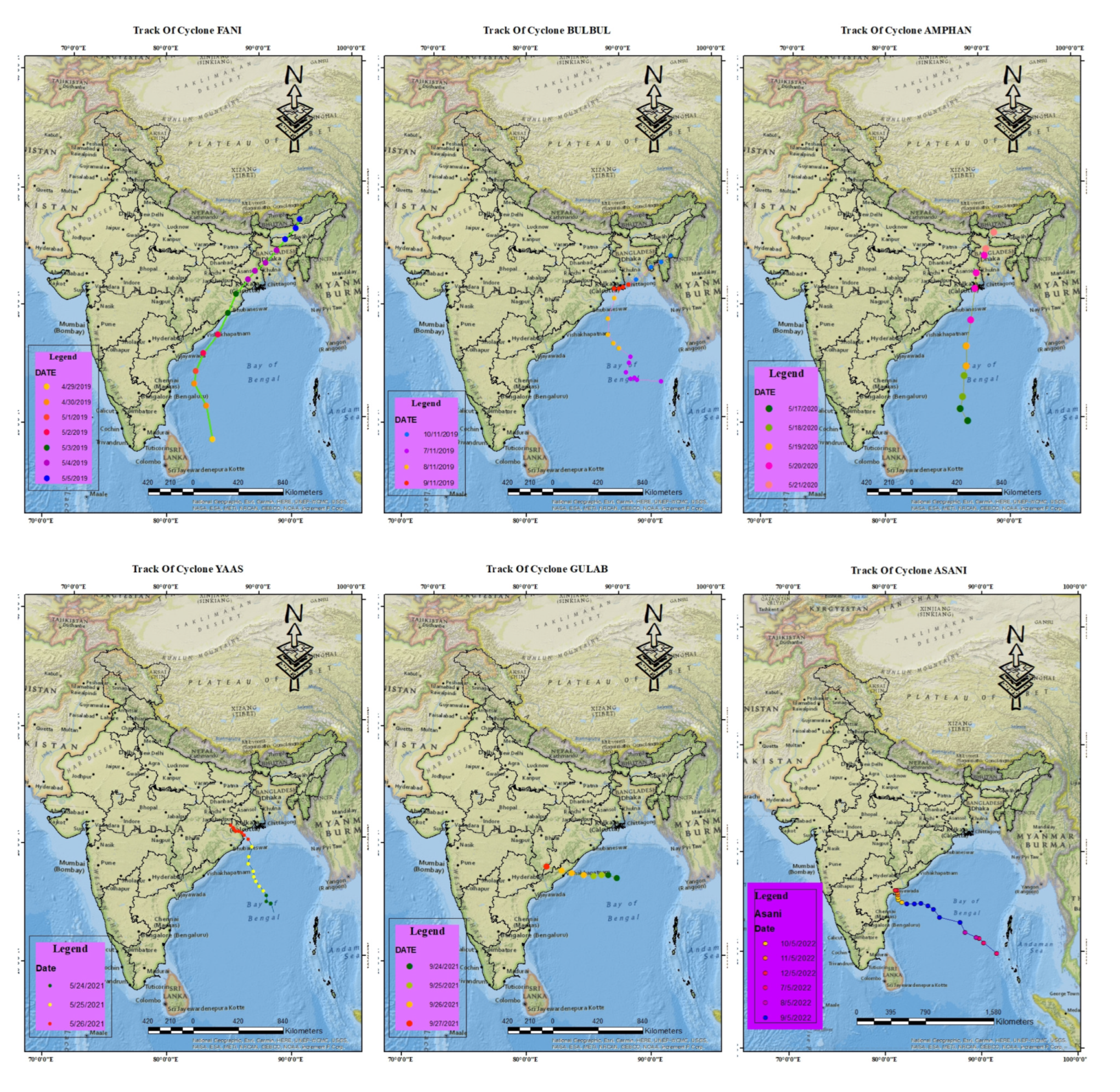
Figure 2.
Spatio-temporal temperature profiles for Cyclone Amphan at a height of 1.95 km during its progression. Panels (a), (b), (c), and (d) represent temperature distributions at 12:00 UTC on 19 May 2020, 00:00 UTC on 20 May 2020, 12:00 UTC on 20 May 2020, and 18:00 UTC on 20 May 2020, respectively. The temperature values (Kelvin) highlight the spatial variation and intensity of temperature anomalies associated with the cyclone over the Bay of Bengal and adjoining regions.
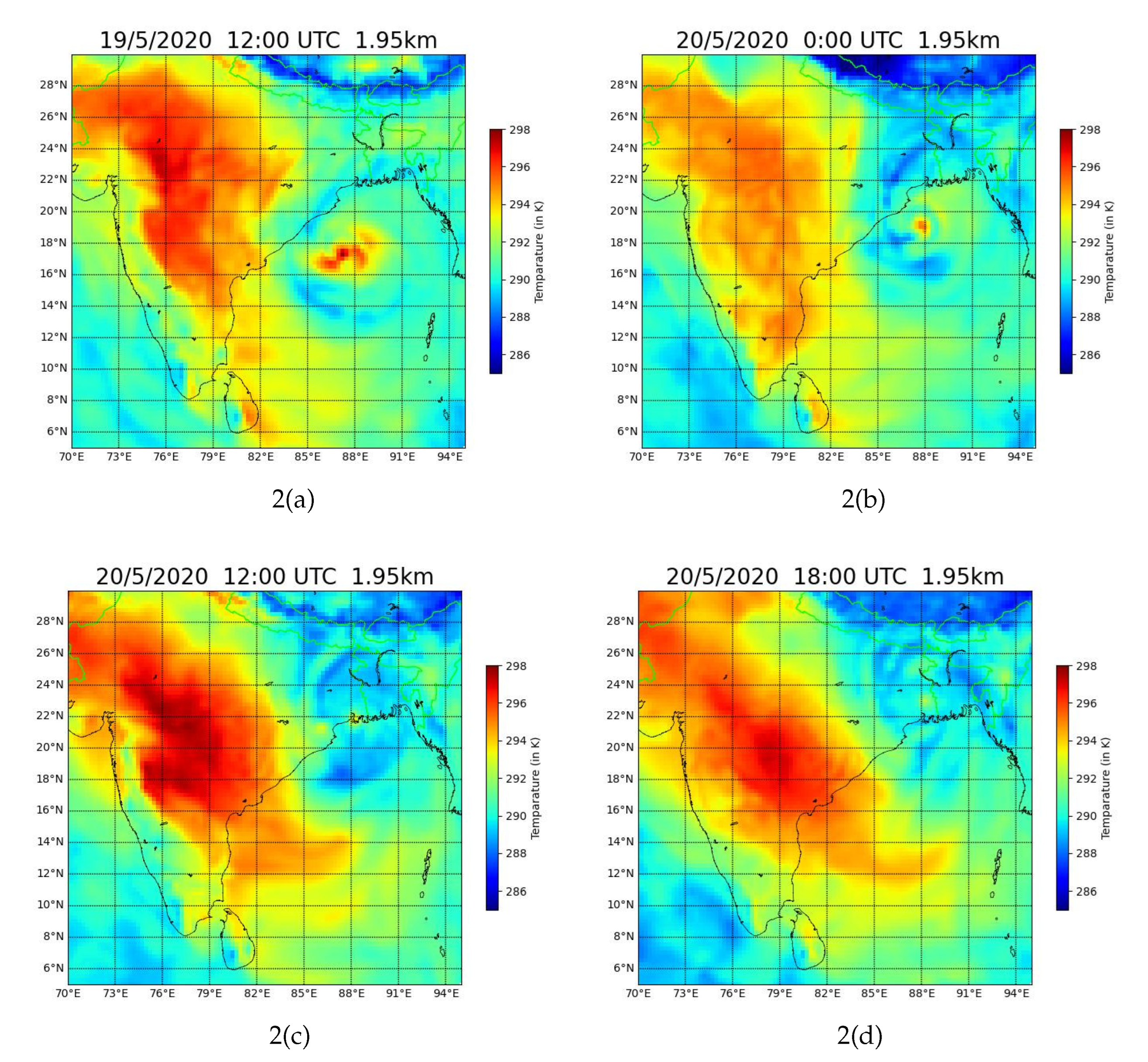
Figure 3.
Spatio-temporal variation of AGW potential energy for Cyclone Amphan at four different altitudes: (a–d) 19.31 km, (e–h) 17.66 km, (i–l) 15.79 km, and (m–p) 14.55 km. Each row represents the evolution of over time at the respective altitude, with panels showing snapshots at 12:00 UTC on 19 May 2020, 00:00 UTC on 20 May 2020, 12:00 UTC on 20 May 2020, and 18:00 UTC on 20 May 2020. The color scale, in J/kg, highlights the intensity and spatial distribution of , emphasizing the dynamics of atmospheric gravity wave activity during the cyclone’s progression.
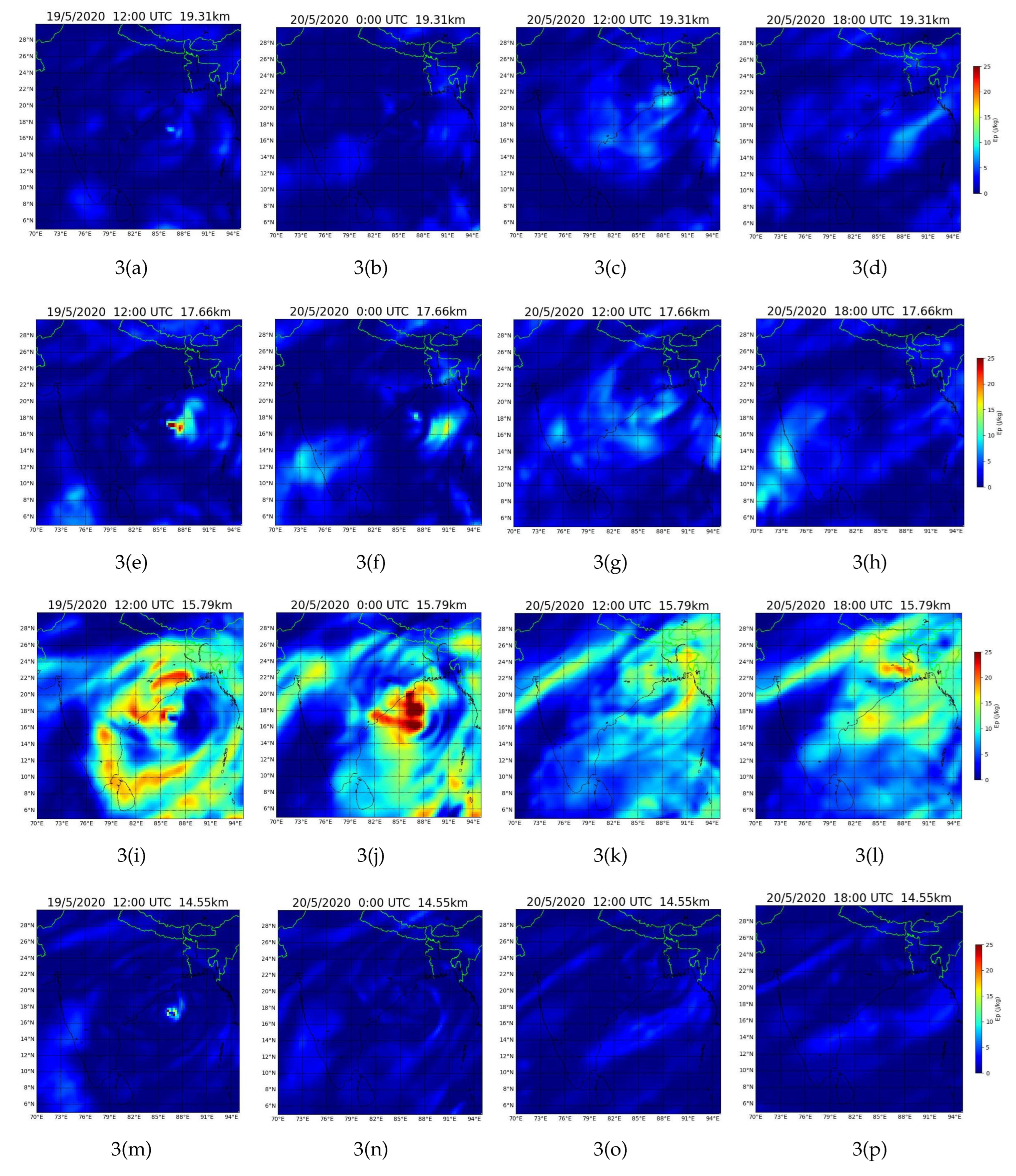
Figure 4.
spatio-tenporal profile of for cyclones Fani, Bulbul, Yaas, Gulab, and Asani) at different stages of their lifecycle. Panels (a)–(j) represent the variations across the spatial domain, showing variations in the core and surrounding areas of the cyclones at specified times and heights (denoted in km).
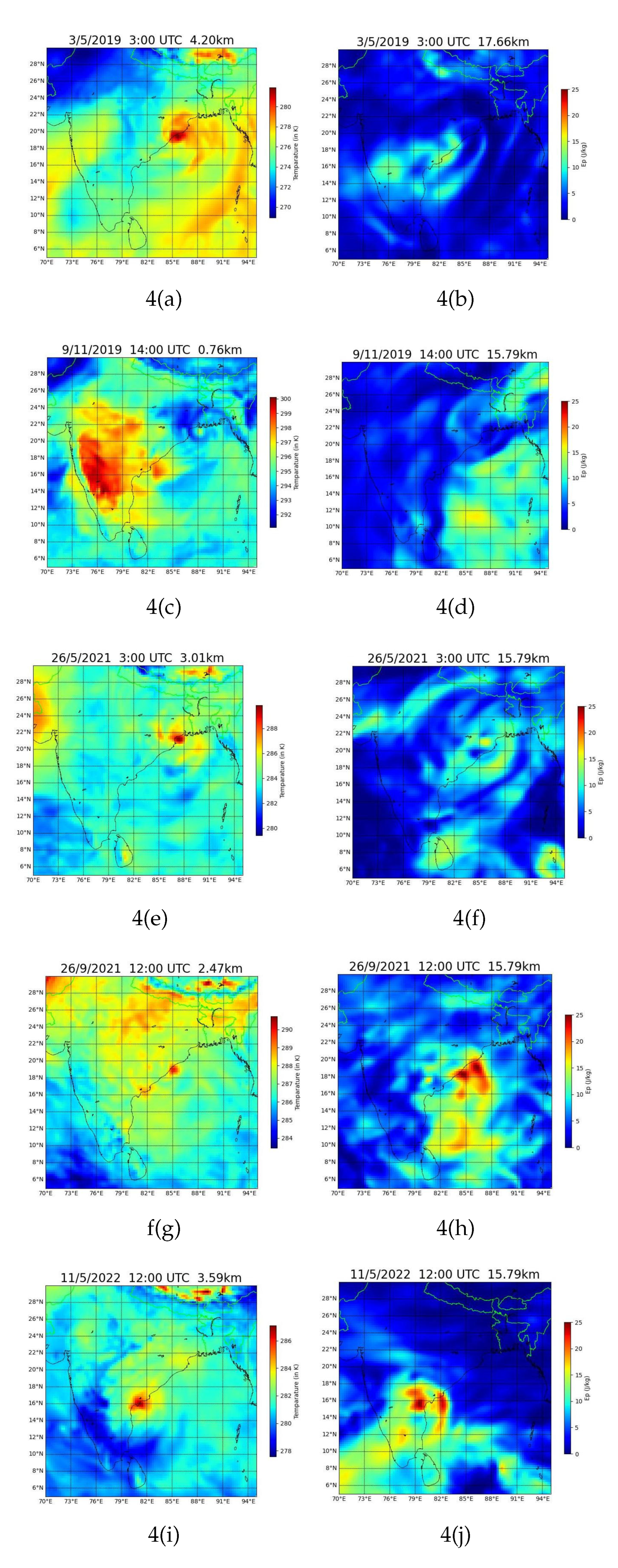
Figure 5.
Spatio-temporal variation of AGW potential energy during Cyclone Fani. Panels (a–d) represent latitudinal cross-sections of at specific times: 03:00 UTC on 2 May 2019, 15:00 UTC on 2 May 2019, 03:00 UTC on 3 May 2019, and 09:00 UTC on 3 May 2019. Panels (e–h) depict the corresponding longitudinal cross-sections for the same timestamps. The color scale indicates values in J/kg, with higher values (red and yellow regions) reflecting enhanced gravity wave activity. Significant intensification is observed around 15:00 UTC on 2 May and 09:00 UTC on 3 May, highlighting robust wave generation.
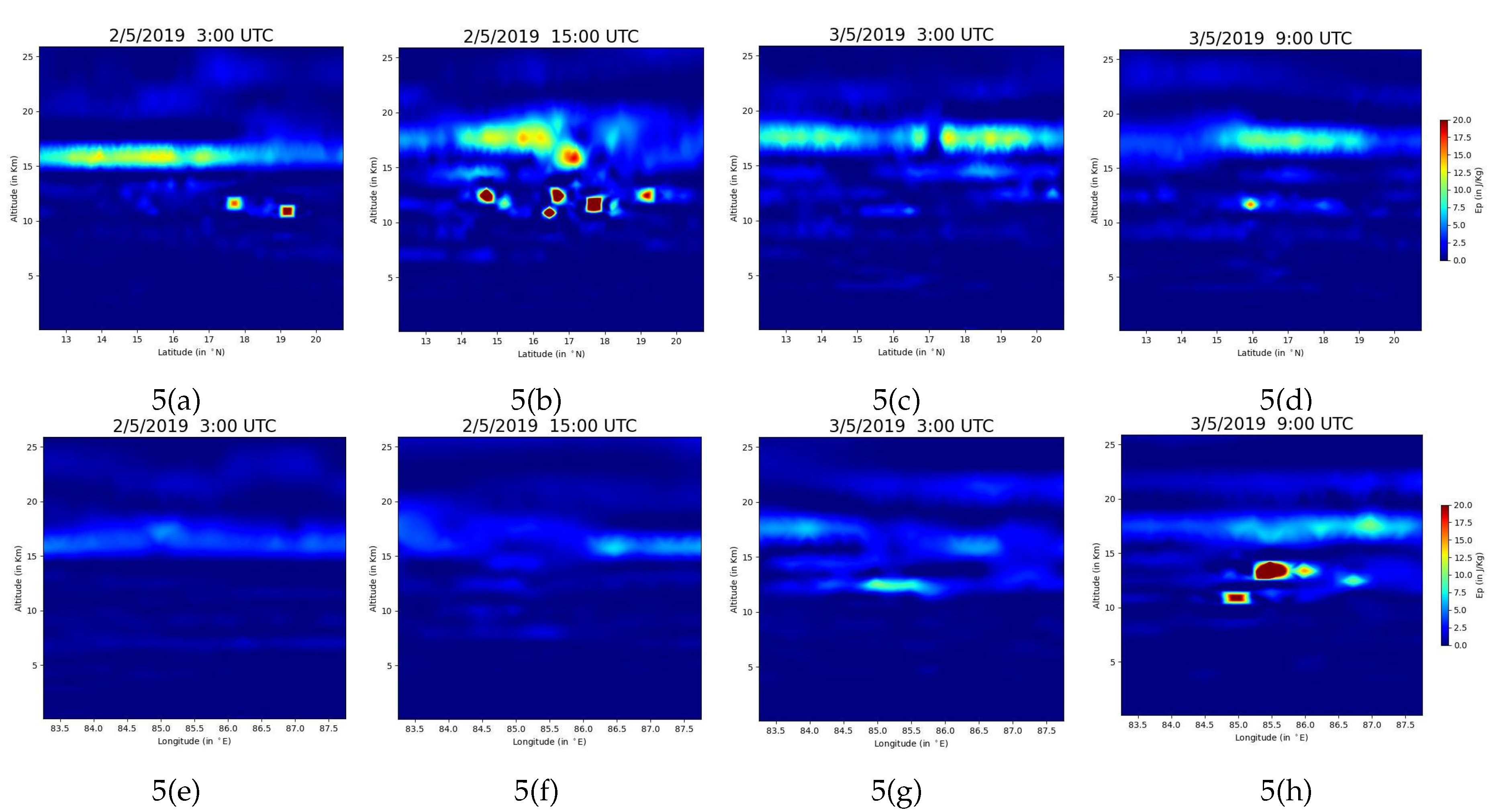
Figure 6.
Same as Figure 5 for cyclone Bulbul.
Figure 6.
Same as Figure 5 for cyclone Bulbul.
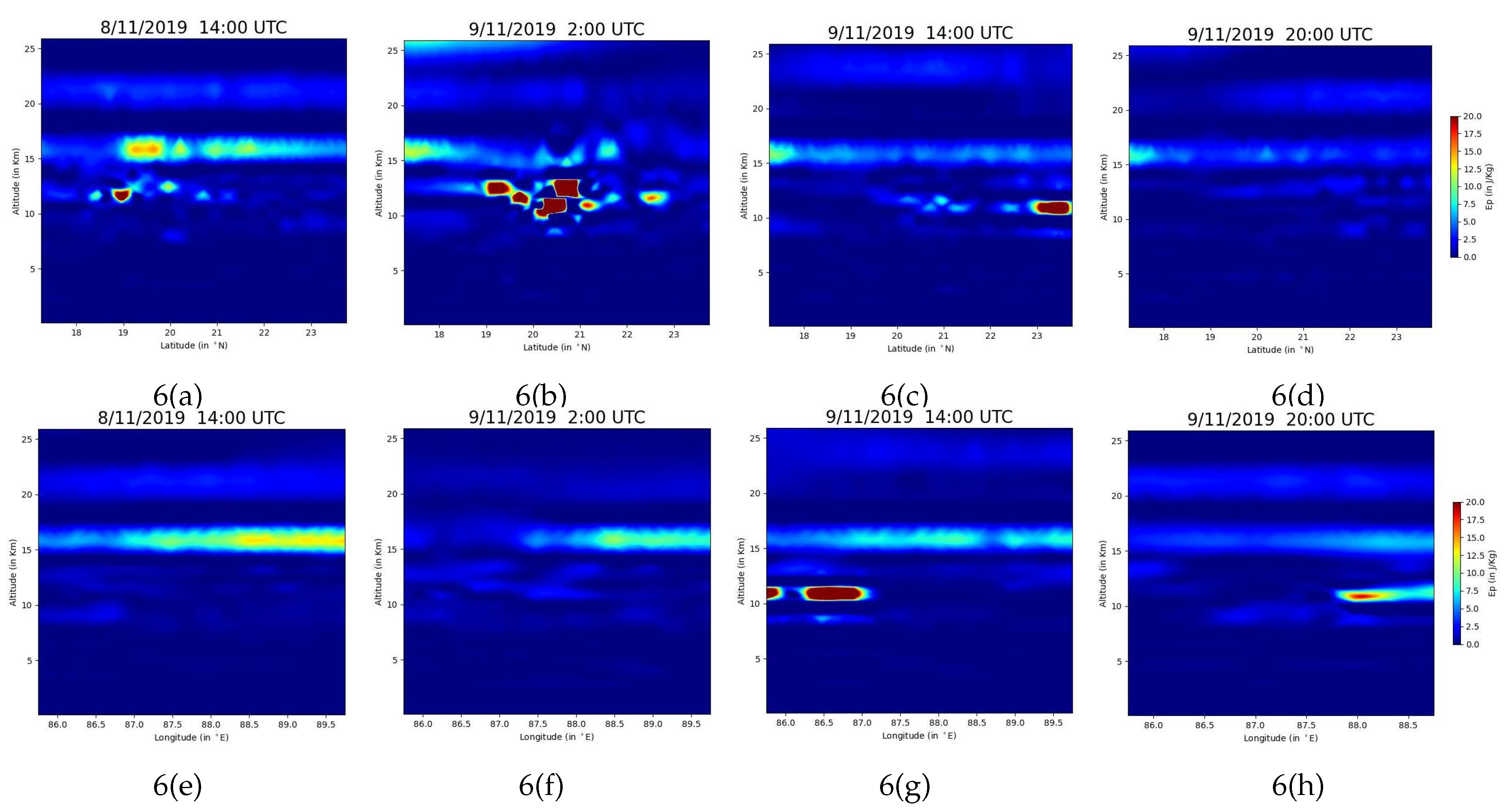
Figure 7.
Same as Figure 5 for cyclone Amphan
Figure 7.
Same as Figure 5 for cyclone Amphan
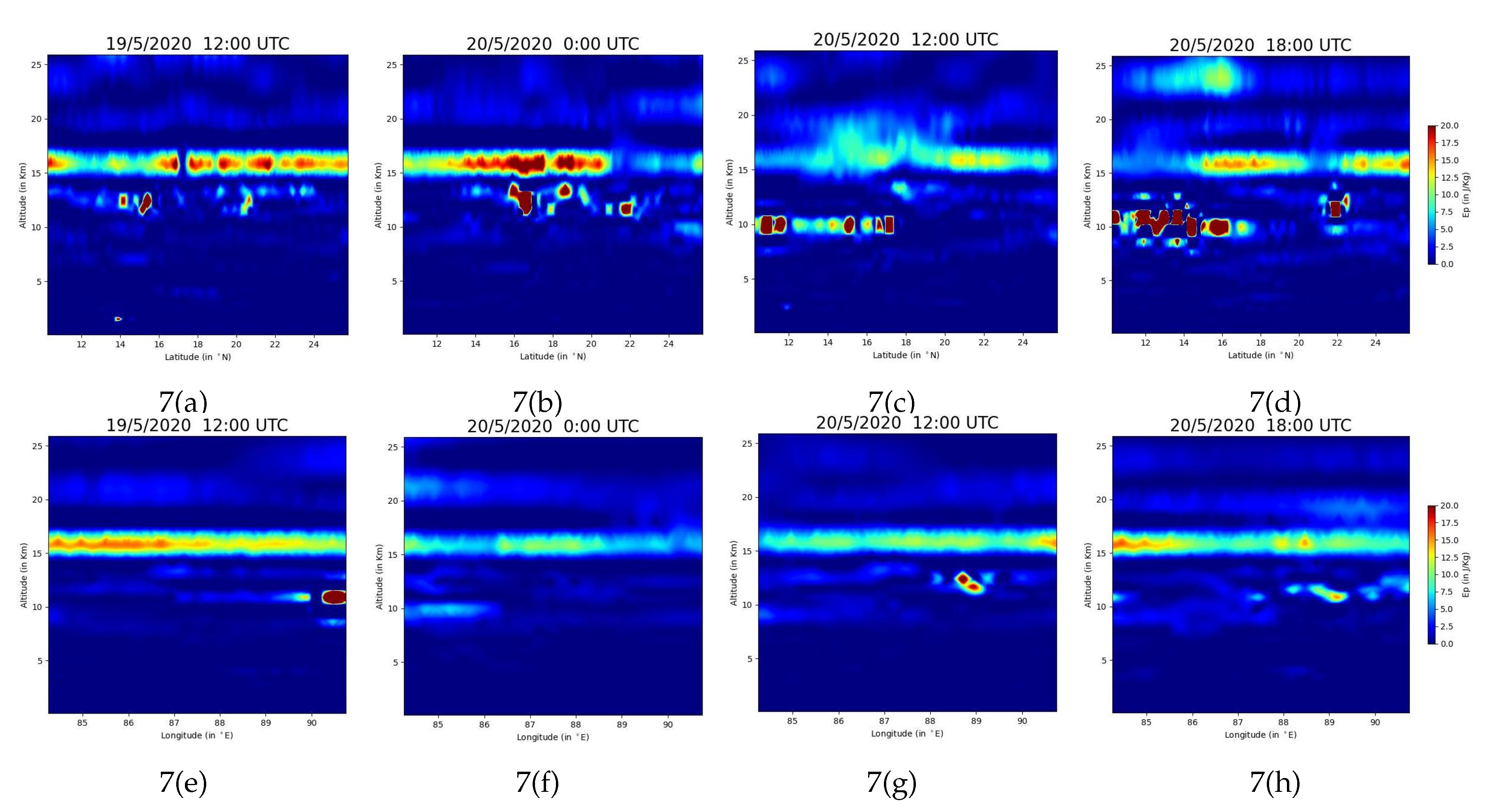
Figure 8.
Same as Figure 5 for cyclone Yass
Figure 8.
Same as Figure 5 for cyclone Yass
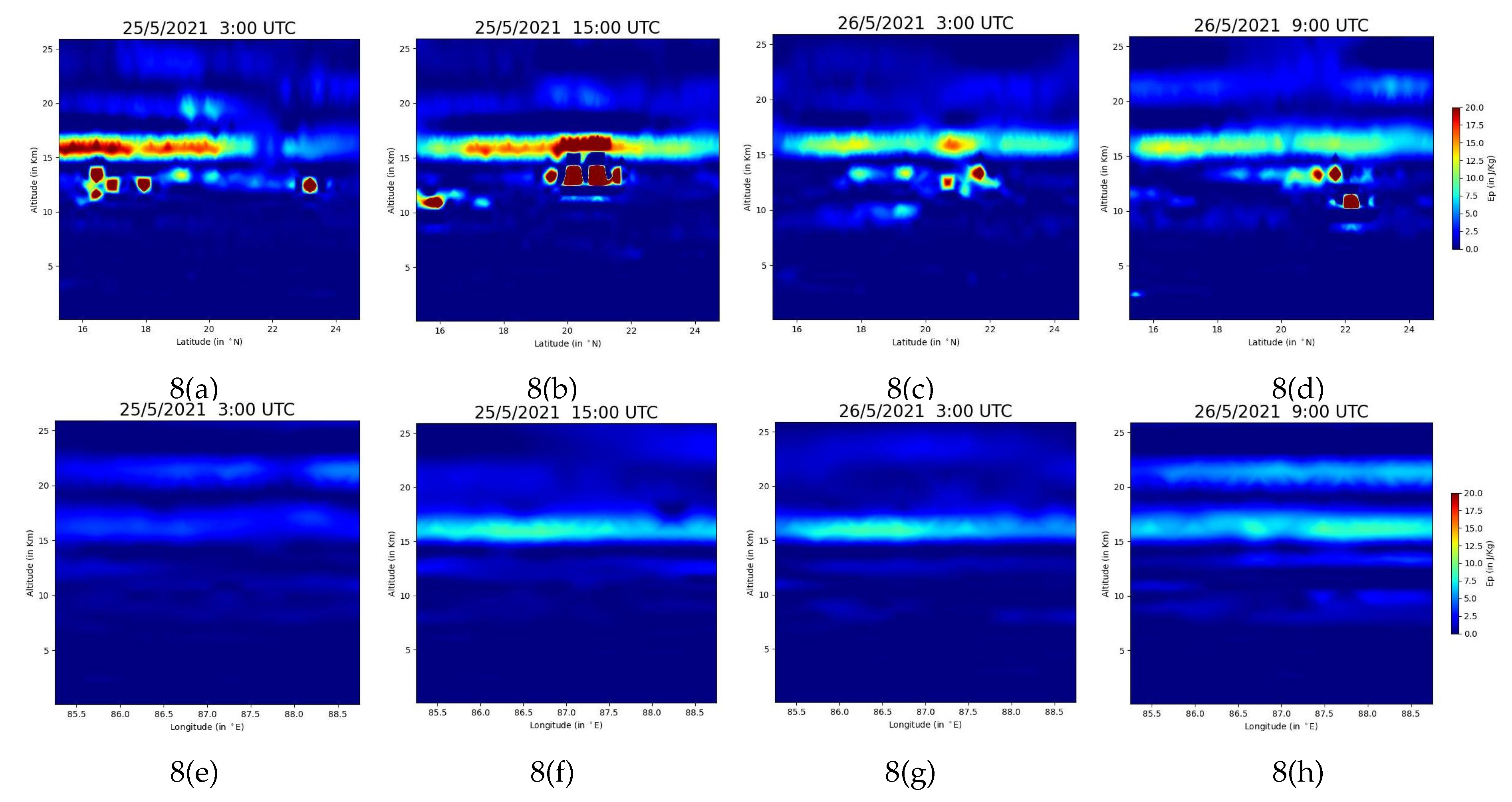
Figure 9.
Same as Figure 5 for cyclone Gulab
Figure 9.
Same as Figure 5 for cyclone Gulab
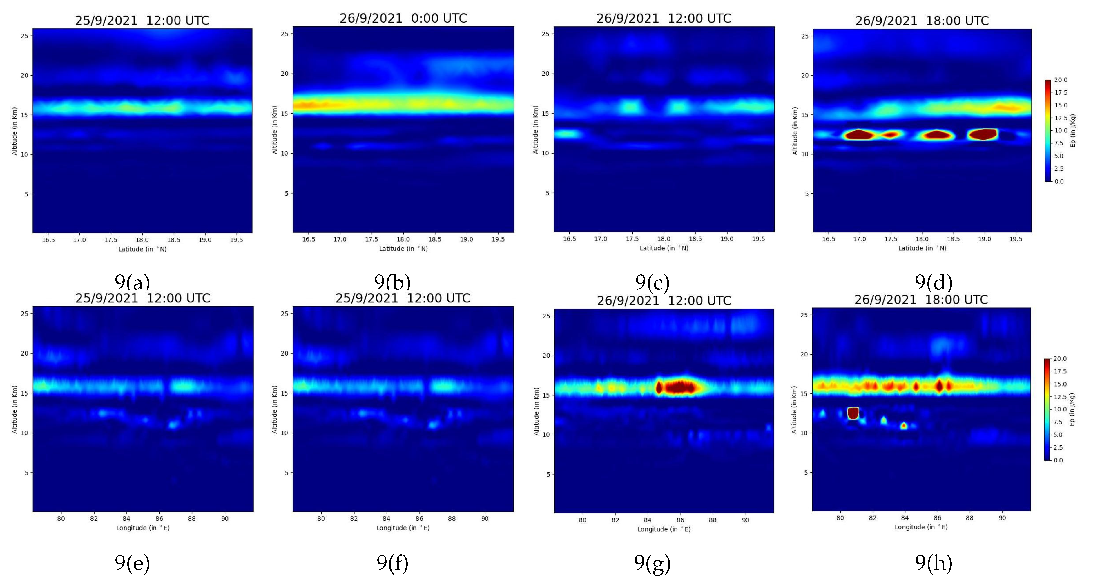
Figure 10.
Same as Figure 5 for cyclone Asani
Figure 10.
Same as Figure 5 for cyclone Asani
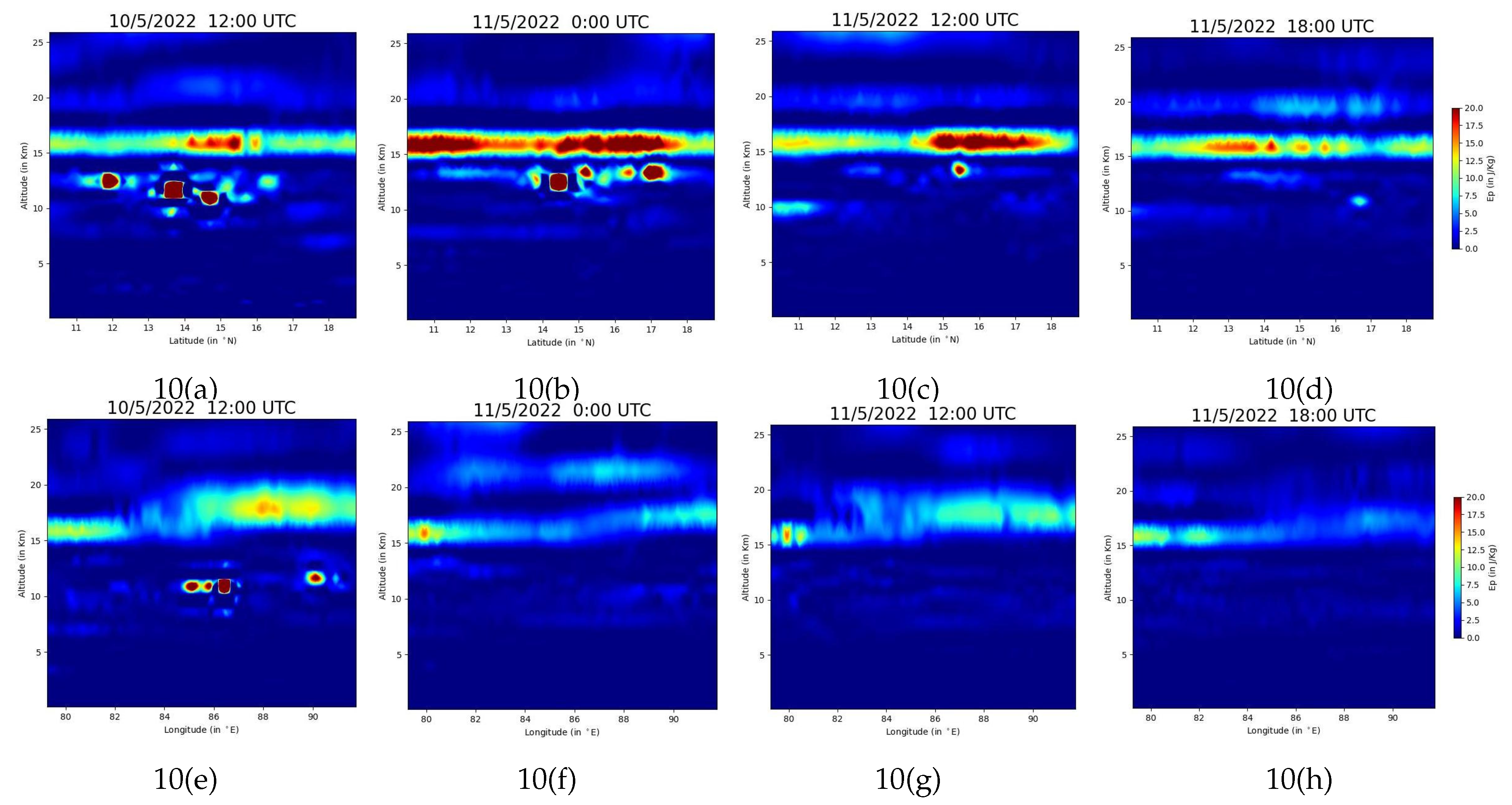
Figure 11.
Temporal variations of for cyclones Fani, Bulbul, Amphan, Yaas, Gulab, and Asani at the landfall position. The red dashed line marks the time of landfall. The plots illustrate the changes in before, during, and after landfall, highlighting the depletion near the landfall location.
Figure 11.
Temporal variations of for cyclones Fani, Bulbul, Amphan, Yaas, Gulab, and Asani at the landfall position. The red dashed line marks the time of landfall. The plots illustrate the changes in before, during, and after landfall, highlighting the depletion near the landfall location.
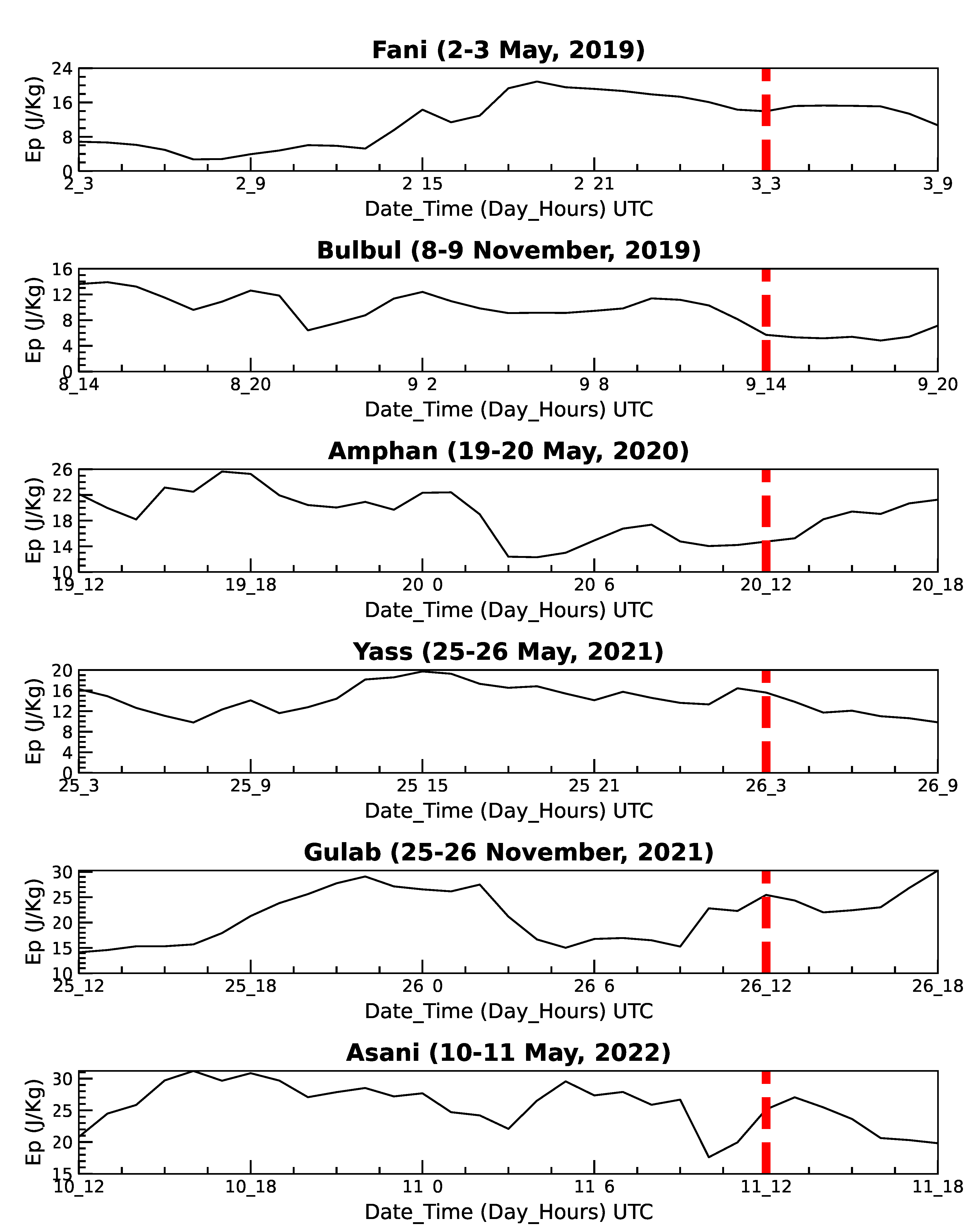

Table 1.
Summary of tropical cyclones analyzed in the study.
| Sl. No. | Date | Name of Cyclone | Landfall Position | Landfall Date | Type (IMD) |
|---|---|---|---|---|---|
| (Formed-Dissipated) | |||||
| 1 | 26/04/2019 – 05/05/2019 | Fani | Puri, Odisha | 03/05/2019 | Extremely |
| (19.8135° N, 85.8312° E) | Severe | ||||
| 2 | 05/11/2019 – 11/11/2019 | Bulbul | Sagar Island, West Bengal | 09/11/2019 | Very |
| (21.7269° N, 88.1096° E) | Severe | ||||
| 3 | 16/05/2020 – 21/05/2020 | Amphan | Bakkhali, West Bengal | 20/05/2020 | Super |
| (21.5631° N, 88.2595° E) | |||||
| 4 | 23/05/2021 – 28/05/2021 | Yaas | Bahanaga, Odisha | 26/05/2021 | Very |
| (21.3512° N, 86.7674° E) | Severe | ||||
| 5 | 24/09/2021 – 28/09/2021 | Gulab | Kalingapatnam, Andhra Pradesh | 26/09/2021 | Severe |
| (18.3387° N, 84.1211° E) | |||||
| 6 | 07/05/2022 – 12/05/2022 | Asani | Narsapuram, Andhra Pradesh | 11/05/2022 | Severe |
| (16.4330° N, 81.6966° E) |
Table 2.
Summary of the variations of each cyclones.
| Sl. No. | Name of Cyclone | Region of Maximum | Maximum | Direction of |
|---|---|---|---|---|
| intensification | Value (J/Kg) | Intensification | ||
| 1 | Fani | 16° N to 21° N, 80° E to 85° E | 13.96 | North-East |
| 2 | Bulbul | 21° N to 23° N, 88° E to 90° E | 18.21 | North-East |
| 3 | Amphan | 20° N to 24° N, 83.5° E to 88° E | 14.37 | North-East |
| 4 | Yass | 20° N to 22° N, 85° E to 87° E | 15.61 | North-East |
| 5 | Gulab | 15° N to 20° N, 83° E to 88° E | 25.45 | North-West |
| 6 | Asani | 14.5° N to 18° N, 77° E to 83° E | 25.15 | North-West |
Disclaimer/Publisher’s Note: The statements, opinions and data contained in all publications are solely those of the individual author(s) and contributor(s) and not of MDPI and/or the editor(s). MDPI and/or the editor(s) disclaim responsibility for any injury to people or property resulting from any ideas, methods, instructions or products referred to in the content. |
© 2025 by the authors. Licensee MDPI, Basel, Switzerland. This article is an open access article distributed under the terms and conditions of the Creative Commons Attribution (CC BY) license (http://creativecommons.org/licenses/by/4.0/).
Copyright: This open access article is published under a Creative Commons CC BY 4.0 license, which permit the free download, distribution, and reuse, provided that the author and preprint are cited in any reuse.


