Submitted:
31 December 2024
Posted:
03 January 2025
You are already at the latest version
Abstract
Aiming to address the vulnerability of non-stealth aircraft to radar detection due to inherent design limitations, this paper proposes a method to generate maneuvers that reduce an aircraft’s radar cross-section (RCS) value below a specified threshold. The proposed method employs control barrier functions and leverages the relationship between control inputs and the RCS. Due to confidentiality concerns, the required RCS database for the F-16 aircraft was generated through analyses performed using the created geometry. The results are compared with a virtual path that excludes RCS constraints and does not alter the aircraft’s attitude. Simulations reveal that 89.6% of the cases using the proposed method achieve a mean RCS value below the threshold, compared to only 1.26% for the virtual path. Moreover, the ratio of the time during which the RCS constraint is successfully met to the total simulation time averages over 78% across all simulations, demonstrating the method’s effectiveness in reducing the RCS value below the specified threshold.
Keywords:
low-observability
; radar cross-section
; survivability
; maneuver generation
; control barrier functions
1. Introduction
In modern aerial warfare, stealth technology has become essential for maintaining a tactical edge by allowing aircraft to evade sophisticated radar systems and operate effectively in heavily defended airspace [1]. At the core of stealth capabilities lies the reduction of radar cross-section (RCS), a critical factor determining radar detectability. By minimizing RCS, stealth technology addresses the growing challenge of radar detection, as evidenced by platforms like the F-117 and B-2. These aircraft show the substantial advantages of inherent stealth features, particularly in reducing the effectiveness of integrated air defense systems (IADS) [1,2]. However, achieving stealth is not solely reliant on structural or material technologies. Dynamic trajectory planning that minimizes RCS in real time also offers a viable approach to achieving stealth capabilities, especially for non-stealth platforms operating in contested environments.
1.1. Related Works
Historically, stealth capabilities have been achieved through aero-structural design, material technologies, and signature management tactics [3]. For example, radar absorbent materials (RAM) and shaping techniques reduce the reflected radar energy [1]. While highly effective for purpose-built stealth platforms, these methods are not applicable to legacy or non-stealth aircraft. Additionally, such structural approaches cannot adapt to changing operational scenarios or threat dynamics. Another approach involves low-altitude flight to exploit terrain masking, effectively leveraging the Earth’s curvature and natural obstructions to avoid radar detection [2,4]. However, low-altitude flight carries its own risks, including increased vulnerability to ground-based threats and terrain collision hazards. Moreover, this tactic is not always feasible in highly urbanized or geographically complex theaters of operation. Besides, many aircraft in active service, including fighter jets and transport aircraft, lack these inherent capabilities. For these platforms, operational survivability hinges on the development of innovative techniques to dynamically adapt their trajectories and reduce their radar visibility. Furthermore, the growing sophistication of radar systems has further intensified the need for advanced countermeasures. Modern radar systems employ multi-band detection, adaptive tracking algorithms, and data fusion across sensor networks to overcome traditional stealth methods [2,5]. This evolution presents a formidable challenge: how can non-stealth aircraft effectively mitigate their radar signature while maintaining mission effectiveness and flight safety? These limitations highlight the need for dynamic and adaptive stealth methodologies that can be deployed on existing non-stealth platforms. The emergence of computationally driven solutions, particularly in trajectory optimization and control systems, has paved the way for innovative stealth strategies.
In the existing literature, the dynamic trajectory optimization has emerged as a powerful tool in minimizing radar exposure by exploiting the variability in radar detection parameters. These strategies combine intelligent control and optimized route planning, enabling aircraft to adapt in real-time to radar threats [2]. Techniques like modified A-Star and sparse A-Star algorithms minimize radar exposure by implementing bidirectional sector expansions and variable step sizes, respectively, which allow unmanned aerial vehicles (UAVs) and stealth aircraft to navigate complex radar fields while maintaining stability. These methods improve survivability by dynamically adjusting the aircraft’s orientation to exploit low-detectability angles and optimize its distance from threat radars, a critical approach for high-threat environments [6,7]. Multi-phase control models are central to trajectory optimization in stealth aircraft, aiming to balance competing objectives such as minimizing radar detection, fuel efficiency, and flight time. Hybrid heuristic and adaptive pseudo-spectral methods have been developed to model radar signal characteristics alongside flight dynamics, optimizing the entire trajectory in phases. These methods effectively minimize continuous radar tracking, which is particularly valuable in regions where brief exposure intervals can make a difference in mission success.
By integrating RCS dynamics with trajectory planning, multi-phase control provides an effective way to evade radar detection without compromising on other mission-critical requirements [8,9]. Radar detection depends not only on distance but also on the relative orientation, elevation, and RCS profile of the target [5,8]. For instance, a target’s aspect angle can significantly influence its detectability, with certain orientations producing much lower RCS values than others [10,11]. By dynamically adjusting an aircraft’s trajectory to maintain low-RCS orientations relative to radar threats, it is possible to reduce detectability without the need for structural modifications. Recent advancements in radar modeling have further enhanced the potential of trajectory optimization. High-fidelity radar models now account for complex factors such as terrain masking, radar multipath effects, and environmental attenuation [4,12]. These models enable the development of more accurate and effective algorithms for stealth maneuver generation. While trajectory optimization provides a theoretical foundation, practical implementation requires real-time adaptability. In contested environments, radar threats are dynamic, with detection systems frequently shifting positions, scanning patterns, and operational modes [9,13].
Furthermore, dynamic radar environments demand adaptive path planning for sustained stealth. Adaptive algorithms incorporate factors such as radar position, angle, and power into UAV path planning to enhance survivability [9]. Additionally, machine learning methods like reinforcement learning further optimize real-time trajectory adjustments, allowing UAVs to adapt flight paths effectively in response to radar threats [13]. These algorithms provide a significant advantage in hostile environments where radar detection variables constantly shift. Accurate RCS modeling is fundamental for stealth planning, allowing for more precise avoidance of radar detection. Machine learning techniques offer robust predictions by factoring in radar wave properties and incident angles, reducing uncertainties in RCS values and improving flight path reliability [10]. These predictive models enable aircraft to navigate radar fields with greater confidence, optimizing path planning and evasion strategies.
Practical motion planning methods for stealth aircraft include strategies that minimize radar exposure during high-risk maneuvers, such as precise turning and altitude adjustments [13]. Machine learning models optimize these maneuvers to balance flight control with stealth, allowing aircraft to remain agile and maintain low-observability (LO). Techniques like multi-phase optimal control further enhance stealth by continuously adjusting flight parameters in response to real-time radar threats [12]. An integrated approach to RCS reduction combines LO technologies with adaptive motion planning techniques. In addition to static stealth designs, adaptive planning enables dynamic response to radar data in real time, enhancing the aircraft’s ability to evade radar detection throughout a mission [1,14]. By combining LO features with advanced motion planning, aircraft can maintain minimal detectability while navigating complex and evolving threat landscapes [2,11]. Advanced algorithms for real-time motion planning optimize stealth capabilities by continuously adapting flight paths in response to radar detection. Techniques derived from robotic motion planning, such as potential field methods, coordinate vehicle orientation and trajectory to avoid radar tracking, effectively managing observability [11,15,16]. These approaches integrate guidance and control systems to dynamically reduce RCS while the aircraft navigates radar-threatened environments, supporting mission success under shifting threat conditions.
The reviewed literature underscores the complexity and necessity of integrating multiple technologies and methodologies to achieve effective RCS reduction for stealth aircraft. While LO technologies such as RAM and aircraft shaping play foundational roles in reducing radar signatures, modern stealth requirements demand adaptive control and real-time path adjustments. By combining machine learning, multi-phase trajectory planning, and intelligent control algorithms, current research provides a comprehensive framework for minimizing radar observability. This multi-dimensional approach enables stealth aircraft to achieve higher survivability in hostile environments, adapting in real-time to radar detection threats and optimizing flight paths for minimal RCS.
The existing literature on stealth trajectory or maneuver optimization often employs simplified or reduced-order models that fail to capture the intricate dynamics necessary for precise trajectory or maneuver generation. Many studies rely on basic kinematic models that do not account for detailed aerodynamic effects, thus limiting their applicability to real-world scenarios [4,6,7,9,11]. By focusing solely on trajectory geometry, these approaches fall short of addressing the critical need for maneuver adaptability in highly dynamic and operationally complex airspace [5,15]. A significant limitation of many studies is their reliance on 2D or pseudo-3D trajectory models, which fail to exploit the full spatial dimensions required for effective stealth maneuvers [1,8,12]. Moreover, the fidelity of RCS database in the studies often falls short of the requirements for accurate stealth maneuver generation. Many works employ static or simplified RCS models, relying on approximations that fail to capture the real-time variability of RCS with respect to aircraft orientation and radar angle [6,7,9]. Although some studies incorporate relatively high-fidelity RCS database, they often do so without validating these models against experimental or high-fidelity databases [4,10] and they often limit the planning domain to fixed altitudes or simplified geometries, thereby reducing their relevance in complex operational scenarios [13]. Consequently, these studies do not provide sufficient fidelity for generating realistic penetration trajectories, particularly for non-stealth platforms operating in variable threat landscapes [2,16]. The absence of a comprehensive integration of RCS dynamics with maneuver planning further weakens the practicality of these approaches, as they cannot adapt to radar threats that depend on rapid changes in aircraft orientation [12,15]. Another point of concern, the control surface deflections, a critical factor in achieving precise stealth maneuvers, are neglected in most studies [1,8,13,16]. Without explicit consideration of control surface deflections, these methods cannot generate stealthy trajectories that are both realistic and executable under operational constraints. Finally, the previous studies predominantly focus on precomputed path planning rather than real-time maneuver generation, which is a critical limitation in dynamic radar environments. Algorithms like A-Star and sparse A-Star offer optimal solutions for static or semi-dynamic scenarios but lack the adaptability needed for continuously changing radar threats [6,7,9]. By focusing primarily on static optimization, these methods fail to address the need for continuous trajectory adjustment, a cornerstone of effective stealth operations in modern contested airspace [12,15].
1.2. Contributions & Organization
This study aims to develop a comprehensive framework that overcomes the limitations of existing stealth maneuver generation methods by employing Control Barrier Functions (CBFs) to dynamically enforce radar observability constraints. The proposed approach integrates high-fidelity aerodynamic modeling, considers the effects of control surface deflections, and incorporates real-time adaptability to enable non-stealth platforms to achieve low radar detectability. By dynamically adjusting angular rates to maintain compliance with RCS thresholds while optimizing survivability, this framework bridges the gap between theoretical advancements and practical implementation. Ultimately, this paper sets a foundation for adaptive stealth strategies that enhance the operational effectiveness of non-stealth aircraft in contested environments. The contributions of this study are itemized;
- This study introduces a CBF-pilot design to generate stealthy maneuvers based on high-fidelity flight dynamics model that captures the complex behavior of non-stealth platforms, contrary to most of the existing studies using simplified kinematic flight dynamics model. The utilization of high-fidelity flight dynamics model provides an accurate representation of flight dynamics, allowing for better assessment of radar observability under various and realistic operational conditions.
- By incorporating the effects of control surface deflections on RCS, the study ensures that these factors are properly accounted for in stealth maneuver planning. This integration enhances the realism of the model and improves the ability to generate effective stealthy maneuvers.
- The framework adapts in real time, dynamically adjusting flight maneuvers to maintain stealth characteristics. This real-time adaptability ensures that non-stealth platforms can continuously optimize their flight paths to minimize radar detectability while meeting operational constraints.
The remainder of the paper is organized as follows. First, Section 2 explains the problem then following Section 2.1 provides the necessary background for the study, including modeling of nonlinear flight dynamics, design of flight control laws. In Section 3, the radar cross-section analysis methodology is presented. Section 4 presents the design of the stealth maneuver generator using control barrier functions. In Section 5, the proposed strategy is evaluated through various scenarios and Monte Carlo simulations. Finally, the results and potential future research directions are discussed in Section 6.
2. Problem Description and Preliminaries
Radar-penetration maneuvers are critical and among the most realistic operations, typically occurring under highly challenging and intensive conditions. What makes radar-penetration maneuvers particularly realistic is the increasing sophistication of radar systems. This sophistication underscores the need for innovative approaches to enhance the ability of aircraft, especially non-stealth platforms, to evade detection during tactical maneuvers. Non-stealth aircraft, due to their inherent design limitations, are especially vulnerable to radar detection in such operations. This heightened detectability drastically reduces their survivability, as they are more likely to be targeted and neutralized. Addressing this challenge requires a deep understanding of the interaction between radar cross-section characteristics and aircraft maneuvering capabilities, which forms the foundation of this study. At this point, the research question arising from this context is: How can non-stealth aircraft execute tactical maneuvers that minimize their detectability by radar systems while simultaneously enhancing their survivability? Answering this question involves exploring methods to temporarily transform non-stealth aircraft into low-observable platforms during critical phases of a mission. Thus, the illustration in Figure 1 principally depicts the radar-penetration maneuver scenario as the foundation of the proposed method.
The scenario illustration demonstrates that the aircraft must pass through the radar coverage zone. In the absence of radar, the aircraft would have followed a straight flight path to pass over the zone. Consequently, this straight flight trajectory is considered the virtual (or ideal) path, meaning that the angular rates remain zero throughout the path, i.e., . However, the presence of radar necessitates reshaping the virtual path to account for the aircraft’s radar cross-section. The problem can thus be formulated as an optimization problem for motion planning, aiming to adhere to radar cross-section constraints while staying as close as possible to the virtual path.
The methodology underlying this approach is grounded in the use of an RCS database, belonging to a non-stealth aircraft. Building upon this foundation, the study leverages control barrier functions to enforce constraints on RCS values during maneuver execution by commanding angular rates, : p, q and r. By ensuring that the aircraft’s RCS does not exceed predetermined thresholds, the proposed method enables the generation of stealthy maneuvers that enhance survivability. In summary, this study addresses a pressing challenge in modern aerial operations by developing a methodology to reduce the detectability of non-stealth aircraft during radar-penetration maneuvers.
2.1. Preliminaries
The necessary background for the subsequent sections is established in this section, including high-fidelity flight dynamics modeling, control augmentation system design using incremental nonlinear dynamic inversion, and the fundamentals of the control barrier functions.
2.1.1. Flight Dynamics Model
The baseline aircraft is an F-16, whose nonlinear flight dynamics model is adopted from [17]. The major components of the flight dynamics model are detailed in the subsequent sections.
Equations of motion
The axes frame of the baseline aircraft is depicted in Figure 2.
The set of nonlinear flight dynamics equations is presented in Equation (1), including translational and rotational dynamics, and translational and rotational kinematics, respectively.
where u, v, and w denote the components of the body velocity, while p, q, and r represent the angular rate components in the body frame. The navigational position is specified by , , and , and the orientation is described by the Euler angles , , and . The force components acting on the body frame are given as , , and , with L, M, and N representing the roll, pitch, and yaw moments, respectively. Additionally, m signifies the mass of the aircraft, while , , , and define the aircraft’s moments of inertia.
Aerodynamics & Actuators
The aerodynamic database and the corresponding formulations are directly adopted from [17]. There are three body force coefficients, i.e., , , and , and three moment coefficients, i.e., , , and . The aerodynamic coefficients depend on relevant flight states, such as the angle of attack (), sideslip angle (), and control surface deflections, including horizontal tail deflection (), aileron deflection (), and rudder deflection ().
Additionally, the actuator dynamics are modeled as a first-order system that accounts for time constants, rate limitations, and position saturation constraints, as outlined in [17]. Specifically, the time constant for each control surface is set to . The rate saturation limits are for the horizontal tails, for the ailerons, and for the rudder. Likewise, the position saturation limits are for the horizontal tails, for the ailerons, and for the rudder.
2.1.2. Flight Control Law Design
The control augmentation system employs a single-loop angular rate control law based on incremental nonlinear dynamic inversion (INDI). The derivation of this control law is simplified by the control-affine structure of Euler’s equations of motion, as expressed in a decomposed form in Equation (2).
where , S, b, and represent the dynamic pressure, wing area, wing span, and mean aerodynamic chord, respectively. Additionally, denotes the control effectivity matrix, which contains the moment coefficient derivatives with respect to the control surface deflections at the current instant, with n indicating the number of control surfaces. The INDI control law for regulating the angular rates is derived as shown in Equation (3).
where the subscript ′0′ denotes the current state and represents the virtual input to be designed. The final form of the control law is provided in Equation (4).
where denotes the control surface deflections, corresponding to the horizontal tail, aileron, and rudder, respectively. Additionally, since there are three control surfaces (), the control effectivity matrix is a square matrix, and it remains invertible unless it is rank deficient. Furthermore, the virtual input is given by Equation (5).
where , , and are the gains for the roll, pitch, and yaw channels, respectively. The provided expressions outline the necessary generation of control surface deflections in response to the pilot commands , , and .
2.1.3. Control Barrier Functions
A super-level set at level c, which maps the value of a function () over c is given in Equation (6) using the safe set definition from [18].
where is safe set, is the boundary and is the interior of the safe set. In addition, , then defines the safe region while defines unsafe region. Time derivative of is given in Equation (7) using Lie derivative notations.
Definition 1.
3. Radar Cross-Section Quantification
The radar cross section (RCS) measures a target’s ability to reflect radar signals back toward the radar receiver. RCS compares the strength of the signal reflected by a target to that of a perfectly smooth sphere with a cross-sectional area of 1 . RCS, denoted as , value of a target is defined in Equation (10).
where is the incident power density measured at the target, is the scattered power density seen at a distance r away from the target, r is the distance from target. Additionally, RCS is often expressed on a logarithmic scale for clarity and practicality, as defined in Equation (11).
where represents the RCS measured in square meters (), while dBsm provides a logarithmic representation of the RCS in decibels.
3.1. Methodology
The RCS database for a specific aircraft may not be available due to confidentiality issues. Therefore, developing an approach regarding the observability during a radar penetration maneuver primarily requires generating a sufficiently accurate representation of the RCS characteristics through detailed analyzes. The reliability of these analyzes depends on several factors, such as the accuracy of the modeled aircraft geometry, the quality of the mesh, and the solver type. It is important to note that even if the geometry, including mesh options, and analysis parameters are chosen appropriately, the generated RCS characteristics may still differ from the exact profile. This discrepancy can be attributed to factors such as incomplete knowledge of the materials used in the aircraft, surface treatments, and the effects of coatings [1,3]. Yet, in this study, the primary goal of generating the RCS database is to achieve a close approximation of the real RCS profile, enabling the demonstration of the proposed maneuver generation approach’s capabilities. For this purpose, primarily, the digital F-16 geometry with movable control surfaces was modeled in Blender®, a computer-aided design software, and then meshed using a total of 20000 elements. The digital geometry and the generated mesh are demonstrated in Figure 3.
The RCS analyzes were performed in ANSYS® using the Shooting and Bouncing Rays (SBR) method at 3 GHz [20] with the generated mesh. RCS analyzes are characterized by the azimuth and elevation angles. These angles represent the relative orientation of the aircraft with respect to the radar position, as depicted in Figure 4.
By definition, the range of the angle is [-180°, 180°], whereas the range of the angle is [0°, 180°]. Therefore, a comprehensive RCS analysis should cover all combinations within these ranges. Furthermore, however, analyzing only the possible combinations of and angles is insufficient to construct a high-fidelity RCS database, as the control surfaces are movable. Thereby, the deflection in the control surfaces changes the spatial geometry and so do the RCS characteristics. To address the concern regarding the fidelity of the constructed database, the geometry with control surface deflections must also be modeled, and the incremental addition of the control surface deflections should be included in the RCS database. Consequently, the RCS analysis points should be defined as follows: within the range , within the range , and the aileron (), horizontal tail (), and rudder deflections () within the range , with .
3.2. F-16 Radar Cross-Section Characteristics
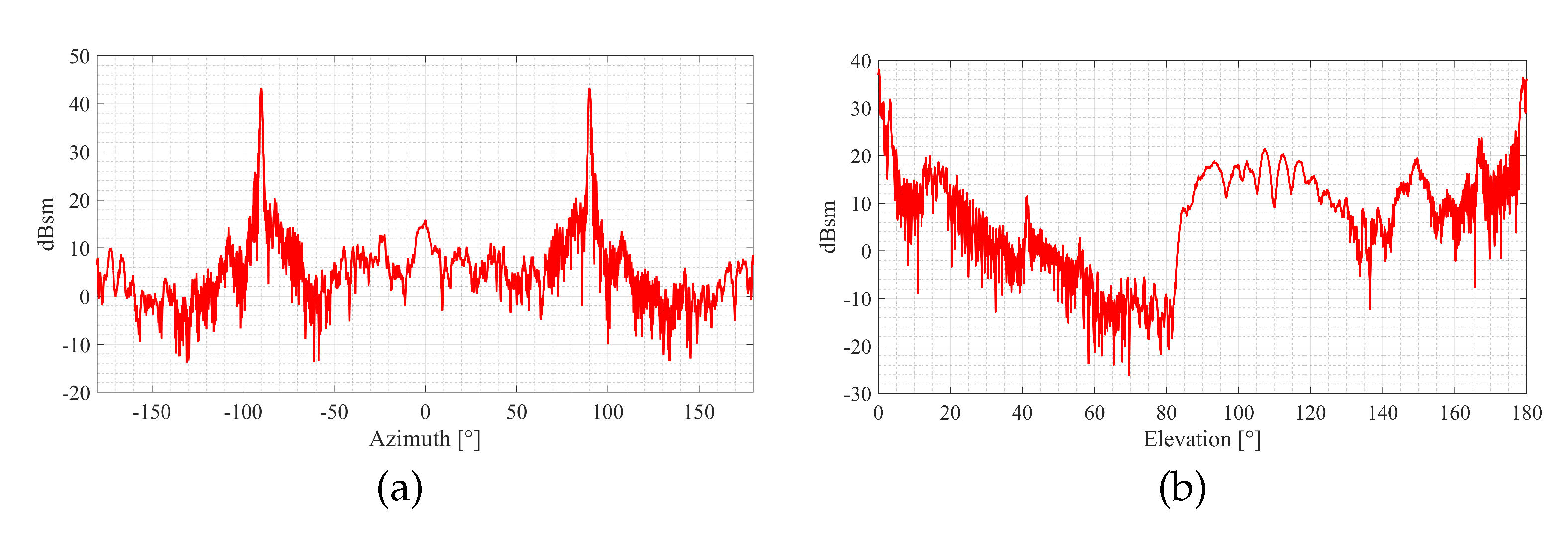
Building on the previously discussed analysis methodology, the variation in the RCS characteristics is illustrated in Figure 5 by keeping either the elevation or azimuth constant at values of and , respectively.
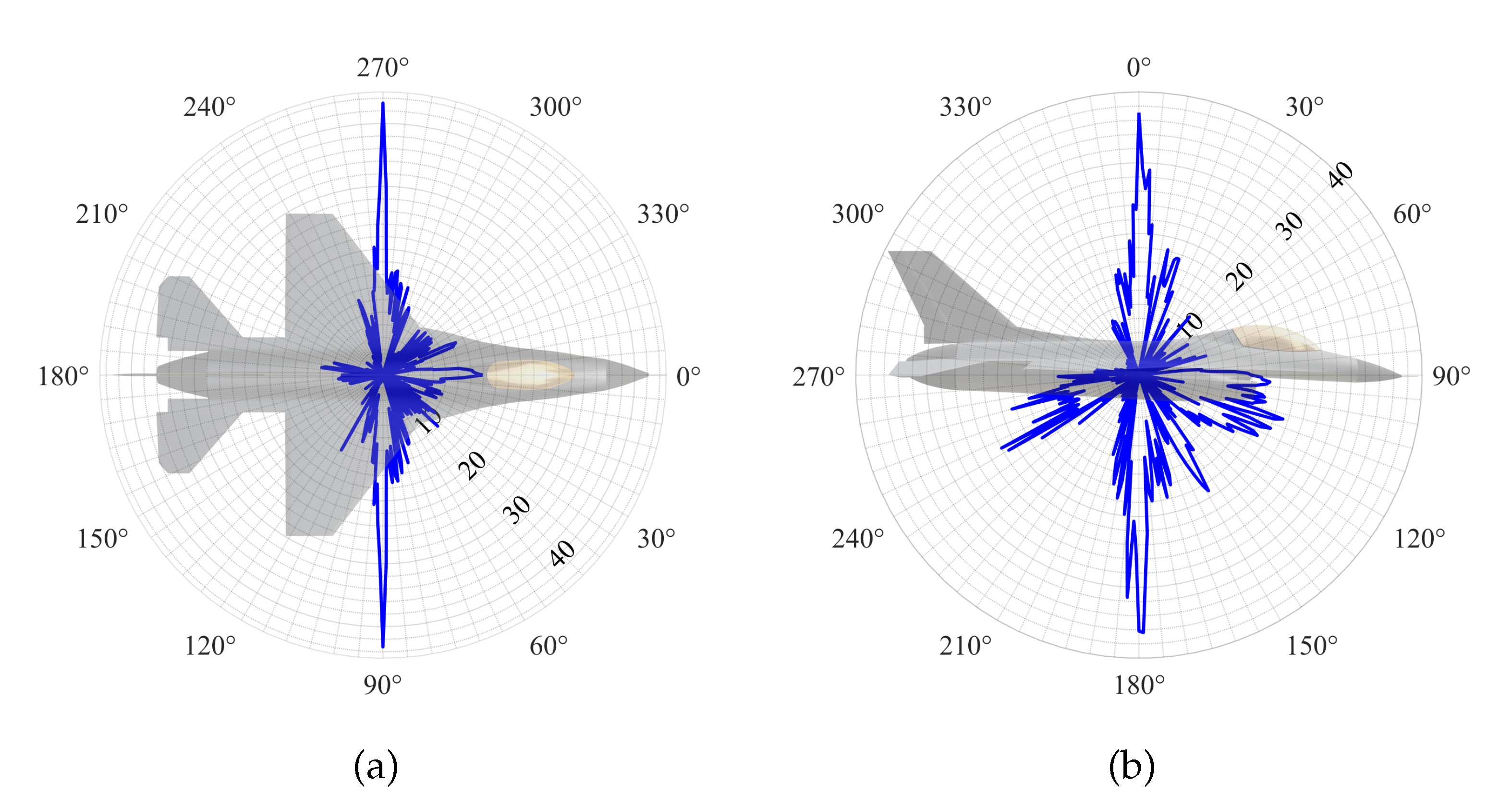
The polar representation of the corresponding RCS variation is depicted in Figure 6 for the sake of creating visual intuition.
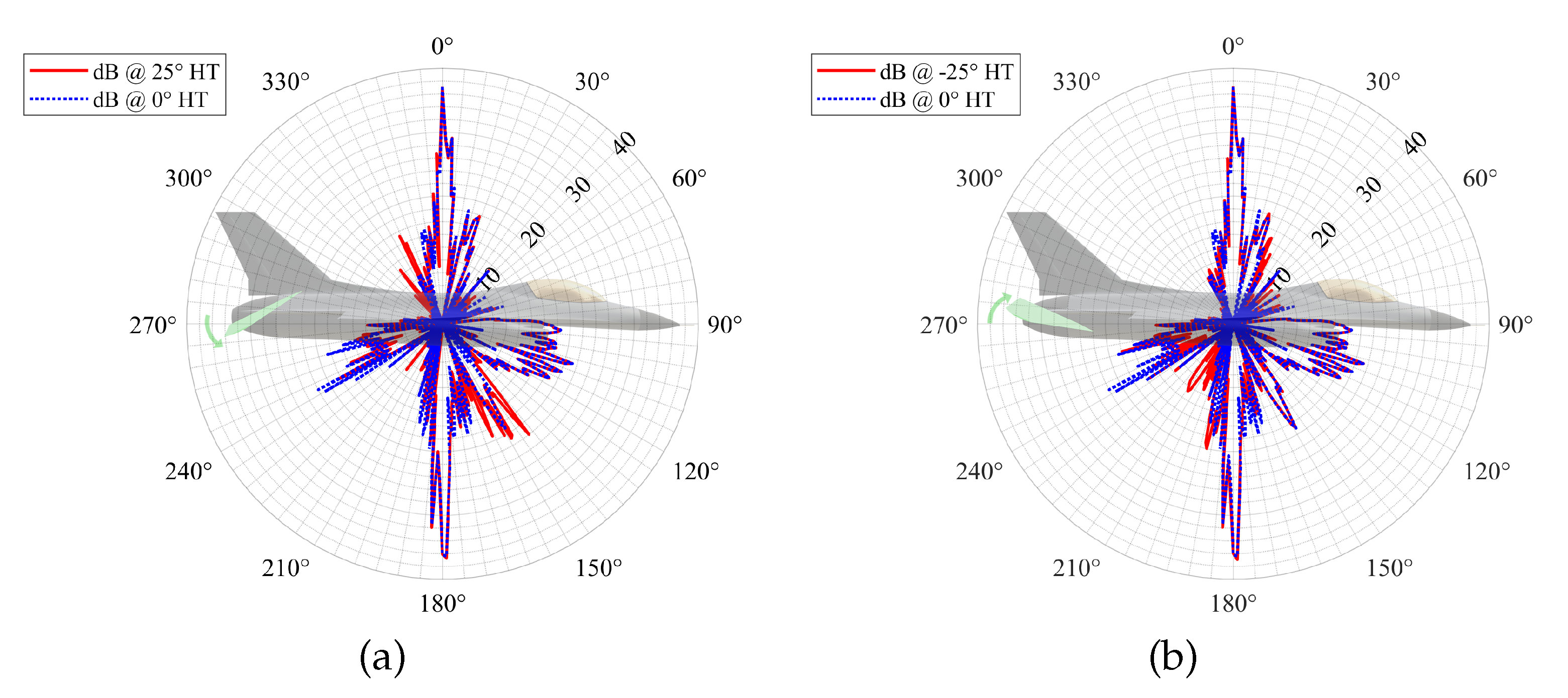
The effects of the horizontal tail deflection on the RCS characteristics are depicted in Figure 7 comparatively.
The results indicate that while there is minimal variation in RCS values when the aircraft is tracked from the frontal aspect of the radar, a noticeable increase occurs when the radar rays encounter the horizontal tail at a perpendicular angle. Specifically, for a horizontal tail angle, the RCS value increases by approximately at an elevation angle of . Similarly, for a horizontal tail angle, the RCS value rises by about at an elevation angle of . As an adjunct instance, the rudder deflection effects on the RCS characteristics are illustrated in Figure 8.
Subsequently, the generated RCS database is embedded in a 5D look-up table, where each dimension corresponds to , , , , and , with linear interpolation and a cut-off for extrapolation.
As the final step, the conversion between the aircraft orientation (, , ) and the relative orientation (, ) should be introduced since the RCS database is a function of the relative orientation. Assuming the radar is always facing the aircraft, a conversion method can be developed by using the positions of the F-16 and the radar, and the attitude angles of the F-16. First, the distances between the radar and the F-16 are calculated and converted to the body frame of the aircraft, as described in Equation (12).
where is the position of the aircraft, is the position of the radar, and represents the direction cosine matrix from the body frame of the F-16 to the inertial frame with ZYX order rotation and is formulated as presented in Equation (13)
where bank angle , pitch angle and yaw angle represents the attitude angles and c and s are the cosine and sine operators respectively. Then, the and angles are determined by converting from the cartesian to the spherical coordinate system using the Equation (14).
where and describes the components of in Equation (12).
At the end of the section, the methodology for generating the RCS database and its direct correspondence to the aircraft’s motion have been elaborated, providing a foundation for the subsequent section, which introduces the stealth-maneuver generator design.
4. Stealth-Maneuver Generator
The primary principle of stealth-maneuver generator design is to maintain the aircraft’s RCS below a predetermined maximum allowable threshold during radar-penetration. In this regard, the stealth-maneuver generator is required to generate , , and ; therefore, the RCS should be formulated and decomposed in a manner that ensures the angular rates are observable. Fortunately, the RCS is a function of aircraft attitude angles (, , and ), implying that the angular rates can be revealed provided that an appropriate barrier function is established. A barrier function is then designed, as presented in Equation (15).
where is the predetermined maximum allowable RCS value. It is obvious that , and . Thus, the time derivative of the barrier function is . At this point, an expansion of the time derivative of the barrier function should be given, as presented in Equation (16).
where , , and represent the RCS derivatives with respect to the bank angle, pitch angle, and yaw angle, respectively. Provided that the RCS database is available, these partial derivatives can be calculated using either the central difference method—preferred in this study—or formulating the RCS as a polynomial function.
Subsequently, to derive the angular rates from the RCS dynamics, the bank, pitch, and yaw dynamics should be expressed as , , and , respectively. It is quite straightforward since the attitude dynamics are represented through a transformation matrix and angular rates, i.e., . By recalling the rotational kinematics given in Equation (1), the required decomposition for the bank, pitch, and yaw dynamics can be performed as shown in Equation (17).
Attentive eyes will notice that the components of , , and are row elements of the transformation matrix . Subsequently, the RCS dynamics can be represented in the form of , as given by Equation (18).
Consequently, the CBF constraint can be described as given in Equation (19).
where is the design parameter to be chosen properly. As a consequence, the final form of the stealth-maneuver generator formulation for commanding angular rates is presented in Equation (20).
The constructed formulation enables the stealth-maneuver generator to command angular rates (, , and ) that closely follow the reference angular rates (, , and ) corresponding to the virtual path, while ensuring compliance with the radar cross-section constraint. Furthermore, the generated angular rate commands must remain within the interval , considering the admissible and allowable angular rate limits specific to the aircraft. The overall proposed architecture is depicted in Figure 9.
5. Simulations and Results
The simulation scenarios and methodologies employed to evaluate the proposed CBF-based framework for stealth-maneuver generation for non-stealth aircraft are presented. Two primary scenarios were designed: radar-penetration maneuver and radar-evasive maneuver, each developed to simulate operationally realistic and dynamically challenging conditions. High-fidelity flight dynamics model, detailed RCS analyzes, and real time control algorithm were integrated to simulate these scenarios. Additionally, Monte Carlo simulations were conducted to assess the robustness and consistency of the proposed approach across a range of initial conditions. This structured evaluation provides a comprehensive analysis of the proposed methodology.
5.1. Scenario-1: Radar-Penetration Maneuver
This scenario simulates a case where radar-penetration is unavoidable and ends when the aircraft reaches the same position with the radar on the North axis. The objective of this scenario could be to gather information around the radar base for a reconnaissance mission or to neutralize targets near the radar position. The cruising aircraft’s initial speed is 0.8 Mach, with a 0° path angle and a 30° heading, at an altitude of 2000 m. The radar position is set at [5000,0,0] with a range of 5000 m. The maximum allowable RCS value is set at 0 dBsm, and the resulting RCS history is presented in Figure 10.
The proposed methodology is compared with the virtual path, which has no RCS constraints and does not change its attitude, as shown in Figure 10. For both results, the initial RCS values exceed the threshold for a brief period; however, the proposed method successfully manages to satisfy the constraint through the generated maneuvers. Over 10 seconds, the F-16 is able to maintain its RCS value below 0 dBsm, with only minor violation observed afterward. In contrast, the virtual path consistently produces higher RCS values. For the virtual path, the F-16’s RCS value reaches nearly 25 dBsm, while for the proposed RCS-constrained maneuver generation approach, it remains close to 0 dBsm. Additionally, the and angles resulting from this scenario are illustrated. The blue regions represent the combinations of and where the RCS values are below 0 dBsm, while the red regions indicate RCS values exceeding 0 dBsm. The black circles denote the angle combinations at each time step of the simulation. It can be observed that the constraints are quickly satisfied, and the RCS value remains below 0 dBsm until the end of the scenario, with the angles staying within the blue region. The fluctuations observed toward the end of the scenario can be visually explained through Figure 10, as the portrait approaches the border of the blue region. The rate commands , , and , along with the aircraft’s states, are shown in Figure 11.
Angular rate commands are issued when the RCS value exceeds the threshold. The rationale behind this behavior is to satisfy the constraint while minimizing the objective function of the optimization. Since the optimization minimizes the difference between and , the result of the optimization yields zero angular rate commands when the constraints are already satisfied. The resulting attitude angles for this case are shown in Figure 12.
The aircraft successfully reduces its RCS value by employing a negative roll rate, effectively orienting its canopy toward the radar. For approximately 13 seconds, the attitude remains almost unchanged as the rate commands are zero. In the final phase of this scenario, the aircraft continuously adjusts its orientation to satisfy the RCS constraint. When the orientations result in an RCS value smaller than the threshold, the rate commands are zero, and the attitudes remain constant until the satisfaction of the constraint requires further angular rate commands. The resulting trajectory of this case is depicted with three planar views and one isometric view in Figure 13, providing a clearer visual representation of the generated maneuvers.
The change in the initial orientation and the constant attitude over approximately 10 seconds are visualized in Figure 13. The adjustments made to the attitude at the end of the engagement to satisfy the RCS threshold can also be observed in the resulting trajectory. Throughout the simulation, the aircraft attempts to orient its canopy toward the radar, with the dive at the end aimed at maintaining the same angle.
5.2. Scenario-2: Radar-Evasive Maneuver
This scenario simulates a case where a radar-evasive maneuver is essential. The objective is to avoid radar detection as much as possible by remaining below the predefined RCS threshold and subsequently exiting the radar coverage zone. The aircraft begins cruising at a speed of 0.8 Mach, with a path angle and heading both set to 0°, at an altitude of 1000 m. The radar is positioned at [4000, 0, 0], with a detection range of 4000 m. The maximum allowable RCS value is set at 0 dBsm, and the resulting RCS history is presented in Figure 14.
The proposed methodology is compared with the virtual path, which has no RCS constraints and maintains a constant attitude, as shown in Figure 14. The initial orientation of the aircraft results in an RCS of approximately 10 dBsm, significantly higher than the predefined threshold. Subsequently, with agile intervention, the CBF-pilot commands an orientation that reduces the resultant RCS to quite below 0 dBsm, reaching nearly -22 dBsm. For a prolonged period, the RCS remains below -20 dBsm as the aircraft maneuvers to avoid detection. Upon approaching and passing over the radar, the RCS oscillates around the threshold and exhibits a peak. This phenomenon is also visualized in the RCS map shown on the right of Figure 14. Obviously, the ability to remain below the threshold is only achievable through ceaseless contact of the blue regions, which represent the attitude combinations yielding an RCS below 0 dBsm. Based on this observation, the baseline non-stealth aircraft is inherently incapable of sustaining a stealth maneuver even though the CBF-pilot is in charge of keeping stealth-maneuver. Fortunately, the detectable period of the maneuver is relatively short, after which the aircraft is reoriented to maintain stealthy flight. The rate commands , , and , along with the aircraft’s states, are shown in Figure 15.
Again, the angular rate commands are only issued when the RCS value exceeds the threshold. Thereby, the resulting attitude angles for this case are shown in Figure 16.
In this case as well, the aircraft successfully and rapidly reduces its RCS by employing a negative roll rate, effectively orienting its canopy toward the radar. For approximately 15 seconds, the attitude remains almost unchanged as the rate commands are zero. During the period of fluctuation around the threshold and the subsequent peak, the CBF-pilot applies continuous, impulsive adjustment commands. Depending on the aircraft’s RCS characteristics, a significant portion of these adjustments during this period are effective, while some fail to sustain the stealth maneuver, as its reason has been discussed previously. Finally, the resulting trajectory for this case is illustrated in Figure 17 with three planar views and one isometric view.
Seemingly, the aircraft is reoriented to point its canopy toward the radar in this case as well. Subsequently, it maintains this attitude for approximately 15 seconds prior to encountering and passing over the radar. Finally, the CBF-pilot reorients the aircraft to keep the RCS below the threshold, enabling it to exit the radar coverage zone successfully.
5.3. Monte Carlo Simulations
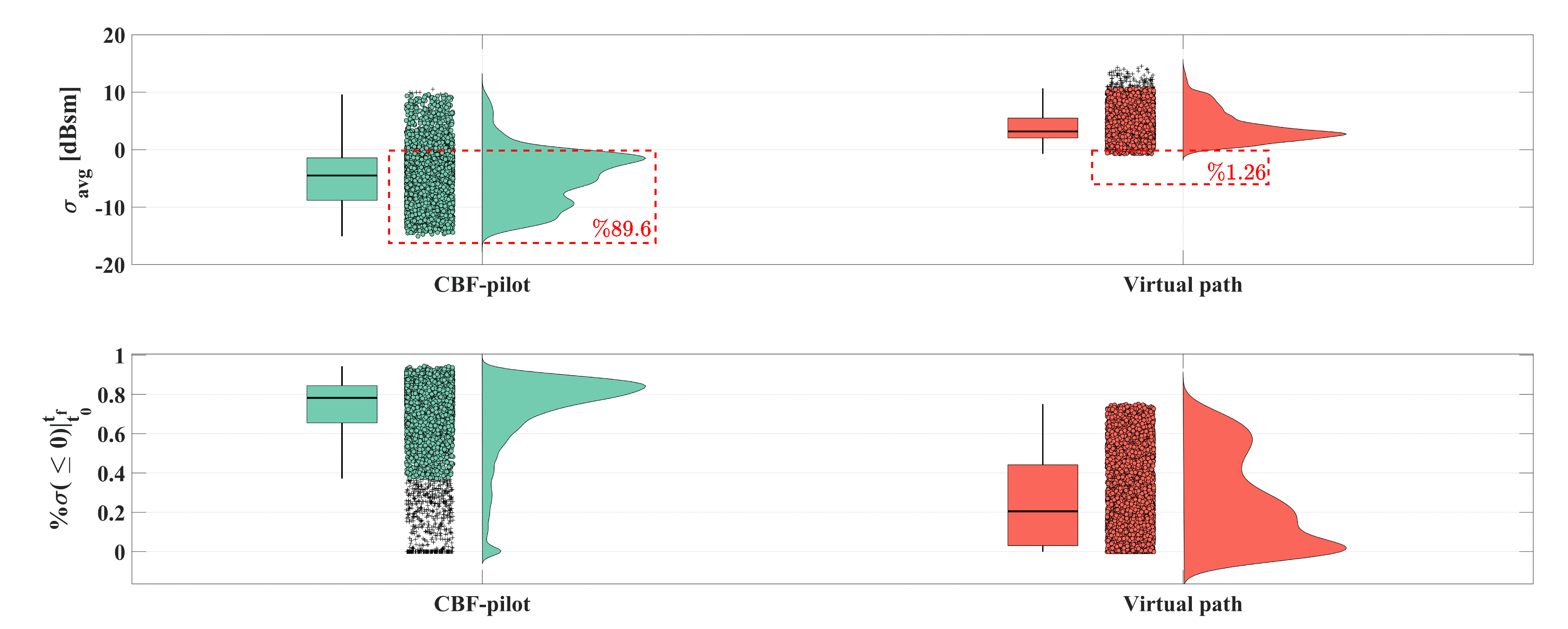
Monte Carlo simulations were employed to evaluate the performance of the proposed stealth-maneuver generation framework under varying initial conditions considering radar-penetration maneuvers, thereby simulations were terminated at the time the aircraft encounters to the radar. Each simulation was conducted under two distinct conditions: one where the RCS threshold of 0 dBsm was enforced, and another where no RCS threshold was applied . For each condition, 6355 simulations were carried out, resulting in a total of 12710 simulations. This extensive set of simulations enabled the statistical evaluation of the system’s performance. The aircraft’s altitude was randomized within the interval [1000m, 3000m], while the radar’s position was varied with its north coordinate ranging within [2000, 5000] and its east coordinate ranging within [-2000, 2000]. The performance of the framework was assessed using three key metrics as depicted in Figure 18.
The first metric, , represents the mean RCS value observed during each simulation, providing an overall measure of radar visibility. The distribution of values for both the proposed framework and the virtual path is shown in the upper portion of Figure 18. The concentration of values is below the 0 dBsm threshold for the CBF-Pilot, while it remains above the threshold for the virtual path, as expected. Additionally, the maximum values for the CBF-Pilot are smaller than those for the virtual path, reflecting the efforts to reduce visibility. The second metric focuses on the percentage of total simulations in which the mean RCS value was below the 0 dB threshold, highlighting the framework’s effectiveness in maintaining low observability across different scenarios. This metric reveals a significant difference between the results of the CBF-Pilot and the virtual path. Specifically, the virtual path achieves only of cases with below the threshold, whereas the proposed CBF-Pilot method successfully keeps of total simulations below the threshold. The third metric evaluates the percentage of RCS values that remain below 0 dB within each simulation, offering insights into the consistency of stealth performance. Relying solely on for performance measurement can be misleading, as cases where the RCS value exceeds the threshold for a certain duration can still result in an average below the threshold if the RCS achieves very low dBsm values for a short time. Therefore, using this metric provides deeper insights into the true performance. The results indicate that, for the majority of cases, the RCS value remains below the threshold for over of the total simulation time in the CBF-Pilot results. Conversely, the virtual path lacks this characteristic due to the absence of CBF constraints. These three metrics combined demonstrate the effectiveness of the proposed maneuver generation approach under various conditions and solidify its impact on reducing the aircraft’s visibility.
6. Conclusions
This study presents a novel framework for generating maneuvers using CBF to dynamically manage RCS constraints. The approach utilizes high-fidelity flight dynamics model of F16 aircraft in contrary to existing studies based on simplified kinematic flight dynamics models to assess radar observability. Additionally, the generation of the RCS dataset is made by incorporating the control surface deflections in addition to the aircraft’s orientations to realistically model the exact RCS profile. The approach allows non-stealth aircraft to reduce their radar observability by the generated maneuvers in real time, ensuring compliance with RCS thresholds.
The effectiveness of the proposed method was evaluated through comparisons between cases with CBF-pilot and virtual path which excludes CBF-based maneuver generator. In scenarios where virtual path was applied, the aircraft exhibited consistently higher RCS values, making them more susceptible to radar detection. By contrast, the CBF-pilot approach maintained RCS values below predefined thresholds for the majority of the mission timeline. In realistic operational scenarios, such as radar-penetration and radar-evasive maneuvers, the framework demonstrated its ability to dynamically adjust the aircraft’s orientation by controlling angular rates to minimize radar exposure. During Monte Carlo simulations, over of cases with stealth maneuver generator achieved sustained low radar observability, compared to just of cases with virtual path. These results underline the critical impact of dynamic and adaptive maneuver planning in achieving low detectability under radar threat conditions. This analysis illustrates the performance of the CBF-based method in enabling aircraft to evade radar detection and maintain survivability.
In conclusion, this study provides a practical and effective solution for enabling non-stealth aircraft to dynamically evade radar detection through generated maneuvers. By comparing cases with and without stealth maneuver generator, the results emphasize the importance of dynamic maneuver generation in reducing radar observability. The proposed framework sets a new benchmark for enhancing survivability in contested environments and lays the groundwork for future innovations in stealth strategy and maneuver planning. Thus, potential future work may involve assessing the framework under more challenging scenarios, such as dynamic radar threats posed by aerial radar platforms. Additionally, incorporating pilot-support algorithms, such as ground collision avoidance and flight envelope protection, could evaluate the compatibility of RCS-constrained maneuver commands with safe envelope limits and collision avoidance requirements.
Author Contributions
Conceptualization, methodology, software, writing—original draft preparation, Mustafa Demir, Ege C. Altunkaya, Akın Çatak, Fatih Erol; writing—spuervising, review and editing, Emre Koyuncu, Uğur Zengin, Íbrahim Özkol. All authors have read and agreed to the published version of the manuscript.
Funding
This research received no external funding.
Institutional Review Board Statement
Not applicable.
Data Availability Statement
Dataset available on request from the authors.
Acknowledgments
During the preparation of this manuscript/study, the author(s) used ChatGPT 4.0 for the purposes of the grammar and spell check. The authors have reviewed and edited the output and take full responsibility for the content of this publication.
Conflicts of Interest
The authors declare no conflicts of interest.
Abbreviations
The following abbreviations are used in this manuscript:
| CBF | Control barrier functions |
| INDI | Incremental nonlinear dynamic inversion |
| LO | Low-observability |
| RAM | Radar-absorbing material |
| RCS | Radar cross-section |
| UAV | Unmanned aerial vehicle |
| CAS | Control augmentation system |
References
- Paterson, J. Overview of low observable technology and its effects on combat aircraft survivability. Journal of Aircraft 1999, 36, 380–388. [Google Scholar] [CrossRef]
- Moore, F.W. Radar cross-section reduction via route planning and intelligent control. IEEE Transactions on Control Systems Technology 2002, 10, 696–700. [Google Scholar] [CrossRef]
- Zikidis, K.; Skondras, A.; Tokas, C. Low observable principles, stealth aircraft and anti-stealth technologies. Journal of Computations & Modelling 2014, 4, 129–165. [Google Scholar]
- Woo, S.H.A.; Shin, J.J.; Kim, J. Implementation and analysis of pattern propagation factor based radar model for path planning. Journal of Intelligent & Robotic Systems 2019, 96, 517–528. [Google Scholar]
- Norsell, M. Radar cross section constraints in flight-path optimization. Journal of aircraft 2003, 40, 412–415. [Google Scholar] [CrossRef]
- Zhang, Z.; Jiang, J.; Wu, J.; Zhu, X. Efficient and optimal penetration path planning for stealth unmanned aerial vehicle using minimal radar cross-section tactics and modified A-Star algorithm. ISA transactions 2023, 134, 42–57. [Google Scholar] [CrossRef]
- Guan, J.; Huang, J.; Song, L.; Lu, X. Stealth Aircraft Penetration Trajectory Planning in 3D Complex Dynamic Environment Based on Sparse A* Algorithm. Aerospace 2024, 11, 87. [Google Scholar] [CrossRef]
- Zhang, Z.; Wu, J.; Dai, J.; He, C. A novel real-time penetration path planning algorithm for stealth UAV in 3D complex dynamic environment. Ieee Access 2020, 8, 122757–122771. [Google Scholar] [CrossRef]
- Zhang, Z.; Wu, J.; Dai, J.; He, C. Rapid penetration path planning method for stealth uav in complex environment with bb threats. International Journal of Aerospace Engineering 2020, 2020, 8896357. [Google Scholar] [CrossRef]
- Guo, D.; Zhai, J.; Xie, X.; Yin, H.; Zhu, Y. Machine learning-based modeling and uncertainty quantification for radar cross section of a cone-like target. In Proceedings of the 2022 IEEE 2nd International Conference on Power, Electronics and Computer Applications (ICPECA). IEEE; 2022; pp. 249–252. [Google Scholar]
- McFarland, M.B.; Zachery, R.A.; Taylor, B.K. Motion planning for reduced observability of autonomous aerial vehicles. In Proceedings of the Proceedings of the 1999 IEEE International Conference on Control Applications (Cat. No. 99CH36328). IEEE, 1999, Vol. 1, pp. 231–235.
- Xu, Q.; Ge, J.; Yang, T.; Sun, X. A trajectory design method for coupling aircraft radar cross-section characteristics. Aerospace Science and Technology 2020, 98, 105653. [Google Scholar] [CrossRef]
- Lu, X.; Huang, J.; Guan, J.; Song, L. Stealth Aircraft Penetration Trajectory Planning in 3D Complex Dynamic Based on Radar Valley Radius and Turning Maneuver. Aerospace 2024, 11, 402. [Google Scholar] [CrossRef]
- Paterson, J. Measuring low observable technology’s effects on combat aircraft survivability. In Proceedings of the 1997 World Aviation Congress; 1997; p. 5544. [Google Scholar]
- Liu, H.; Chen, J.; Shen, L.; Chen, S. Low observability trajectory planning for stealth aircraft to evade radars tracking. Proceedings of the Institution of Mechanical Engineers, Part G: Journal of Aerospace Engineering 2014, 228, 398–410. [Google Scholar] [CrossRef]
- Liu, H.; Chen, S.; Zhang, Y.; Chen, J. Modelling radar tracking features and low observability motion planning for UCAV. In Proceedings of the 2012 4th International Conference on Intelligent Human-Machine Systems and Cybernetics. IEEE, 2012, Vol. 2, pp. 162–166.
- Nguyen, L.T. Simulator study of stall/post-stall characteristics of a fighter airplane with relaxed longitudinal static stability; Vol. 12854, National Aeronautics and Space Administration, 1979.
- Ames, A.D.; Coogan, S.; Egerstedt, M.; Notomista, G.; Sreenath, K.; Tabuada, P. Control barrier functions: Theory and applications. In Proceedings of the 2019 18th European control conference (ECC). IEEE; 2019; pp. 3420–3431. [Google Scholar] [CrossRef]
- Nguyen, Q.; Sreenath, K. Exponential control barrier functions for enforcing high relative-degree safety-critical constraints. In Proceedings of the 2016 American Control Conference (ACC). IEEE; 2016; pp. 322–328. [Google Scholar] [CrossRef]
- Pavlovic, M.S.; Tasic, M.S.; Mrdakovic, B.L.; Kolundzija, B. WIPL-D: Monostatic RCS analysis of fighter aircrafts. In Proceedings of the 2016 10th European Conference on Antennas and Propagation (EuCAP). IEEE; 2016; pp. 1–4. [Google Scholar]
Figure 1.
The illustration of a radar-penetration maneuver scenario, emphasizing the virtual (or ideal) path and alternative RCS-constrained maneuvers.
Figure 1.
The illustration of a radar-penetration maneuver scenario, emphasizing the virtual (or ideal) path and alternative RCS-constrained maneuvers.
Figure 2.
An illustration of the baseline aircraft with its body axis and wind axis frames.
Figure 3.
Digital F-16 geometry and mesh.
Figure 4.
The azimuth () and elevation () representation: the relative orientation of the aircraft with respect to the radar position.
Figure 4.
The azimuth () and elevation () representation: the relative orientation of the aircraft with respect to the radar position.
Figure 5.
F-16 RCS characteristics with the elevation, , and azimuth, : the RCS profiles indicate that the peak values are observed in the azimuth angles of and , while the elevation is constant at . Additionally, the peaks are trackable at the elevation angles of and , while the azimuth is constant at . The RCS characteristics and values at different orientations of F-16 clearly exhibit the toughness of generating stealthy maneuvers. (a) RCS variation while the elevation, , remains constant at . (b) RCS variation while the azimuth, , remains constant at .
| (a) | (b) |
Figure 6.
F-16 RCS characteristics in polar map. (a) RCS variation while the azimuth, , remains constant at . (b) RCS variation while the azimuth, , remains constant at .
Figure 6.
F-16 RCS characteristics in polar map. (a) RCS variation while the azimuth, , remains constant at . (b) RCS variation while the azimuth, , remains constant at .
| (a) | (b) |
Figure 7.
F-16 RCS variation with the horizontal tail deflection. (a) Positive horizontal tail deflection. (b) Negative horizontal tail deflection.
Figure 7.
F-16 RCS variation with the horizontal tail deflection. (a) Positive horizontal tail deflection. (b) Negative horizontal tail deflection.
| (a) | (b) |
Figure 8.
F-16 RCS variation with the rudder deflection.
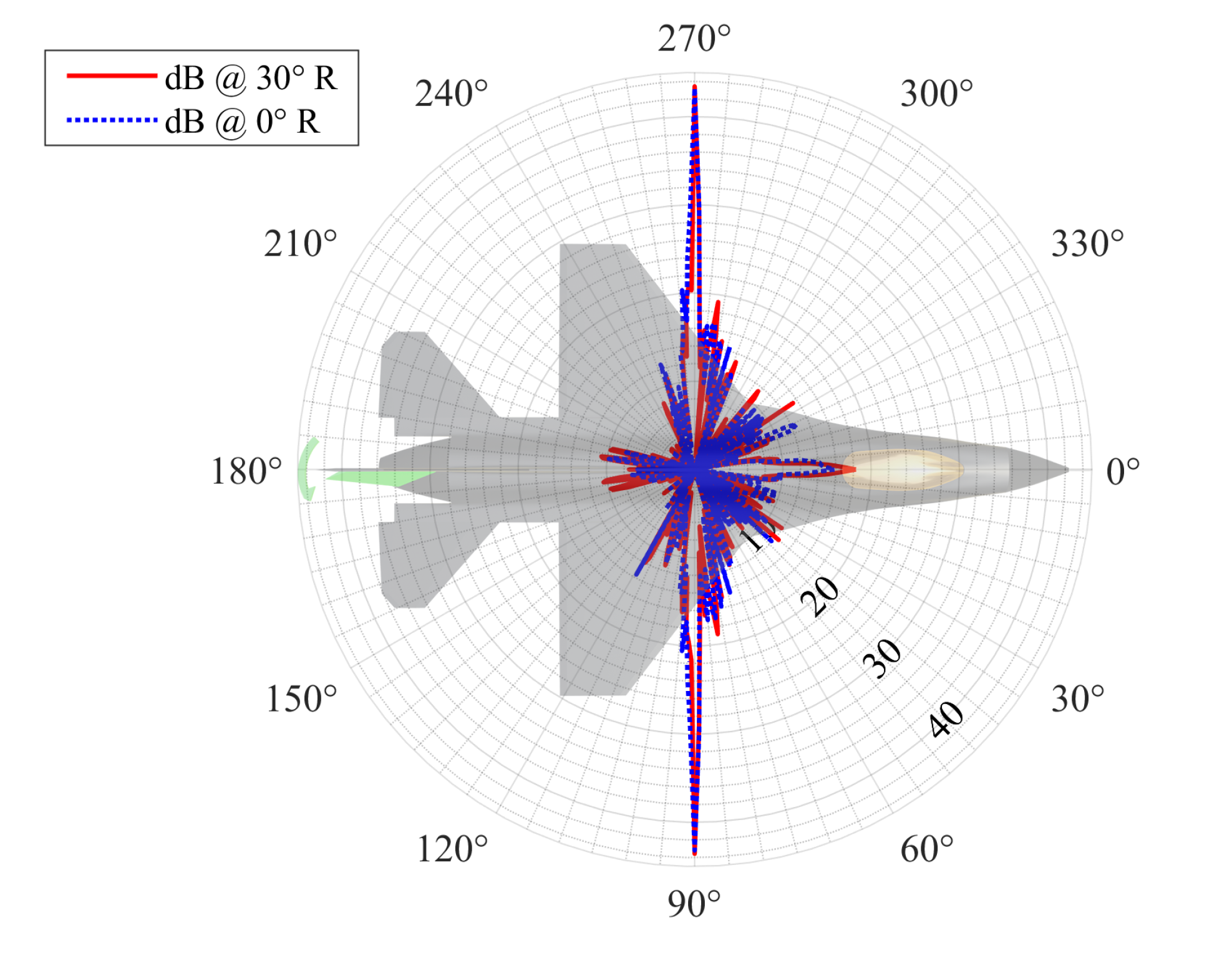
Figure 9.
General framework of the proposed method: (1) Stealth-maneuver generator through CBF-pilot, (2) CAS including INDI, and (3) A/C dynamics. The reference commands , , and from virtual path are subjected to RCS constraint. Each reference angular rate signals are adjusted by CBF constraint, and , , and are generated, if necessary. Otherwise, the reference angular rate commands are passed through.
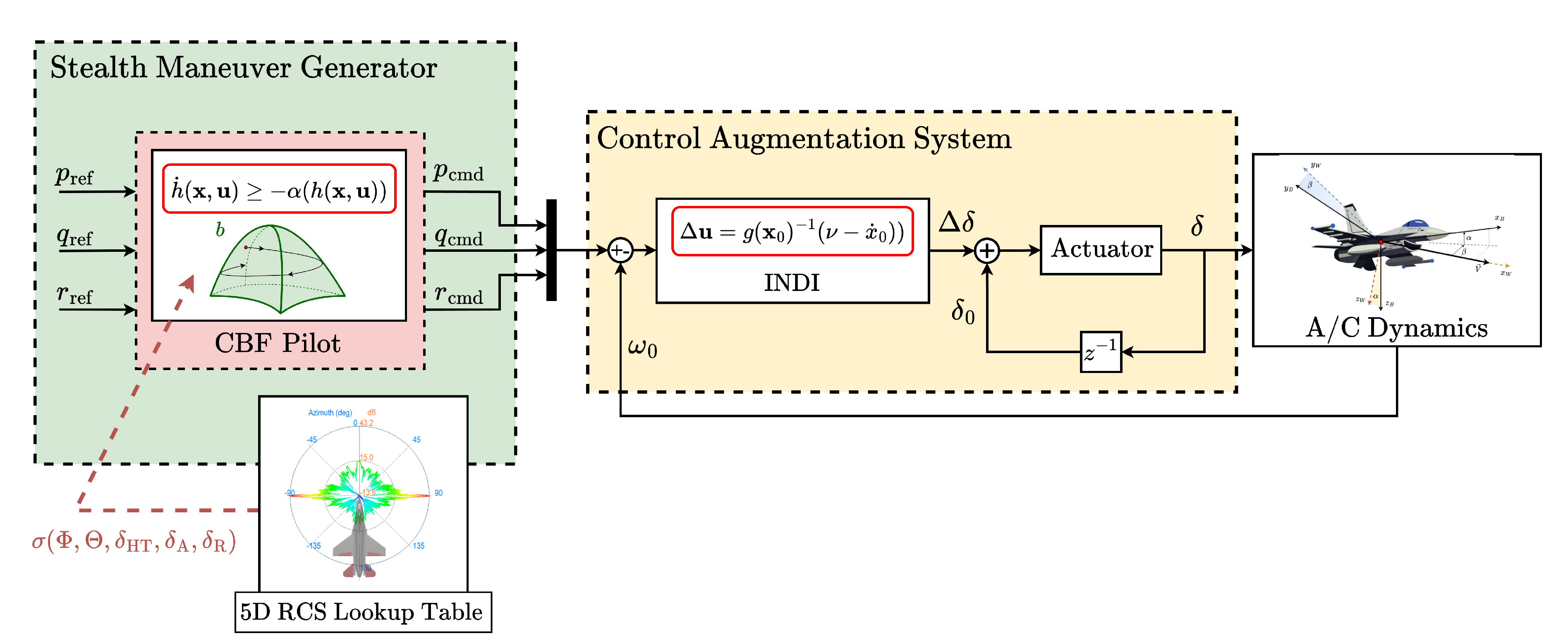
Figure 10.
Radar cross-section history for the radar-penetration maneuver: 1) RCS trajectories for both the virtual path and RCS-constrained maneuver on the left, 2) RCS map with azimuth and elevation angles, along with the aircraft’s orientation trajectory on the right.
Figure 10.
Radar cross-section history for the radar-penetration maneuver: 1) RCS trajectories for both the virtual path and RCS-constrained maneuver on the left, 2) RCS map with azimuth and elevation angles, along with the aircraft’s orientation trajectory on the right.
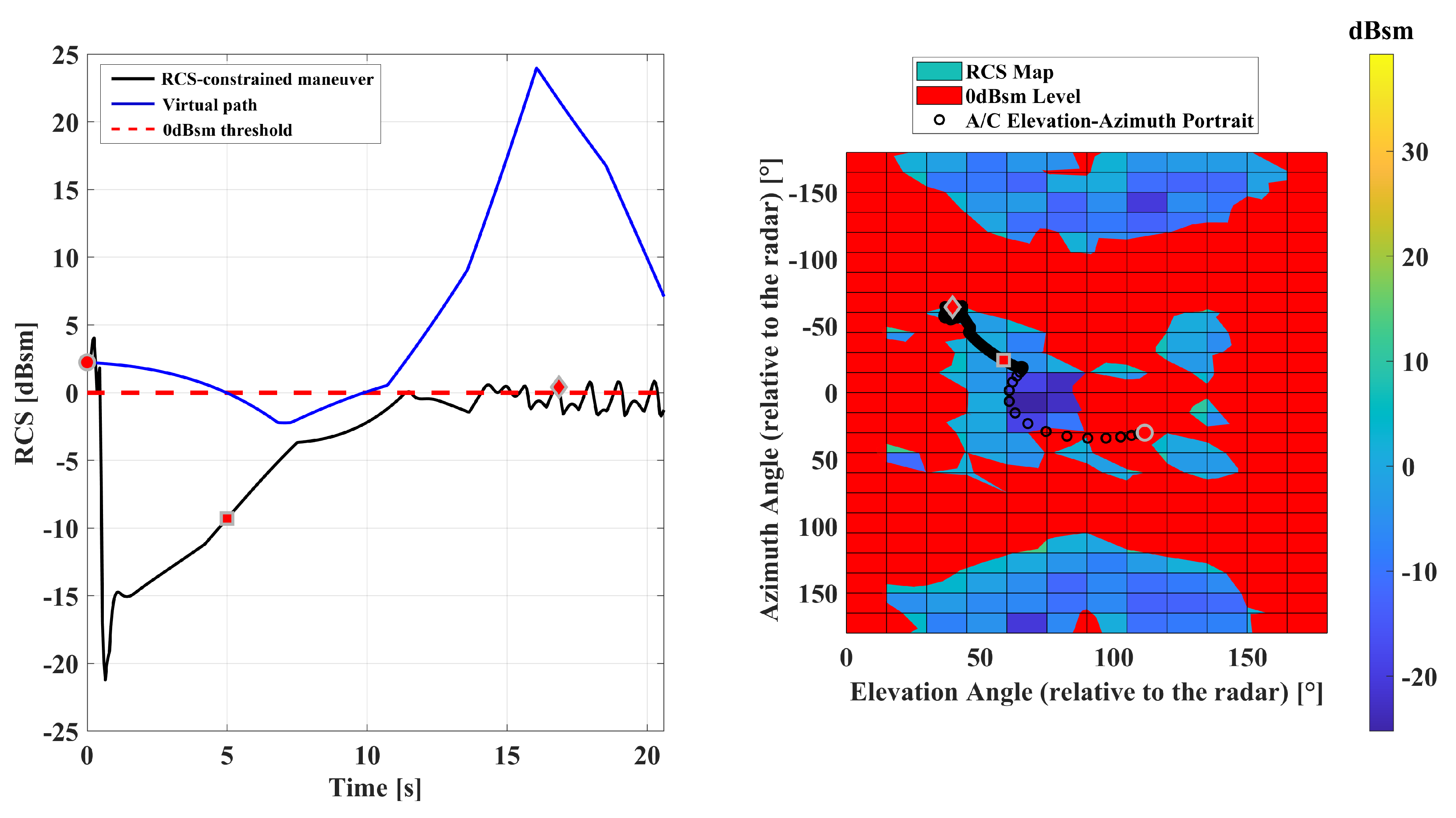
Figure 11.
CBF-pilot commands for the radar-penetration maneuver.
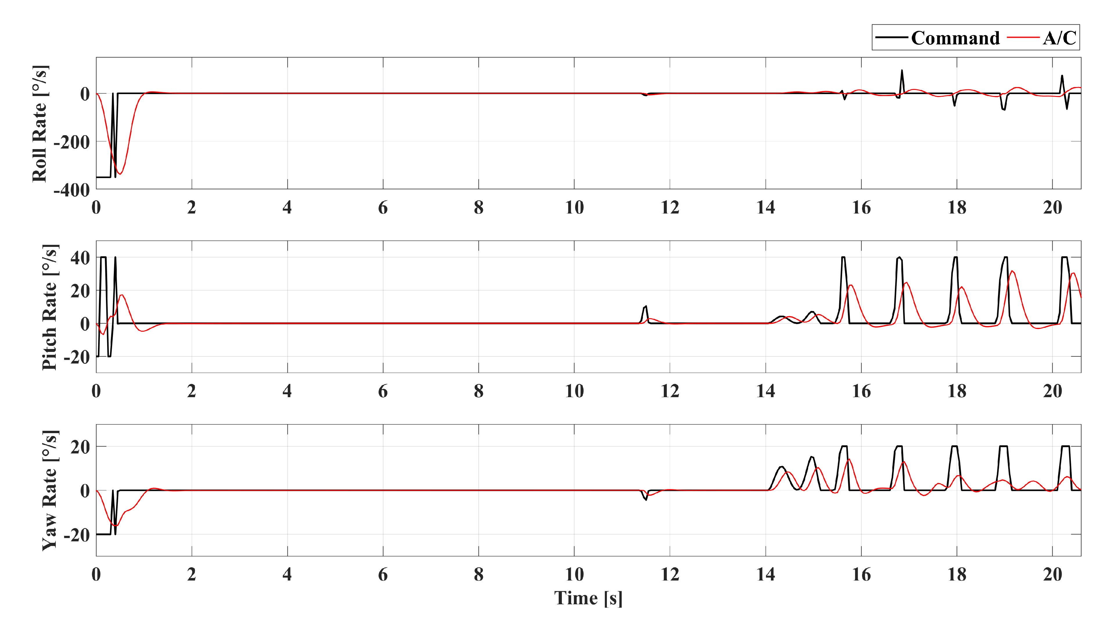
Figure 12.
Attitude trajectories of the aircraft during the radar-penetration maneuver.
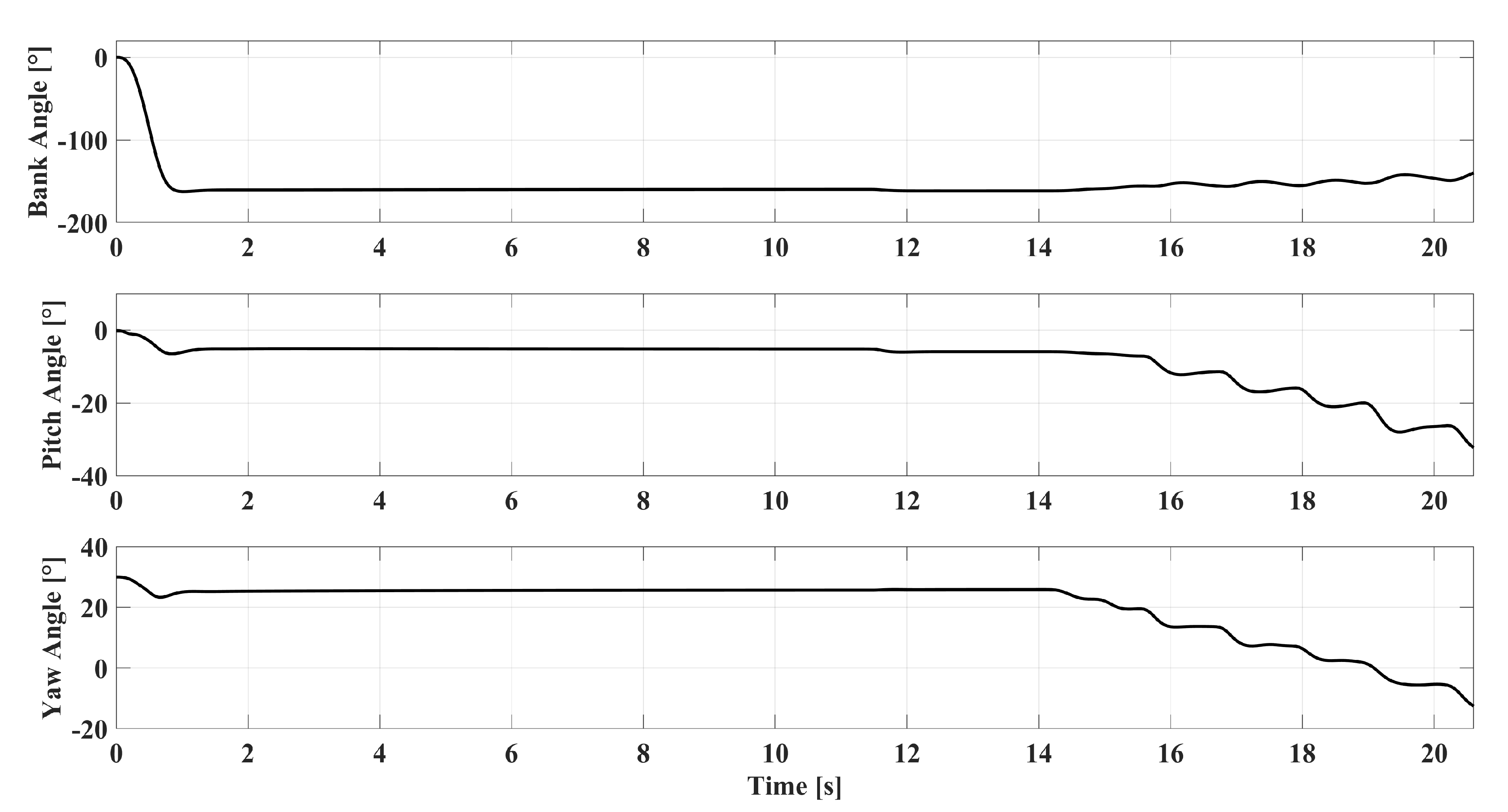
Figure 13.
3D visualization of the radar-penetration maneuver scenario.
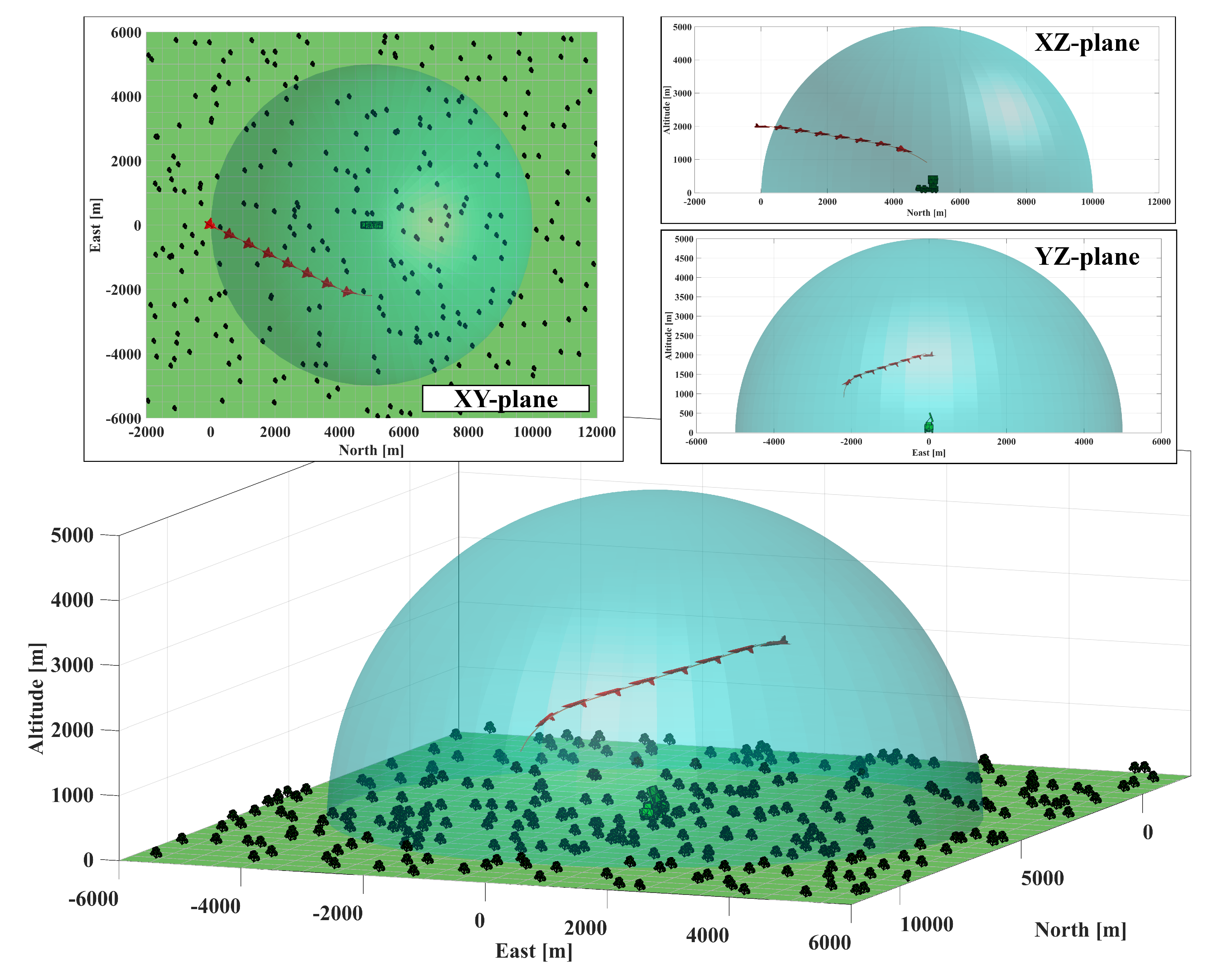
Figure 14.
Radar cross-section history for the radar-evasive maneuver: 1) RCS trajectories for both the virtual path and RCS-constrained maneuver on the left, 2) RCS map with azimuth and elevation angles, along with the aircraft’s orientation trajectory on the right.
Figure 14.
Radar cross-section history for the radar-evasive maneuver: 1) RCS trajectories for both the virtual path and RCS-constrained maneuver on the left, 2) RCS map with azimuth and elevation angles, along with the aircraft’s orientation trajectory on the right.
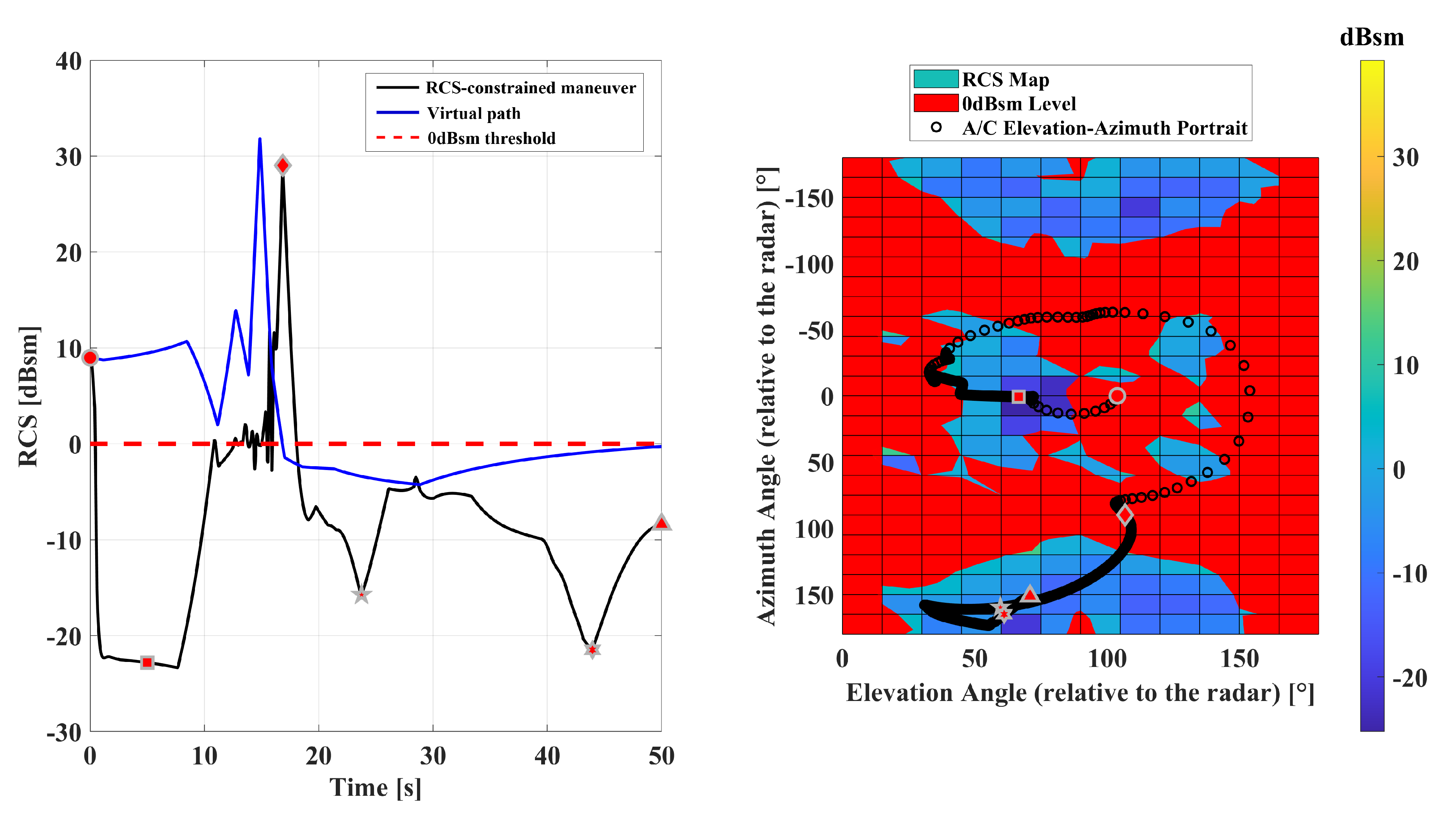
Figure 15.
CBF-pilot commands for the radar-evasive maneuver.
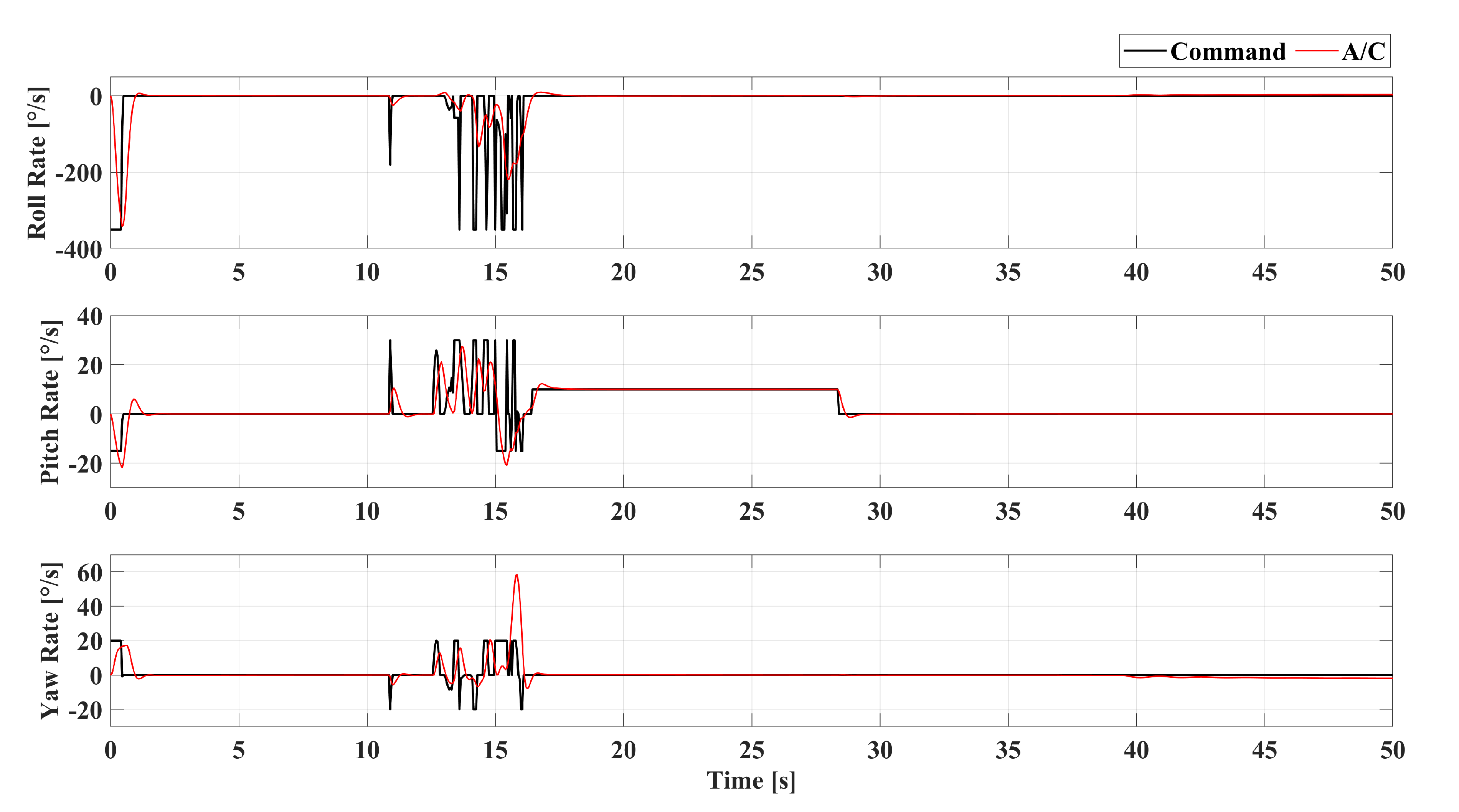
Figure 16.
Attitude trajectories of the aircraft during the radar-evasive maneuver.
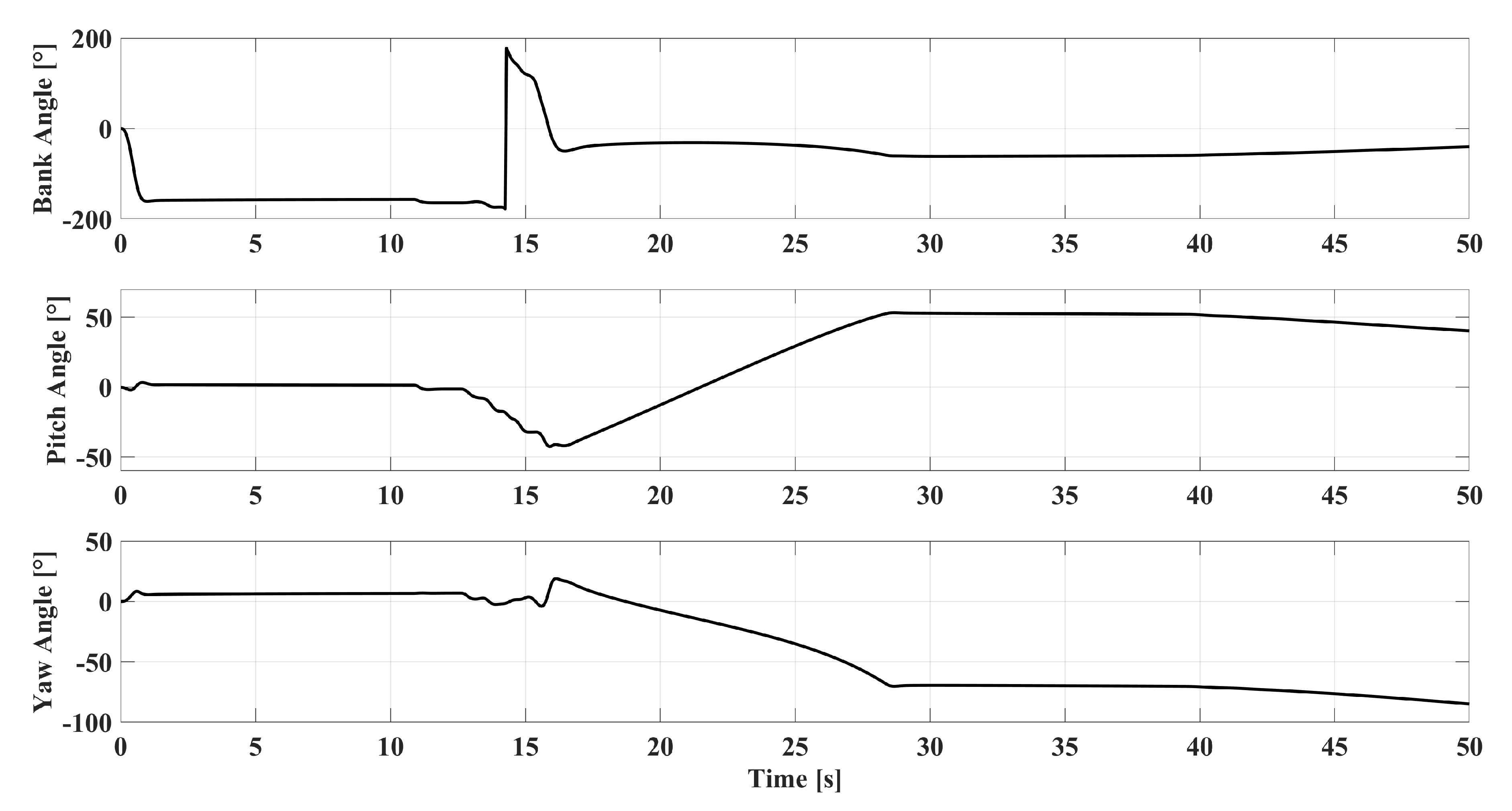
Figure 17.
3D visualization of the radar-evasive maneuver scenario.
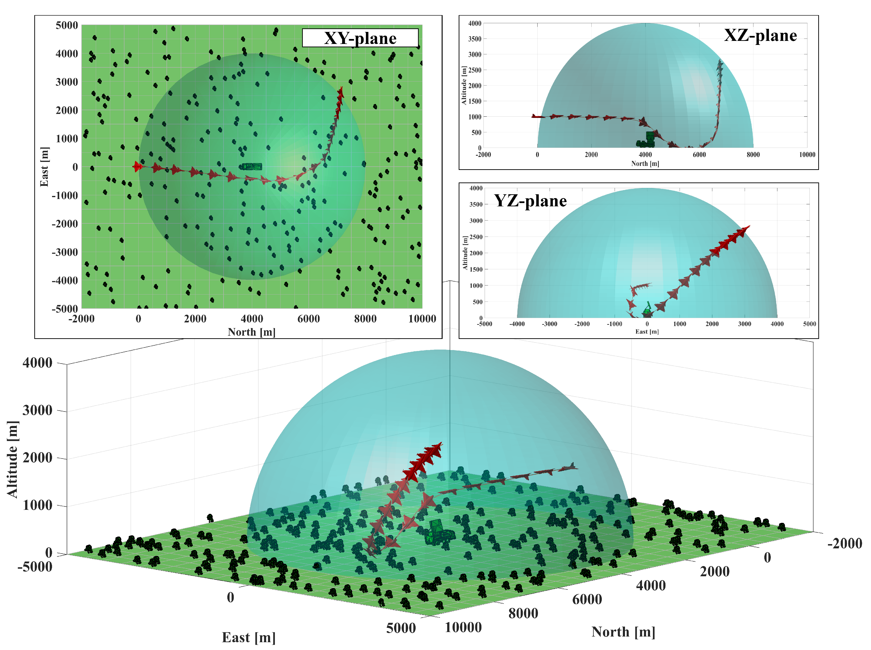
Figure 18.
Monte Carlo simulation performance metrics: 1) The mean RCS value is dBsm and dBsm for the CBF-pilot and the virtual path, respectively; 2) The percentage of the mean RCS below the threshold is for the CBF-pilot and for the virtual path; 3) The RCS value remains below the threshold for and of the simulation duration for the CBF-pilot and the virtual path, respectively.
Disclaimer/Publisher’s Note: The statements, opinions and data contained in all publications are solely those of the individual author(s) and contributor(s) and not of MDPI and/or the editor(s). MDPI and/or the editor(s) disclaim responsibility for any injury to people or property resulting from any ideas, methods, instructions or products referred to in the content. |
© 2025 by the authors. Licensee MDPI, Basel, Switzerland. This article is an open access article distributed under the terms and conditions of the Creative Commons Attribution (CC BY) license (http://creativecommons.org/licenses/by/4.0/).
Copyright: This open access article is published under a Creative Commons CC BY 4.0 license, which permit the free download, distribution, and reuse, provided that the author and preprint are cited in any reuse.


