
Submitted:
02 January 2025
Posted:
06 January 2025
You are already at the latest version
Abstract
Given the considerable length and weight of freight trains, their operation can be quite challenging. Improper operation may lead to train decoupling and derailment. Driver Advisory Systems (DASs) are used in some countries to assist the train drivers by providing the speed curves, which are desired to be easy to track. Multi-mass train model is a good choice to depict the in-train forces in train speed curve generating, but its application is often hindered by the computation time. Single mass train model is considered as another choice to simplify the computation. To exploit the advantages of the multi-mass and single mass models, this paper proposes a Two-step Optimization Method to generate the optimal speed curves for the freight trains. In the first step, the Rolling Optimization Algorithm (ROA) is proposed to optimize the speed curve on the basis of single mass model, taking the train energy consumption and punctuality as the optimization objectives. In order to assist the driver to operate the train smoothly, the speed curve generated by the ROA was tested on DAS, but it could not be followed accurately in actual operation. To solve this problem, a Model Predictive Control (MPC) algorithm based on multi-mass model is adopted as the second optimization step, which takes the output speed curve of the ROA as the reference speed curve. The MPC algorithm will generate a new speed curve, taking in-train forces, energy consumption and punctuality as the optimization indices. Simulations are carried out using the data of Dalailong railway in China to evaluate the proposed method. The simulation results show that the speed curves generated by Two-step Optimization Method are smoother than that of the ROA, and the throttle sequences are more conducive for the driver to follow in practical operation. The simulation results show that the energy consumption is reduced by 17.1% compared to that of ROA simulation. The speed curve also can be integrated into the onboard DAS or the Automatic Train Operation (ATO) system, aiming to obtain a smooth and energy-efficient train operation.
Keywords:
MPC
; Rolling Optimization
; Train Operation Optimization
; Energy Saving
1. Introduction
In recent years, the freight transportation has quickly increased [1]. As the freight trains are heavy and long, it is difficult to operate the freight trains smoothly. If the longitudinal impulse is too big, it will shorten the life of train couplers, and even cause fatal accidents such as coupler breakdown and derailment. The operation strategies also influence the train energy consumption. Due to the differences of driving skills and experience of the drivers, the train energy consumption is also different. Even for the same driver, the train operation is also affected by his state, physical and mental, operating conditions, line conditions, and the train condition. Therefore, it is necessary to improve the train operation by providing a smooth and energy-efficient train speed curve, which can be integrated into the Driver Advisory System (DAS) or Automatic Train Operation (ATO) system.
When optimizing the train speed curve, establishing a train dynamic model is an essential step. Single mass model and multi-mass model are both widely studied by scholars. The single mass model is characterized by its comparatively fast computation speed. Howlett used the single mass model to investigate the energy-efficient train control method [2]. Based on the single mass model, Howlett used a new local energy minimization principle to calculate the optimal switching points with steep gradients [3]. Pudovikov simulated the train operation dynamic processes to improve the control effect of the automatic control system for freight train speeds [4]. The single mass model cannot depict the in-train force, while the multi-mass model can consider the in-train force. Consequently, the optimization outputs based on multi-mass model are more applicable to the real-word situation. Gruber introduced the concept of multi-mass model by studying the problem of optimizing the heavy trains towed by multiple locomotives [5]. Chou conducted an optimal control study for the energy saving and speed tracking problems using the LQR (Linear Quadratic Regulator) methodology based on the validated multi-mass model [6]. Zhuan proposed an output regulation method with measurement feedback control of heavy-duty trains based on the multi-mass model, controlling the train speed within a specified speed range [7].
The train speed curves are initially optimized by Pontryagin maximum principle rules and other algorithms. Howlett provided the key equations for optimal control strategies with minimum energy consumption and punctual operation under continuously changing gradients [8]. Khmelnitsky investigated the problem of train energy-saving operation under arbitrary changes of speed and gradient, and realized the corresponding energy-saving control strategy in this context [9]. Martinis proposed a method for generating energy-saving speed curves for freight trains by analyzing data from a real-time vehicle monitoring system [10]. Ko used a dynamic programming method to generate energy-efficient train operating speed curves, and reduced the computation time and speed errors by improving the dynamic programming method [11]. Albrecht proposed a two-layer optimization algorithm, which is able to compute and generate a sequence of energy-saving optimization operations for trains with a minimum number of condition transitions [12]. Guo used the particle swarm algorithm and the NSGA-II (Non-dominated Sorting Genetic Algorithm-II) algorithm to propose a multi-objective optimization algorithm based on the energy consumption and the running time [13]. Yi used the greedy algorithm and improved multi-objective bald eagle search algorithm to solve a multi-objective optimization problem for freight trains [14]. Yang designed a fuzzy adaptive genetic algorithm (FAGA) for multi-objective curve optimization strategy, and used the improved high-order model-free adaptive iterative learning control algorithm to track the optimized speed curve [15].
There are many methods that can be used in freight train control to track the reference speed curve, in which the Model Predictive Control Algorithm considering the train multi-mass model is widely used in solving the train control problem. The MPC algorithm can also be seen as a short-distance optimization method for the train speed curve. Isna Silvia applied the MPC method to predict and adjust the dwell time and the running time of the train [16]. Song designed a constrained MPC closed-loop control algorithm, customized the target curve acting on the MPC according to the operating conditions of the loaded train [17]. Liu solved the optimal control problem based on the MPC framework under the constraints of operating conditions, and analyzed the impact of different weight factors. The simulation results of MPC are compared with fuzzy control and PID (Proportion Integration Differentiation) control, and verified the feasibility of the model predictive controller [18]. A nonlinear MPC algorithm is proposed to optimize train adhesion control by identifying the trajectory parameters online using a dynamic forgetting factor recursive least squares method, and then these parameters are applied to the MPC to achieve optimal adhesion control [19]. In order to solve the optimal operation of heavy-duty trains, the MPC method was used to optimize train performance and operation through the analysis of various penalty factors, weight coefficients, etc., and the MPC reference speed are self-setting step-type curves [20,21,22,23]. The above studies on MPC algorithms usually use a step curve to test the control performance, and it is possible to optimize the train operation by taking advantage of the MPC algorithm. MPC can only be used in short term optimization of the freight train speed curve.
To leverage the advantages of the single mass model and multi-mass model, a Two-Step Optimization Method is proposed in this paper. Firstly, using ROA to generate a speed curve based on a single mass model. Secondly, inspired by the MPC control method, the paper will use the MPC method to re-optimize the train speed curve based on the multi-mass model.
2. The Two-Step Optimization Method
In this paper, a Two-Step Optimization Method is adopted to optimize the freight train speed curve, and the framework of the proposed algorithm is shown in Figure 1. ROA is designed based on the previous work of our group [24], which is on the basis of the single mass model. In this algorithm, the length and weight of the train are taken into account to equalize the values of the line gradient according to the gradient equivalence method. The optimization index includes the train running time and energy consumption.
2.1. Gradient Equivalent Method
When the single mass model is used in the freight train simulation, the gradient resistance force will change suddenly at the slope changing positions. Therefore, a gradient equivalence method is proposed, taking the length and weight of the train into account. Assume that the weight of the train is uniformly distributed along the length of the train, and the train slope resistance is distributed along the length of the train.
Define the equivalent gradient when the position of the train head is x, which can be calculated by
where n is the number of all locomotive/wagon in the whole train, is the weight of the kth locomotive/wagon, is the length of the kth locomotive/wagon, is the original gradient value where the kth locomotive/wagon is located, L is the total length of the train, and M is the total weight of the train. A gradient comparison is given by Figure 2, where the sub-figure above gives the original gradient and the sub-figure below gives the equivalent gradient of a demo line.
When the cruising speed is given, the line gradients can be classified into four types as shown in Table 1, where is defined as the gradient on which the train can keep the cruise speed with maximum traction force. Similarly, is defined as the gradient on which the train can keep the cruise speed with maximum braking force. Since there is no steep downhill section in the selected simulation line, it will not be discussed in the subsequent research.
According to Equation (1), calculate the equivalent gradient at each position and combine the successive gradients with the same type as a equivalent slope. The equivalent slopes of the line can be obtained as Figure 3. In order to find the optimal operation solution, set three slopes as a group, six slope combinations can be obtained as [a b a], [a c a], [b a c], [b a b], [c a b], [c a c]. As can be seen from the Figure 3, the slope combinations include [a b a], [b a c], [a c a].
2.2. Rolling Optimization Algorithm (ROA) for Freight Train Speed Curve
A Rolling Optimization Algorithm is proposed to find the optimal freight train speed curve. The flowchart of the rolling optimization algorithm is shown in Figure 4. The cruise speed is calculated according to the train information, and the switching points of the optimal operation strategies are optimized by the bisection method. Based on each cruise speed, the speed curve is calculated in a rolling strategy. Firstly, equivalent gradients of the line are calculated by Equation (1). Secondly, take three gradients as a group in each rolling step and calculate the optimal operation strategies according to the optimization rules. Roll forward to the next three gradients to continue the calculation, and stop the process until reaching the end of the line.
2.2.1. Train Speed Curve Optimization for Each Gradient Group
The ROA takes punctuality and energy saving as the optimization objectives, and establishes the optimization objective function as shown in
where is the simulated train running time in the section, is the planned running time in the section, is the energy consumption of the train running in the section , is the starting point of the current train operating section, is the end point of the current train operating section, and are the weights of the objective function, N is the slope combination number.
Considering the time constraints and throttle constraints of the train during operation, the constraint analysis is given. Regarding the time constraints, the optimized train running time will have a certain error with the planned running time. Define the maximum deviation value as , and then the section running time constraints shown in (3). In this way, the whole process running time constraints can also be defined as
where is the maximum error value of the whole running time.
Regarding the throttle constraints, it can be expressed by:
where G is the current throttle of the train, is the maximum throttle that the train is allowed, is the minimum throttle that the train is allowed.
Therefore, the optimization objective function and constraints of the ROA are as follows:
The main optimization rules of the ROA are given as follows. When a train enters an uphill section, it will search for an optimal switching point of the traction condition in advance. So that when the train pulls out of the uphill section, the running speed will not be much lower than the cruise speed. When a train enters a downhill section, it will search for an optimal switching point of the coast condition in advance. So that when the train pulls out of the downhill section, the running speed will not be much higher than the cruise speed. The comparison of different traction switching points for the uphill section are shown in the Figure 5. The comparison of different coast switching points for the downhill section are shown in the Figure 6. The is the limit speed.
Combined with the optimization objective function, there exists an optimal position of the switching point, which makes the objective function minimum. Therefore, the trisection method is used to find the optimal position of switching points in uphill and downhill sections, and the specific steps are as follows.
Step 1: Set the boundaries of the switching point as the start and end points of the gentle gradient section. Calculate the corresponding objective functions of the switching point boundaries.
Step 2: Divide into three equal parts and compute two trisections and , where is close to and is close to . Calculate the corresponding objective function values and .
Step 3: If , update the left array boundary to according to the (6). If , update the right array boundary to according to the (7).
Step 4: Repeat the above steps, and each step will narrow the interval down to two-thirds of its original length, until find the optimal switching point.
2.2.2. Speed Curves Connecting Method
According to the gradient equivalence method, combining three continuous slopes as a group. The ROA is carried out on the basis of this combination to obtain the speed curve of each group. And then the optimized speed curves are connected to obtain the train running speed curve of the whole line. Figure 7 is the speed curves rolling connecting method of some groups.
2.2.3. Cruise Speed Updating Method
Firstly, the initial cruise speed is calculated based on the start and end points of the train section and the planned running time, the calculation formula is shown in
where is the planned running time in the whole train operating line, is the starting point of the whole train operating line, is the end point of the whole train operating line.
When the optimized train running time does not satisfy the running time constraints, the cruise speed needs to be adjusted with the following rule:
Step 1: Given the difference threshold between the optimized train running time and the planned running time, compare the and in the section, where is the simulation running time of the whole train operating line, and let . If , the running time constraint is satisfied, and then the optimization is finished; Otherwise, the cruise speed needs to be adjusted and re-optimized.
Step 2: Obtain the adjustment value of cruise speed according to
Step 3: When adjusting the speed of the cruise, if , which indicates that the current cruise speed is comparatively low and the train is running slow, so let . If , which indicates that the the current cruise speed is comparatively high and the train is running faster, then let . Where is the adjusted cruise speed.
Step 4: Use the to re-optimize the speed curve until the running time constraint is satisfied.
2.3. MPC Algorithm for Freight Train Speed Curve Re-Optimization
The principle of the MPC algorithm can be specifically described as follows. At each sampling moment, an open-loop optimization problem is solved in real time for a finite period of time based on the current system state information. Then, the first few groups of data in the generated control sequence are applied to the controlled model as the control output. At the next sample moment, the optimization problem is solved again using the updated system state information as the initial condition to predict the future state of the system repeatedly [25]. Thus, the main advantage of the MPC algorithm is that it balances the effects of ideal optimization and practical uncertainty on the future finite time horizon, because the rolling optimization strategies that always establishes new optimization objectives on a practical basis. This is more practical and effective than the traditional optimal control established under ideal conditions. The principle of the MPC algorithm is shown in Figure 8.
2.3.1. The Multi-Mass Train Model
The multi-mass model takes into account not only the length of the train but also the coupler force, as shown in Figure 9. The coupler force is a direct index for evaluating the longitudinal impulse. For long-distance (heavy-duty) freight trains, the operation regulation recommends that the maximum coupler pulling force should be less than 2000 kN, and the maximum coupler pressing force should be less than 2250 kN [26]. The subsequent constraints on the coupler force will consider this recommendation.
The coupler can be regarded as a spring with damping characteristics, and then the coupler force is calculated by
where and are the coefficients related to the elastic and damping force of the coupler, and are the displacement and speed of the ith locomotive/wagon respectively, is the distance of two neighboring couplers when they are in nature state. In the subsequent calculations, we only consider the elastic force to simplify the simulation. Based on the multi-mass model, the force analysis for a single locomotive/wagon is shown in Figure 10.
For the ith locomotive/wagon, is the traction or braking force, is the front coupler force, is the latter coupler force, and is the mass of the ith locomotive/wagon.
For the first locomotive, it has no coupler force in front of it, and for the last wagon, it has no coupler force behind it. Based on the force analysis of the locomotive and wagons, the whole train motion equation is defined by
where is the total resistance force of the ith locomotive/wagon, which is
where is the additional resistance on slopes. The basic resistance force is defend by
In order to facilitate the subsequent design of the control algorithm, the train multi-mass model is simplified. Considering the train basic resistance force and unit slope additional resistance force , define and . Define as the state vectors and as the decision vectors, and then the state equation of the linearized system is
where
The model after linearization is discretized in the subsequent simulation application, and the discretized model can be expressed as
2.3.2. MPC Framework
According to the state Equation (15) of the multi-mass model of the freight train, assuming that the train operation state variable is measurable at the moment , the derivation of the state equation leads to the predicted state variable is calculated as follows:
Generalizing the above equation yields
where
where X is the train state at each predicted moment, U is the corresponding control input, and G, are the coefficient matrices. The predicted state X can be predicted by (17), and the control sequence U within the prediction range can be obtained.
2.3.3. Optimization Objective Function
In freight train operation, energy saving, punctuality and coupler force are the key factors to ensure the safe operation of the train, the operation optimization objective function of the freight train is constructed by
where is the reference speed, , , are the weighting coefficients for the coupler force, energy consumption and speed tracking error respectively, and , represent the start and end time of prediction period respectively.
and are related to the reference velocity , which is determined based on the train position, while depends on the train position and speed, so a computational method for handling these variables based on the train position and speed is given. Firstly, the speed in the predicted state is denoted as , and the position of the train at the sample moment is denoted as . Then the position of the train at the sample moment can be expressed as
where T is the sample time.
From the above equation, the predictions of and can be expressed respectively as a function of s by
Therefore, the train operation optimization objective function under the MPC framework can be expressed as
where
2.3.4. Train Operational Constraints
The freight train operation should consider the constraints of the coupler force, the traction and braking force of the locomotive. Therefore, the constraints of the freight train are given as follows:
where is the kth locomotive/wagon coupler force, and are lower and upper bounds of coupler force, is the ith traction and braking force of locomotive/wagon, and are lower and upper bounds of ith traction and braking force of locomotive/wagon.
The above constraints can be expressed in terms of state quantities:
, and , are upper and lower bounds of and U respectively.
Firstly, according to the calculation method of train coupler force, a matrix Z is constructed to extract the relative displacement between neighboring compartments in the state variable, where , Then . Secondly, according to the derivation process in (16), the same reasoning can be used to express the calculation of the coupler force as
where
Thus, the constraints on the coupler force can be expressed as follows:
3. Simulation Results
The simulation data in this paper, such as gradient and speed limit, are all the actual data of Dalailong railway in China. The simulated train is composed of a diesel locomotive and 42 C80 wagons, with a total length of 525.1 m and a total weight of 4338 t. Part of the railway from Longkougang Station to Changyibei Station is considered in the simulation, with a length of 133.4 km. This simulation was performed in Matlab.
Table 2 gives the train operation results of the MPC algorithm with different objective function weighting coefficients, while the prediction step and optimization step of the MPC algorithm are fixed when changing the weighting coefficients of the objective function. In the Table 2, and denote the maximum pulling coupler force and the maximum pressing coupler force for all locomotive/wagon during simulation, respectively, and denotes the operation time difference between the MPC algorithm and the ROA. Figure 11 and Figure 12 give the maximum pulling coupler force and the maximum pressing coupler force for all locomotive/wagon during simulation with different weighting coefficients. When = 0.1, = 10, = 10000, is 20 s, the maximum pulling and pressing coupler forces are within the recommended range, and the train speed is within the limit. Concurrently, the maximum pulling and pressing coupler forces, under the other objective function weighting coefficients, fall within the recommended limits.
Figure 13 and Figure 14 give the Two-step Optimization Method simulation speed curves for different values of and when = 10, = 6 and = 1. As can be seen from Figure 13, the simulation speed curves with different objective function weighting coefficients have little change, and the speed curves are smoother compared to the ROA simulation curve. From Figure 14, it can be seen that when the train is operated through the speed limit section, none of them exceeds the speed limit value. The coupler force becomes larger as decreases or increases.
Table 3 gives the train operation results of the MPC algorithm with different prediction step() and optimization step(), when the weight coefficients of the objective function are fixed to = 0.1, = 10, = 10000. Figure 15 gives the maximum pulling coupler force and the maximum pressing coupler force for all locomotive/wagon during simulation with different and . The optimization result is = 6, = 1.
Figure 16 and Figure 17 give the Two-step Optimization Method simulation speed curves for different values of and when = 0.1, = 10, = 10000. From Figure 16, it can be seen that when the values of and are changed, there are some differences in the generated speed curves, but they are smoother compared to the ROA simulation curve. And it can be seen from Figure 17 that when the train is operated through the speed limit section, the speed limit value is not exceeded whatever the values of and . When changing the value of and , the train speed curves change obviously, while the change in coupler force is not significant. When increases from 3 to 6 with fixed , the simulation speed curves closer to ROA simulation curve and more in line with speed limits. Meanwhile, with the decrease of while the is fixed, the simulation speed gradually changes towards the speed limit range, and when = 6, = 1 the simulation results achieve the reasonable performance. Therefore, the train will have better operation with longer prediction step and shorter optimization step.
Summarizing the above simulation results, when = 0.1, = 10, = 10000, = 6 and = 1, the maximum pulling coupler force is 34.4% of the pulling coupler force limit value, and the maximum pressing coupler force is 35.7% of the pressing coupler force limit value. It can be shown that the optimized train operation is smoother.
Figure 16.
Simulation speed curves with different and
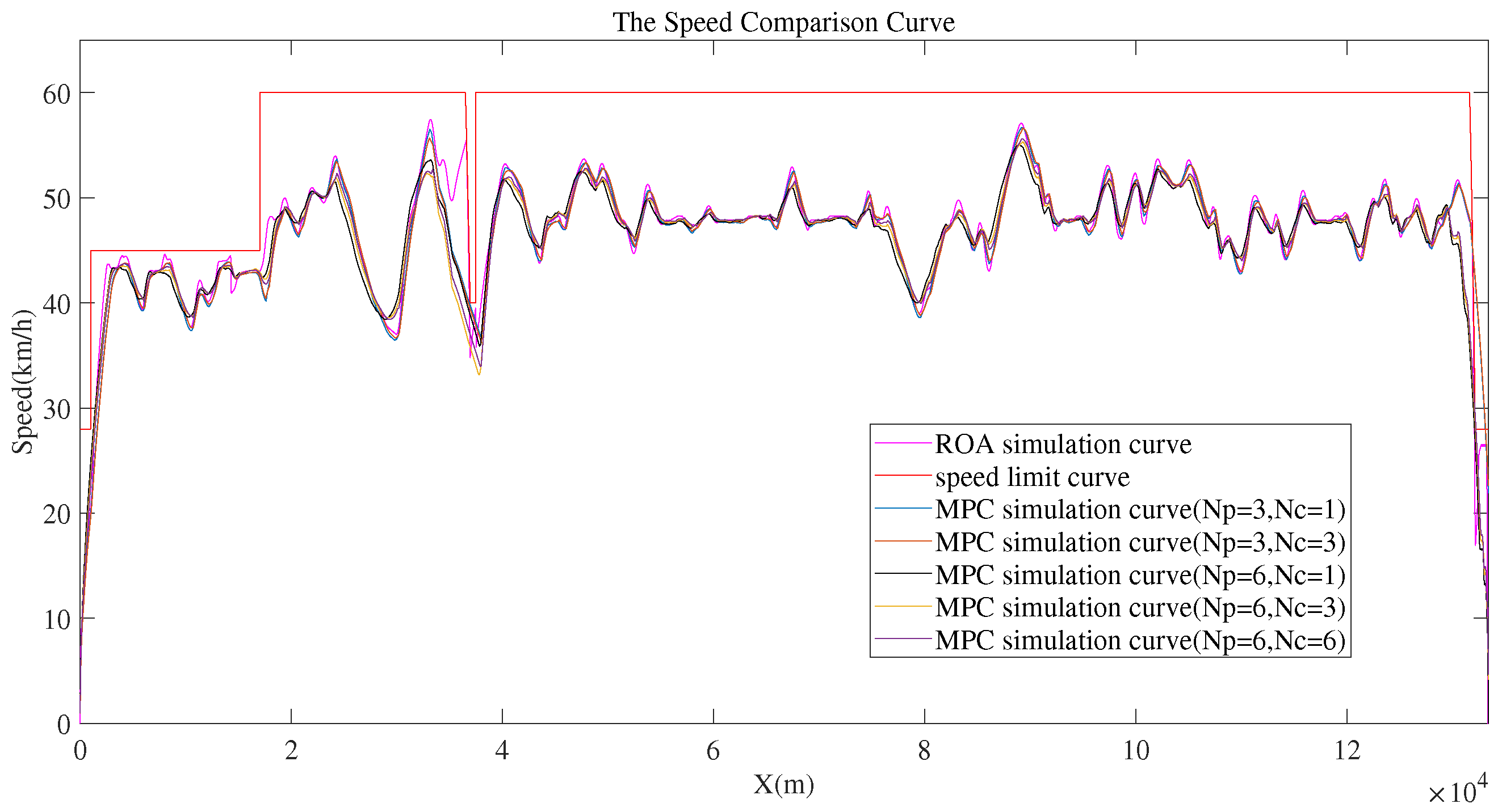
Figure 17.
Partially enlarged simulation speed curves with different and
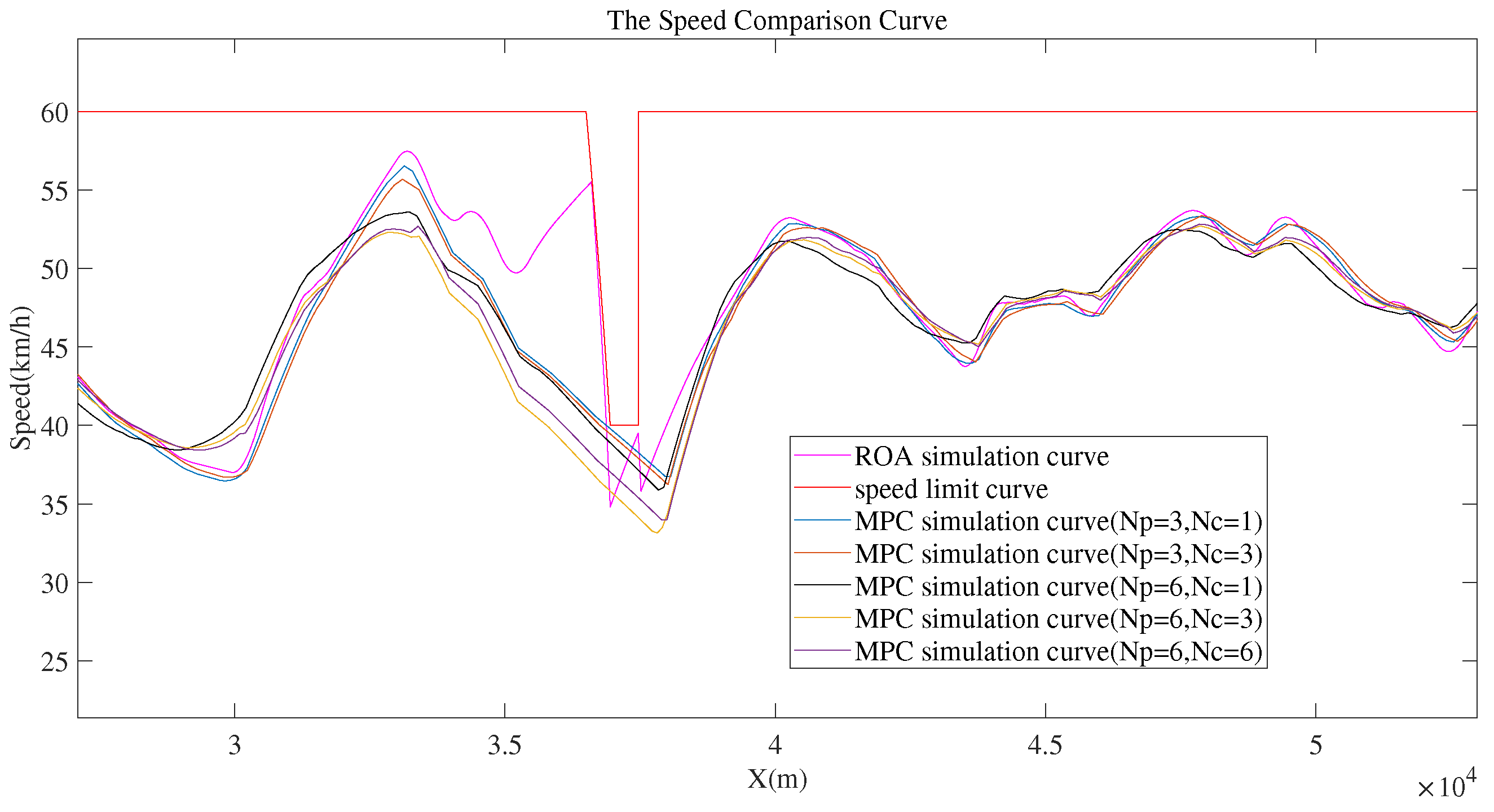
Figure 18 gives the simulation results when = 0.1, = 10, = 10000, = 6 and = 1. In the first subfigure, the red line is the speed limit curve, the purple line is the reference speed curve, the green line is the actual speed curve, and the black line is the simulation curve of MPC algorithm. The actual speed curve is plotted from the data in the LKJ(Train Operation Monitoring Equipment). In the second subfigure, the blue line represents the maximum pulling coupler force and the red line represents the maximum pressing coupler force in all locomotive/wagons at each sampling time. The third subfigure represents the line gradient curve. The horizontal coordinate indicates the distance. From the first subfigure, it can be seen that the speed curve obtained from the Two-step Optimization Method has a smaller range of speed fluctuations and is smoother. In the second subfigure, the coupler force variations of the MPC method are small and within safe limits.
Figure 19 gives the simulation results of train control strategy. The first subfigure represents the train control strategy of the MPC algorithm. The second subfigure represents that of the Rolling Optimization Algorithm. The third subfigure represents the gradient curve. The vertical coordinate values in the first two subfigures represent the throttles, where means that the train has neither traction nor braking force, means that the train is in traction, and means that the train is braking. The horizontal coordinate indicates the distance. It can be seen that the control strategies generated by the MPC algorithm and the Rolling Optimization Algorithm are similar, and when the train travels between 60 km and 72 km, the throttles generated by the MPC algorithm change less. Hence, the control strategy generated after the Two-step Optimization Method is easier to follow for the drivers during actual operation.
Figure 18.
Train speed curves and coupler force comparisons
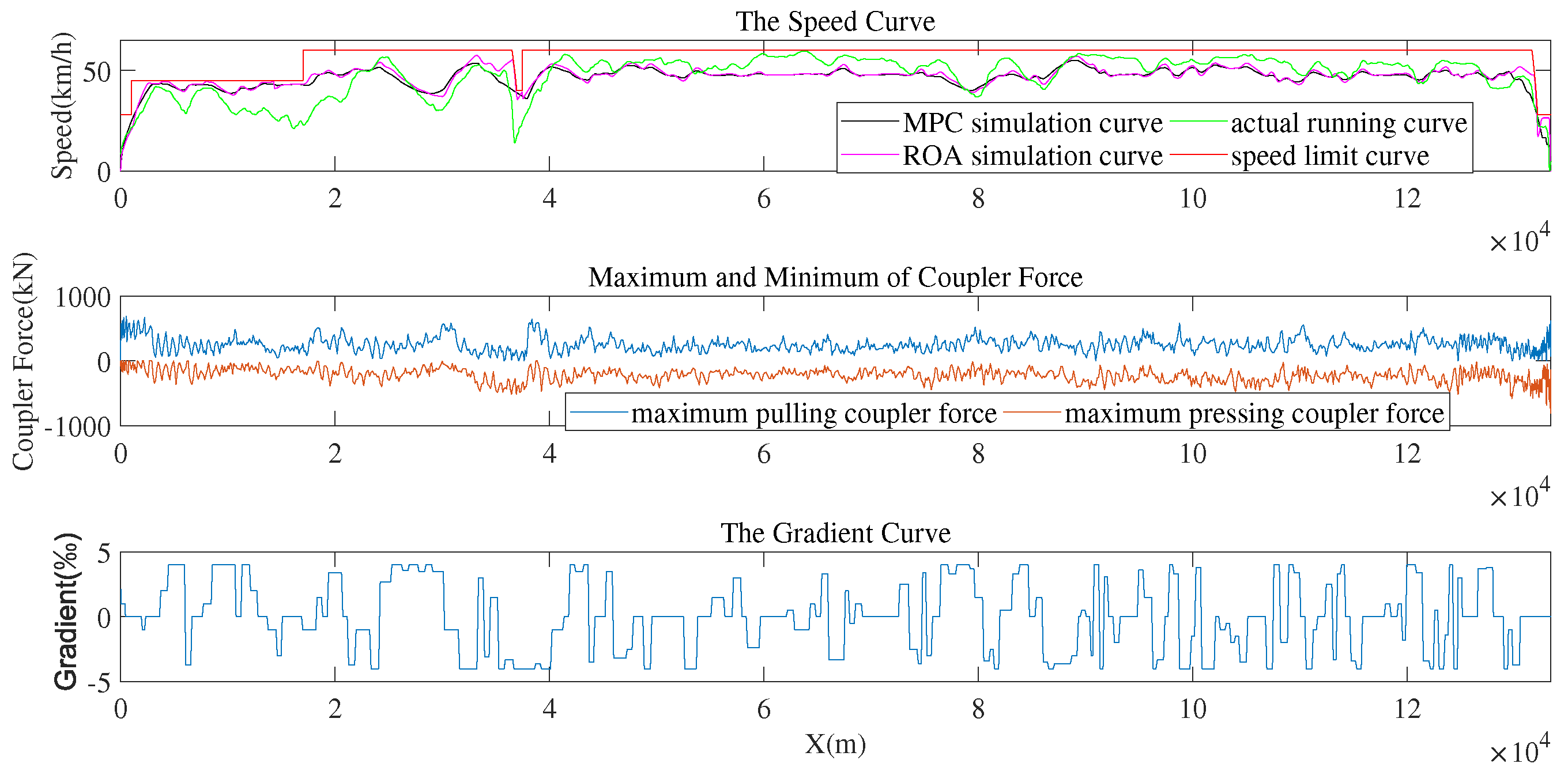
Figure 19.
Control strategy comparison chart

The train fuel consumption based on ROA simulation is 8.09 kg/104 t·km, the train fuel consumption based on MPC algorithm simulation is 6.71 kg/104 t·km, and the actual train fuel consumption calculated by LKJ data is 8.49 kg/104 t·km. Therefore, the Two-step Optimization Method can reduce energy consumption by 20.9% and 17.1% compared to actual operation and ROA simulation respectively.
4. Discussion
In this paper, a Two-step Optimization Method of freight train speed curve is proposed. The Rolling Optimization Algorithm is used to optimize the speed curve, and the optimized speed curve is used as the reference curve of MPC algorithm for the second optimization step. The ROA takes into account the gradient equivalence method and the single-mass train model, while the MPC algorithm employs a multi-mass train model to consider in-train forces and establish an objective function. The optimal train operation results formed by different parameters are calculated by adjusting the weight coefficients of the objective function and the prediction step and optimization step of the MPC algorithm.
Our simulation results, based on data from China’s Dalailong railway, demonstrate that the speed curves generated by the Two-step Optimization Method exhibit superior smoothness and are more aligned with actual operational constraints. Compared to actual operations, this method achieves a remarkable 20.9% reduction in energy consumption, and a 17.1% reduction when compared to the ROA simulation. The optimized throttle sequences require less frequent adjustments, providing a more practical guide for drivers during actual operations.
Looking ahead, we plan to further test and refine the train suggested speed curve optimization program based on the outcomes of the Two-step Optimization Method. The ultimate goal is to integrate this optimization algorithm into the Driver Advisory System (DAS) to offer drivers a more effective reference, thereby reducing train energy consumption and enhancing the overall efficiency of freight train operations.
Author Contributions
Conceptualization, X.S.; methodology, J.L. and W.Z.; formal analysis, J.L.; investigation and data curation, G.S. and X.Z.; writing—original draft, J.L.; writing—review and editing, W.Z.; supervision, X.S.; funding acquisition, H.X. All authors have read and agreed to the published version of the manuscript.
Funding
This work was supported by the National Key R&D Program of China (2023YFB4302104-1)
Data Availability Statement
The data are available upon request.
Acknowledgments
This work was supported by the National Key R&D Program of China
Conflicts of Interest
The authors declare no conflicts of interest. The funders had no role in the design of the study; in the collection, analyses, or interpretation of data; in the writing of the manuscript; or in the decision to publish the results.
Abbreviations
The following abbreviations are used in this manuscript:
| DAS | Driver Advisory System |
| ROA | Rolling Optimization Algorithm |
| MPC | Model Predictive Control |
| ATO | Automatic Train Operation |
| LQR | Linear Quadratic Regulator |
| NSGA-II | Non-dominated Sorting Genetic Algorithm-II |
| FAGA | Fuzzy Adaptive Genetic Algorithm |
| PID | Proportion Integration Differentiation |
| LKJ | Train Operation Monitoring Equipment |
References
- National Railway Administration of the People’s Republic of China. Railway Statistics Bulletin 2023. Beijing, China, 2024. [Google Scholar]
- Howlett, P.; Milroy, I.; Pudney, P. Energy-efficient train control. IFAC Proceedings Volumes 1993, 26, 1081–1088. [Google Scholar] [CrossRef]
- Howlett, P.; Pudney, P.; Vu, X. Local energy minimization in optimal train control. Automatica 2009, 45, 2692–2698. [Google Scholar] [CrossRef]
- Pudovikov, O.E.; Bespał’Ko, S.V.; Kiselev, M.D.; Serdobintsev, E.V. Application of a reference train model in an automatic control system of freight-train speed. Russ. Electr. Engin. 2017, 88, 563–567. [Google Scholar] [CrossRef]
- Gruber, P.; Bayoumi, M.M. Suboptimal control strategies for multilocomotive powered trains. In Proceedings of the 19th IEEE Conference on Decision and Control including the Symposium on Adaptive Processes, Albuquerque, NM, USA; 1980; pp. 319–327. [Google Scholar] [CrossRef]
- Chou, M.; Xia, X.; Kayser, C. Modelling and model validation of heavy-haul trains equipped with electronically controlled pneumatic brake systems. Control Engineering Practice 2007, 15, 501–509. [Google Scholar] [CrossRef]
- Zhuan, X.; Xia, X. Speed regulation with measured output feedback in the control of heavy haul trains. Autom 2008, 44, 242–247. [Google Scholar] [CrossRef]
- Howlett, P.G.; Cheng, J. Optimal driving strategies for a train on a line with continuously varying gradient. The Journal of the Australian Mathematical Society. Series B. Applied Mathematics 1997, 38, 388–410. [Google Scholar] [CrossRef]
- Khmelnitsky, E. On an optimal control problem of train operation. IEEE Transactions on Automatic Control 2000, 45, 1257–1266. [Google Scholar] [CrossRef]
- Martinis, V.D.; Weidmann, U.A. Improving energy efficiency for freight trains during operation: The use of simulation. In Proceedings of the 2016 IEEE 16th International Conference on Environment and Electrical Engineering (EEEIC); Florence, Italy, 2016; pp. 1–6. [Google Scholar] [CrossRef]
- Ko, H.; Koseki, T.; Miyatake, M. Application of dynamic programming to optimization of running profile of a train. Computers in Railways IX 2004, 103–112. [Google Scholar]
- Albrecht, T.; WGassel, C.; Binder, A.; van Luipen, J. Dealing with operational constraints in energy efficient driving. In Proceedings of the IET Conference on Railway Traction Systems (RTS 2010), Birmingham; 2010; pp. 1–7. [Google Scholar] [CrossRef]
- Guo, Y.; Qiu, L.; Ma, J.E. Multi-objective optimization of high-speed train running speed trajectory based on particle swarm and NSGA-II fusion algorithm. In Proceedings of the 2022 IEEE Transportation Electrification Conference and Expo, Asia-Pacific (ITEC Asia-Pacific); Haining, China, 2022; pp. 1–5. [Google Scholar] [CrossRef]
- Yi, L.Z.; hang, D.K.; Li, W. Research on multi-objective optimization of freight train operation process based on improved bald eagle search algorithm. Journal of Computers 2022, 33, 135–150. [Google Scholar]
- Yang, H.; Xu, K.X.; Fu, Y.T. Research on multi-objective optimal control of heavy haul train based on iImproved genetic algorithm. In Proceedings of the 2022 4th International Conference on Industrial Artificial Intelligence (IAI); Shenyang, China, 2022; pp. 1–6. [Google Scholar] [CrossRef]
- Isna, S.S.; Ari, S. Application of model predictive control on metro train scheduling problems. International Journal of Vehicle Information and Communication Systems 2023, 8, 103–118. [Google Scholar] [CrossRef]
- Song, Y.X. Research on train automatic operation control algorithm for heavy-hual trains based on model predictive control. M.S. thesis, Southwest Jiaotong Univ., Chengdu, Sichuan, China, 2022. [Google Scholar]
- Liu, Y.; Zhang, Z.F.; Jiang, F. Research on model predictive control method of heavy-haul trains based on multi-point model. In Proceedings of the 2023 IEEE Vehicle Power and Propulsion Conference (VPPC); Milan, Italy, 2023; pp. 1–7. [Google Scholar] [CrossRef]
- He, X.M.; Wang, S.; Alanamu, B.B. Research on optimal train adhesion control based on nonlinear model predictive control. In Proceedings of the International Conference on Smart Transportation and City Engineering (STCE 2023), Chongqing, China; 2023. [Google Scholar] [CrossRef]
- Zhang, L.J.; Li, Q.; Zhuan, X.T. Energy-efficient operation of heavy haul trains in an MPC framework. In Proceedings of the 2013 IEEE International Conference on Intelligent Rail Transportation Proceedings, Beijing, China; 2013; pp. 105–110. [Google Scholar] [CrossRef]
- Zhang, L.J.; Zhuan, X.T.; Xia, X.H. Optimal operation of heavy haul trains using model predictive control methodology. In Proceedings of the 2011 IEEE International Conference on Service Operations, Logistics and Informatics, Beijing, China; 2011; pp. 402–407. [Google Scholar] [CrossRef]
- Zhang, L.J.; Zhuan, X.T. Optimal operation of heavy-haul trains equipped with electronically controlled pneumatic brake systems using model predictive control methodology. IEEE Transactions on Control Systems Technology 2014, 22, 13–22. [Google Scholar] [CrossRef]
- Zhang, L.J.; Zhuan, X.T. Development of an Optimal Operation Approach in the MPC Framework for Heavy-Haul Trains. IEEE Transactions on Intelligent Transportation Systems 2015, 16, 1391–1400. [Google Scholar] [CrossRef]
- Zhang, W. Research on receding optimization of energy-saving speed curve of freight trains. M.S. thesis, Beijng Jiaotong Univ., Beijing, China, 2023. [Google Scholar]
- Bujarbaruah, M.; Zhang, X.J.; Borrelli, F. Adaptive MPC with Chance Constraints for FIR Systems. In Proceedings of the 2018 Annual American Control Conference (ACC), Milwaukee, WI, USA; 2018; pp. 2312–2317. [Google Scholar] [CrossRef]
- Zhai, W.M. Research on the dynamics performance evaluation standard for freight trains and the suggested schemes(last part continued)—evaluation standard for vertical wheel rail force and coupler force. Rolling Stock 2002, 03, 10–13+1. [Google Scholar]
Figure 1.
Two-step Optimization Method framework
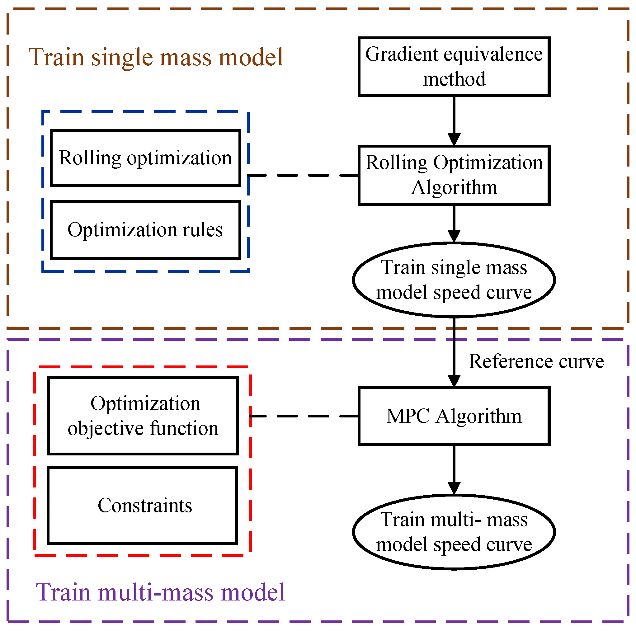
Figure 2.
Comparison of the original and the equivalent gradient
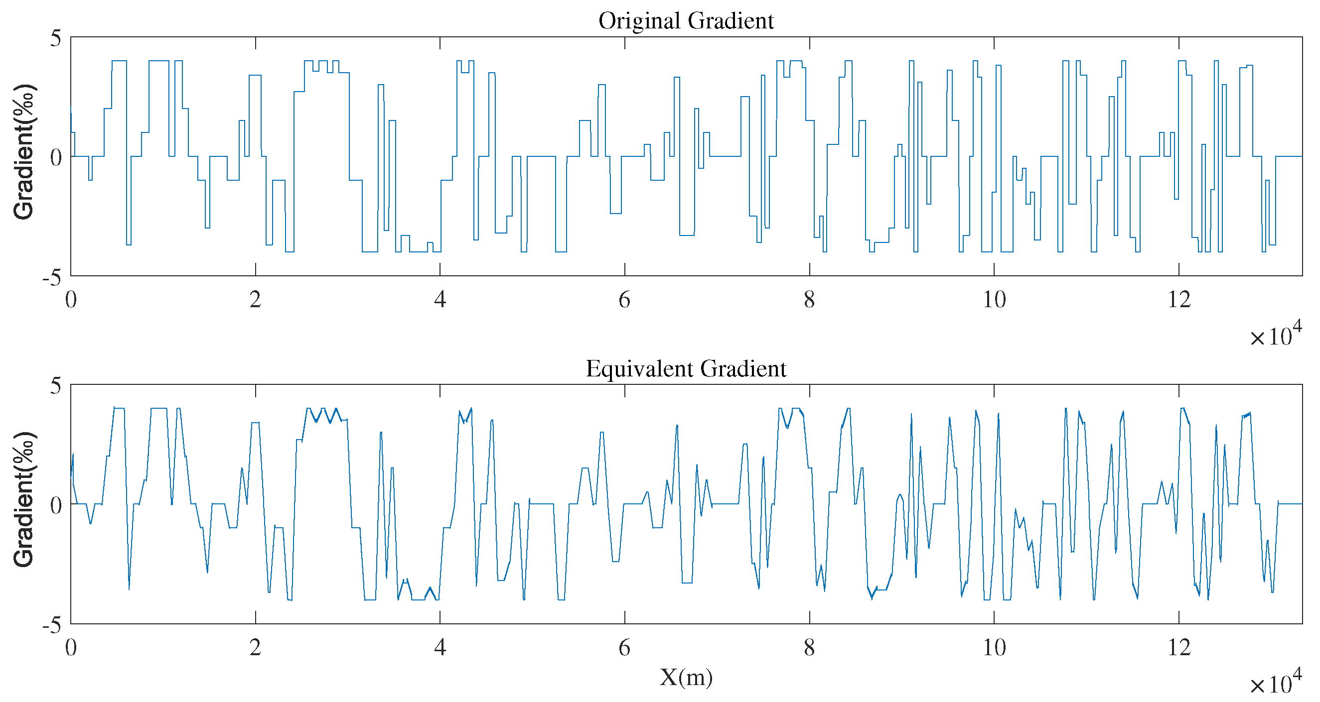
Figure 3.
Slope type demonstration
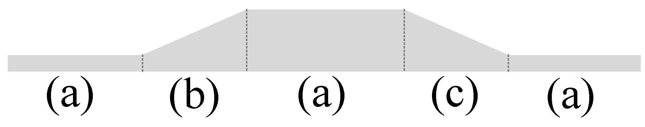
Figure 4.
Flowchart of Rolling Optimization Algorithm for freight train speed curve
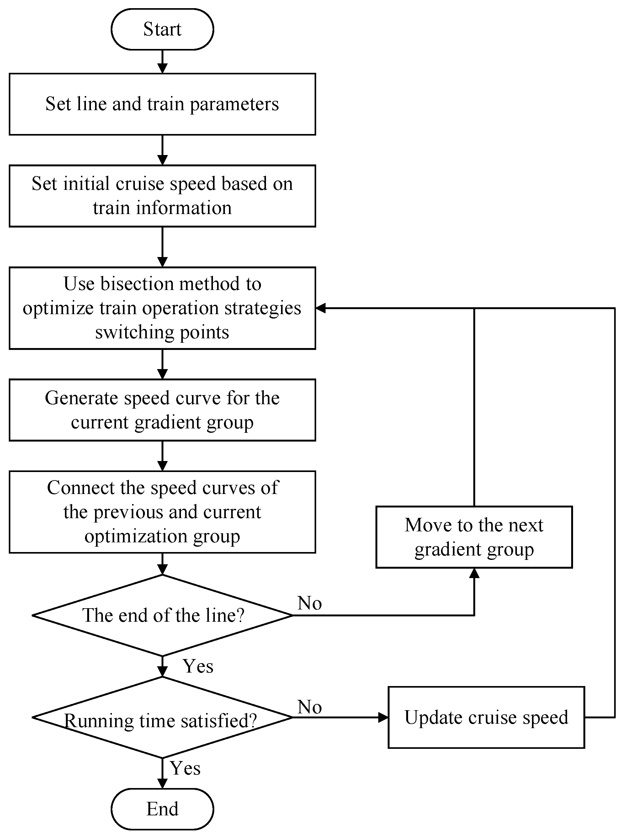
Figure 5.
Comparison of the traction switching points for the uphill section
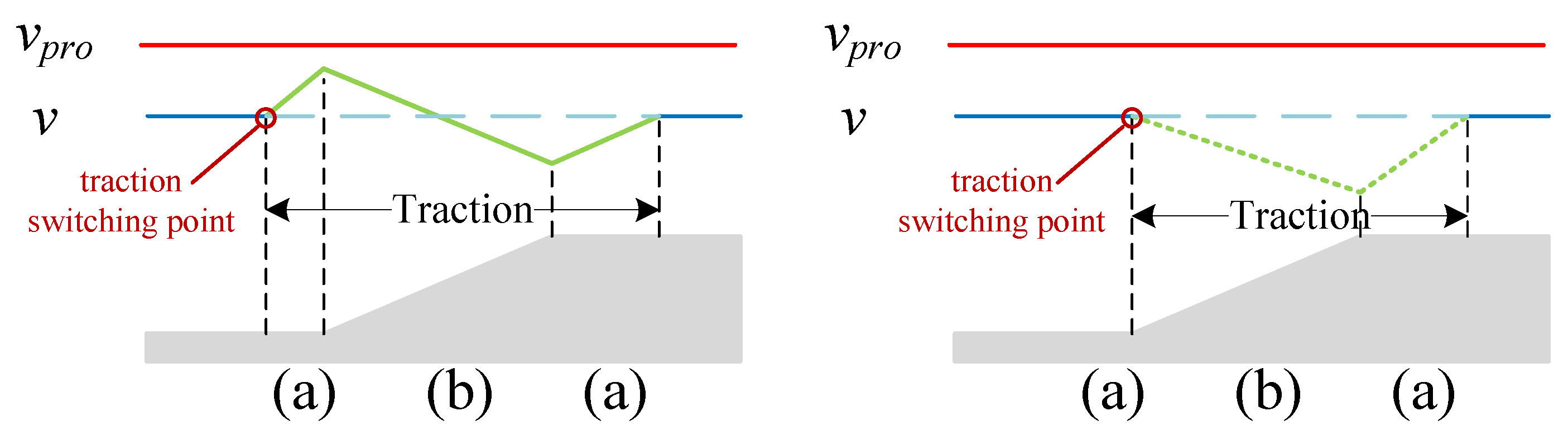
Figure 6.
Comparison of the coast switching points for the downhill section
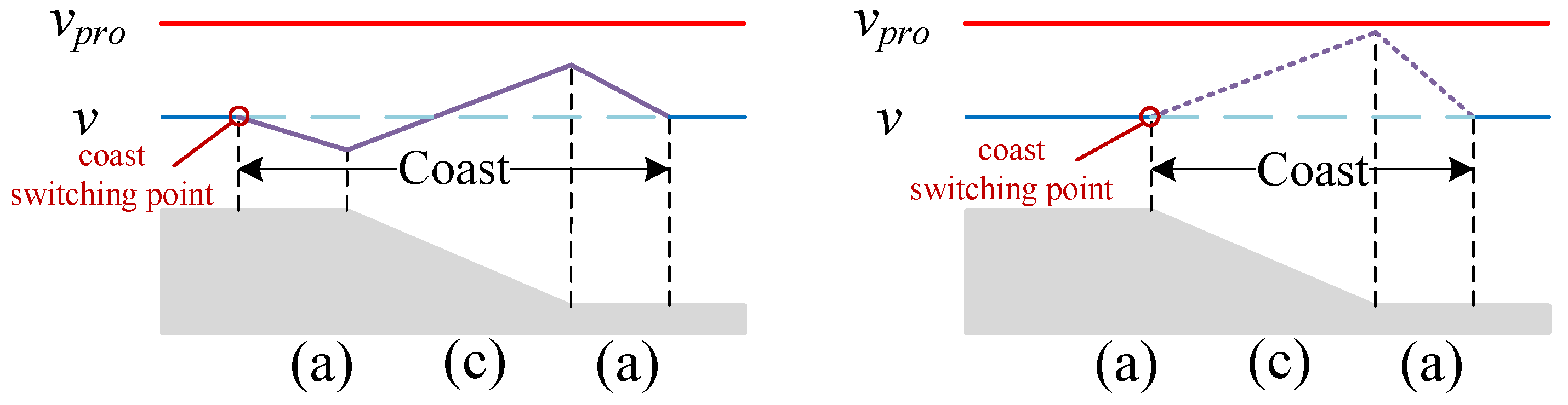
Figure 7.
Speed curves connecting method
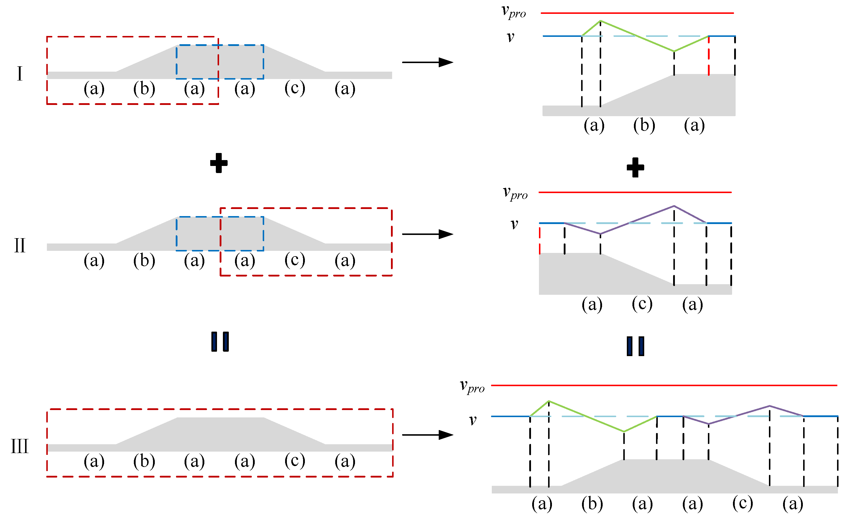
Figure 8.
MPC algorithm demonstration
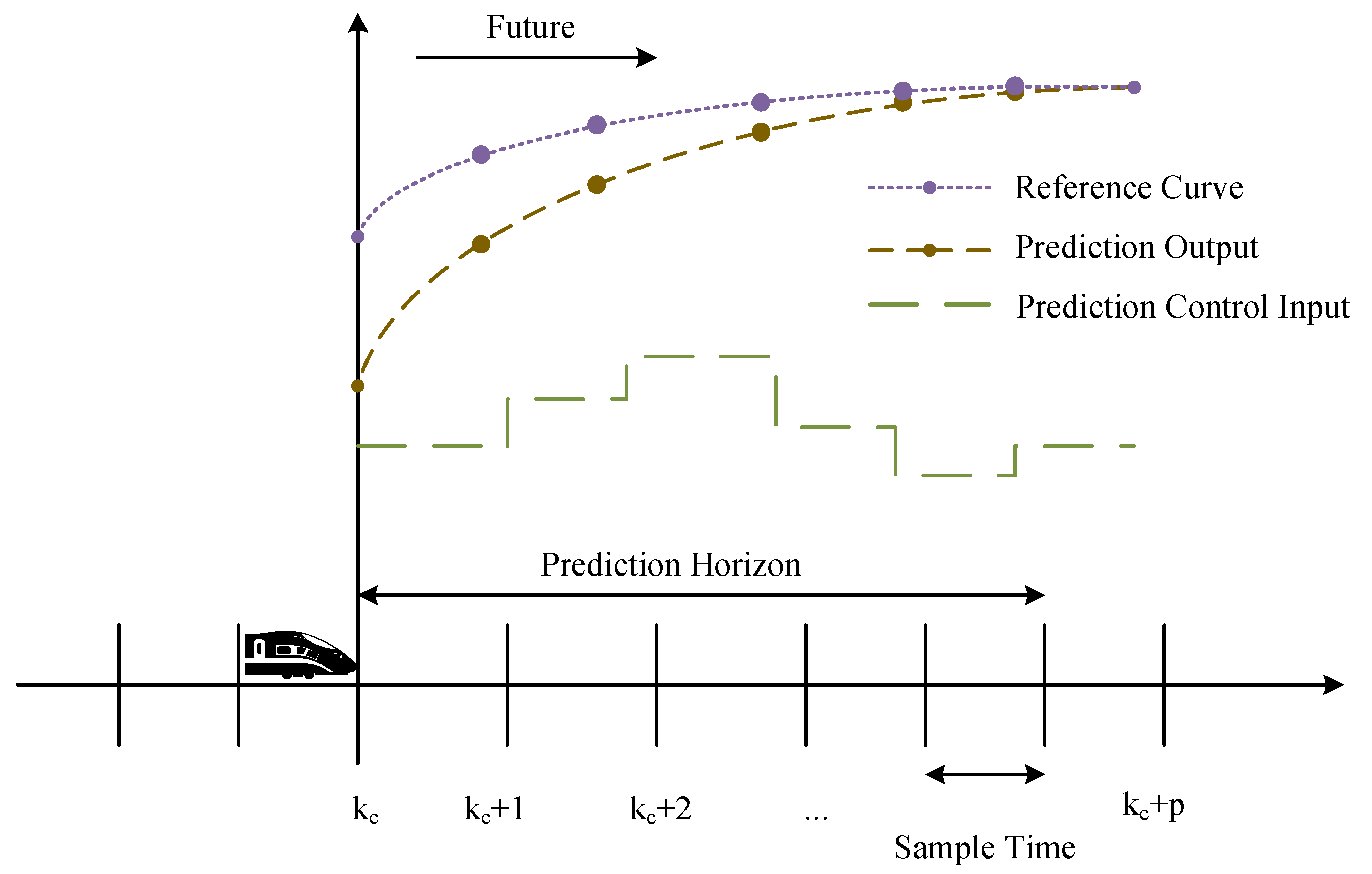
Figure 9.
Train multi-mass model
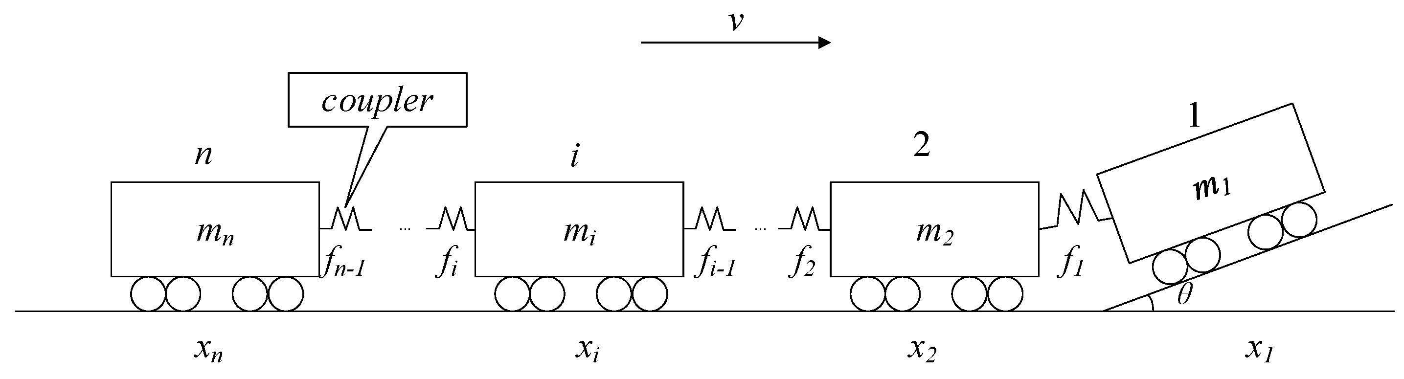
Figure 10.
Force analysis for a single locomotive/wagon
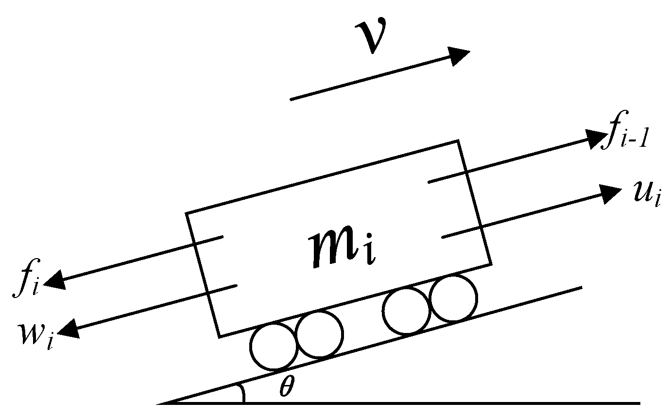
Figure 11.
Coupler force with different when = 0.1, = 10
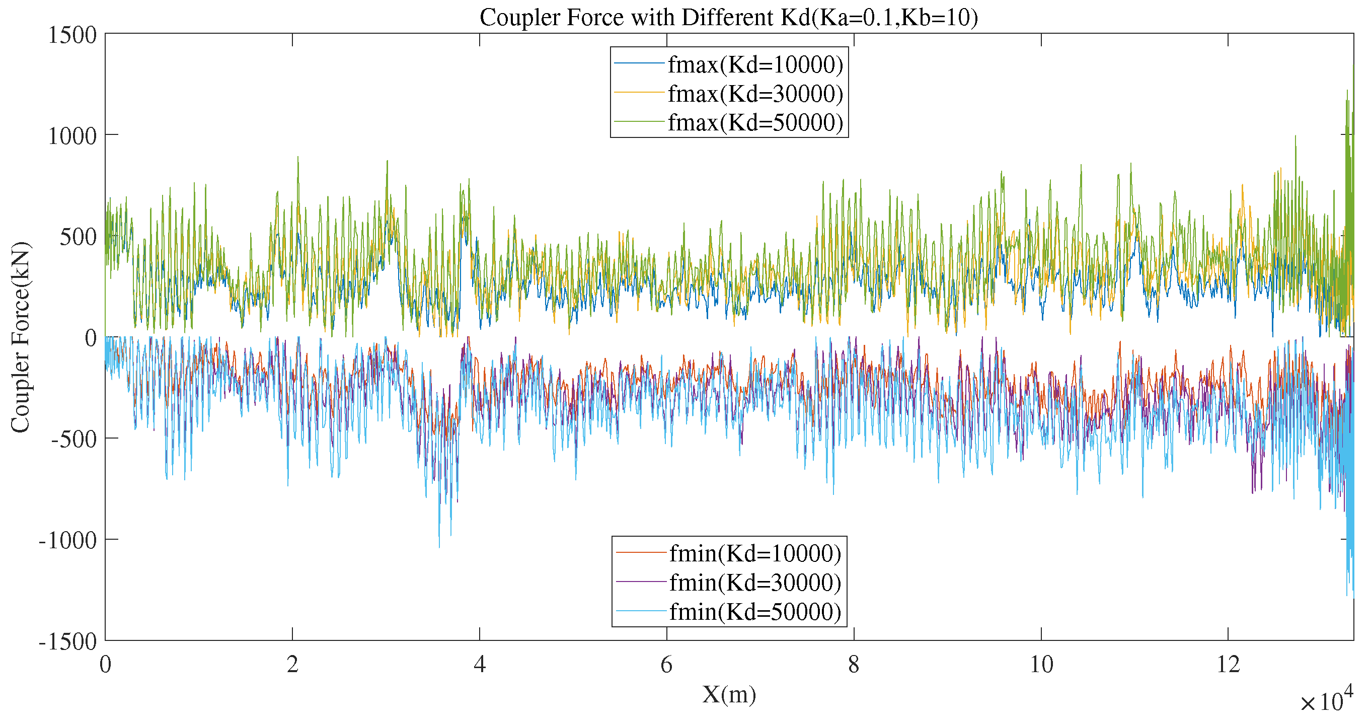
Figure 12.
Coupler force with different when = 0.01, = 10
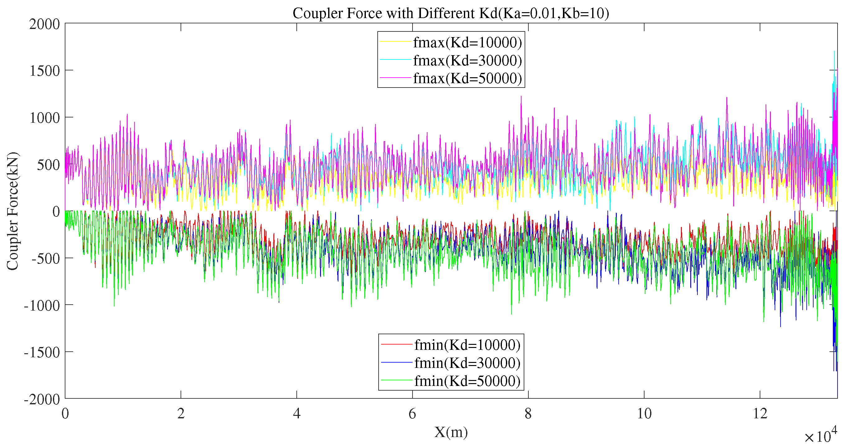
Figure 13.
Simulation speed curves with different weighting coefficients
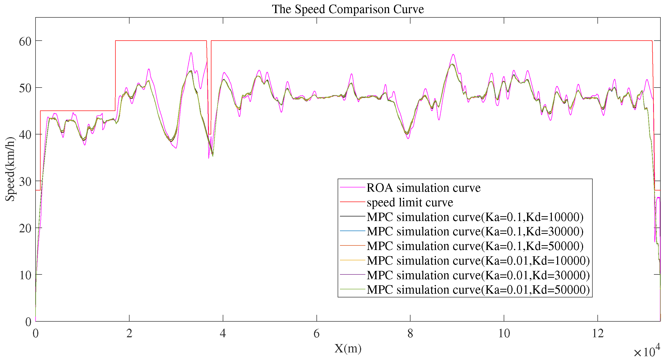
Figure 14.
Partially enlarged simulation speed curves with different weighting coefficients
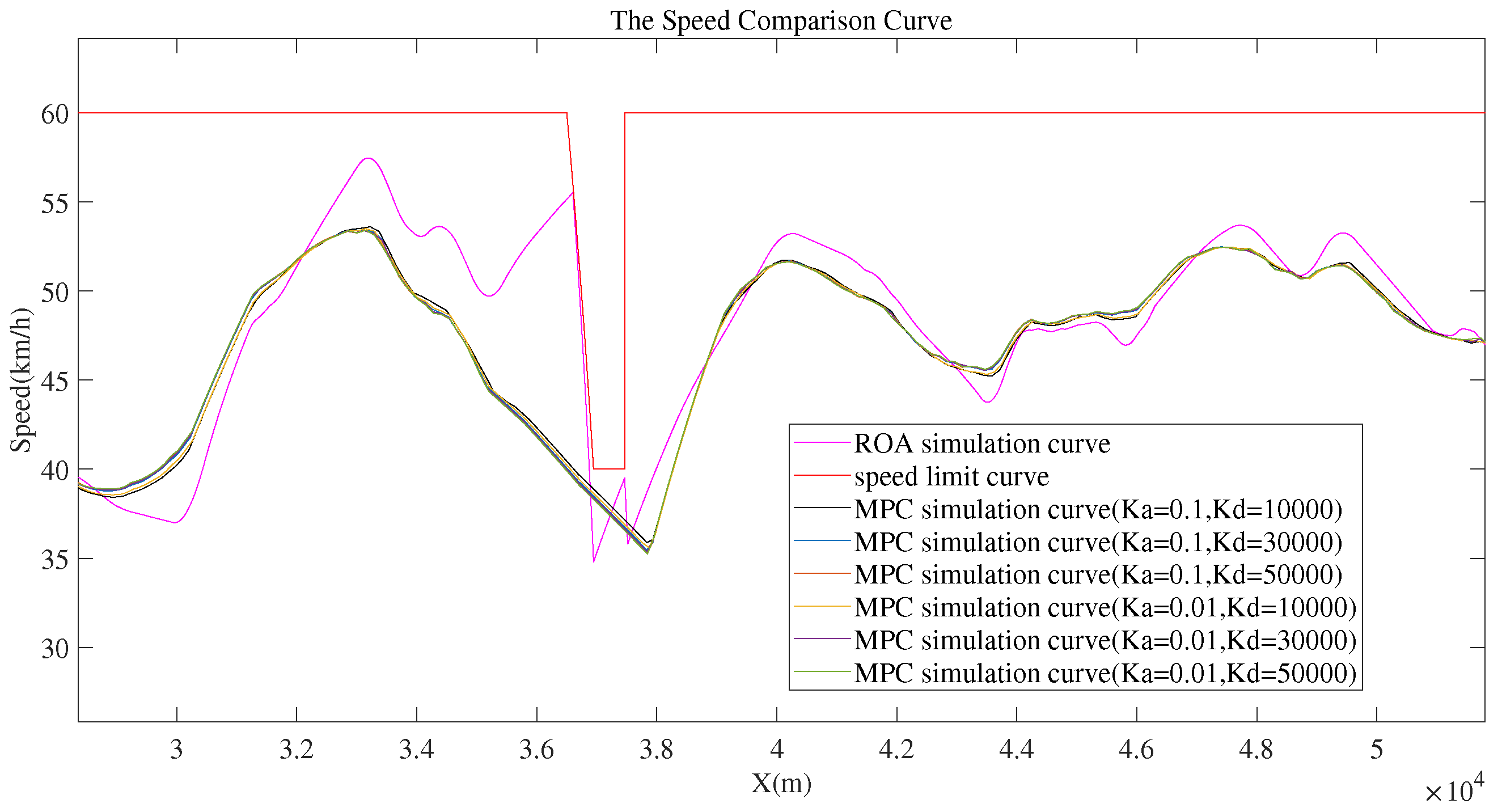
Figure 15.
Coupler force with different and
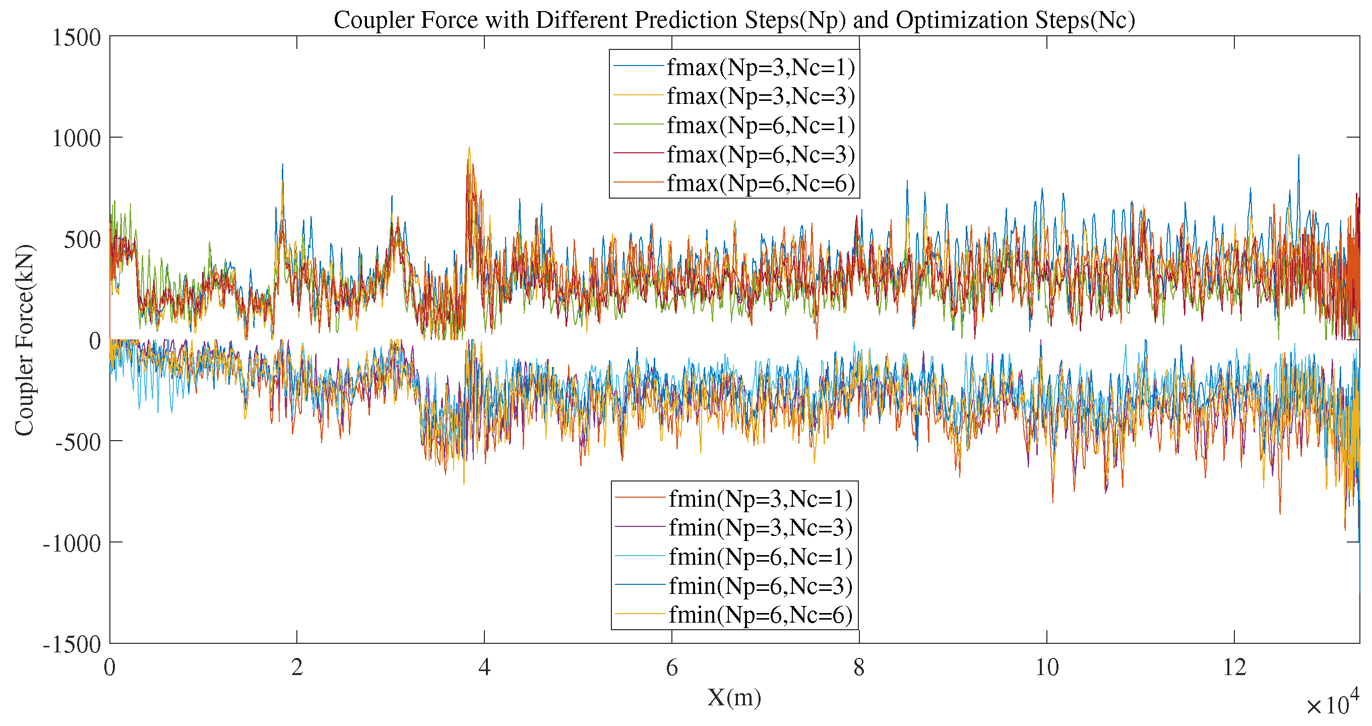

Table 1.
Classification of gradient types
| Gradient Types | Gradient Values | Type Symbols |
|---|---|---|
| General section | a | |
| Steep uphill section | b | |
| Downhill section | c | |
| Steep downhill section | d |
Table 2.
Train operation results with different objective function weights
| 0.1 | 10 | 10000 | 687.2 | -804.2 | 20 |
| 0.1 | 10 | 30000 | 838.9 | -983.5 | 15 |
| 0.1 | 10 | 50000 | 1343.6 | -1292.4 | 25 |
| 0.01 | 10 | 10000 | 1021.8 | -1034.6 | 15 |
| 0.01 | 10 | 30000 | 1701.7 | -1974.5 | 20 |
| 0.01 | 10 | 50000 | 1520.9 | -1604.7 | 25 |
Table 3.
Train operation results with different prediction steps and optimization steps
| 6 | 6 | 763.9 | -875.8 | 35 |
| 6 | 3 | 831.9 | -1005.4 | 35 |
| 6 | 1 | 687.2 | -804.2 | 20 |
| 3 | 3 | 785.7 | -706.5 | 160 |
| 3 | 1 | 868.4 | -851.1 | 150 |
Disclaimer/Publisher’s Note: The statements, opinions and data contained in all publications are solely those of the individual author(s) and contributor(s) and not of MDPI and/or the editor(s). MDPI and/or the editor(s) disclaim responsibility for any injury to people or property resulting from any ideas, methods, instructions or products referred to in the content. |
© 2025 by the authors. Licensee MDPI, Basel, Switzerland. This article is an open access article distributed under the terms and conditions of the Creative Commons Attribution (CC BY) license (http://creativecommons.org/licenses/by/4.0/).
Copyright: This open access article is published under a Creative Commons CC BY 4.0 license, which permit the free download, distribution, and reuse, provided that the author and preprint are cited in any reuse.


