
Submitted:
23 December 2024
Posted:
25 December 2024
Read the latest preprint version here
Abstract
In model calibration, the identification of the unknown parameter values itself but also the uncertainty of these model parameters due to uncertain measurements or model outputs might be required. The analysis of the parameter uncertainty helps to understand the calibration problem better. Investigations on the parameter sensitivity and the uniqueness of the identified parameters could be addressed within the uncertainty quantification. In this paper we investigate different probabilistic approaches for this purpose, which identify the unknown parameters as multivariate distribution function. However, these approaches require the accurate knowledge of the model output covariance which is often not available. Alternatively, we investigate interval optimization methods for the identification of parameter bounds. The correlation or interaction of the input parameters can be modeled by a convex feasible domain which belongs to feasible solution of the model output within given bounds. We will introduce a radial line-search procedure which can identify the boundary of such a parameter domain for arbitrary non-linear dependencies between model input and output.
Keywords:
model calibration
; parameter identification
; uncertainty quantification
; inverse problems
; Bayesian updating
; interval optimization
1. Introduction
Within the calibration of material models, the numerical results of a simulation model are compared with the experimental measurements as illustrated in Figure 1.
One common approach is to minimize the squared errors between the simulation response and the measurements, the so-called least squares approach [1]
This minimization task can be solved by a single-objective optimization algorithm to obtain the optimal parameter set . The optimization procedure requires special attention, if the optimization task is not convex and contains several local minima as discussed in [2,3,4]. A recent overview of optimization techniques to solve the calibration task is given in [5,6]. Often a maximum likelihood approach [1] is used to formulate the optimization goal. To ensure a successful identification with optimization techniques, the sensitivity of the model parameters with respect to the considered model outputs should be investigated initially as discussed in [7].
Additionally to the parameter values itself, the estimation of the parameter uncertainty due to scatter in the experimental measurements and inherent randomness of the material properties requires further investigations. In [1,8] a straight-forward linearization based on the maximum likelihood approach was introduced, where the parameter scatter is assumed as a multi-variate normal distribution. A generalization of this method is the Bayesian updating technique [1], where the joint distribution function of the model parameters can be obtained only implicitly from the model input-output dependencies in many cases. A good overview and recent developments of this technique are given e.g. in [9,10,11,12,13]. Since the parameter distribution function can be obtained in closed form only for special cases, inverse sampling procedures such as Markov Chain Monte Carlo methods (MCMC) are usually applied to generate discrete samples of the unknown multi-dimensional parameter distribution [14]. Most of these methods rely on the original Metropolis-Hastings algorithm [15]. However, the MCMC methods require usually a large number of model evaluations and meta-models are often applied to accelerate the identification procedure [2,16]. Additionally, the Bayesian updating approach requires an accurate estimate of the measurement covariance matrix which is often not available. In the following paper we want to investigate this problem in detail.
Additionally to probabilistic methods, interval approaches have been developed which model the uncertainty of the model inputs and outputs as interval numbers [17,18] or confidence sets [19]. Based on this assumption, interval predictor models have been used for model parameter identification [20]. The unknown model parameter bounds can be obtained for inverse problems from the given model output bounds by interval optimization methods [21,22]. In [23] interval optimization was introduced for fuzzy numbers to obtain a quasi-density of unknown model outputs in forward problems. However, this method can also be applied to inverse problems which results usually in minimum and maximum values for each parameter considered in the model calibration. In [24,25] bounding boxes have been used to represent the multi-dimensional domain of the feasible input parameter space. This idea has been extended quite recently to consider correlations between the model parameters [26,27].
Let us introduce the following uniaxial bilinear elasto-plasticity model as an illustrative example
where is the uniaxial stress depending on the uniaxial strain . The model parameters are the Young’s modulus E, the yield stress and the hardening modulus H. In Figure 2 the reference curve is given for a selected parameter set , and .
If we assume, that the measurement points contain some scatter or uncertainty, the calibrated optimal parameter set could show significant deviation from the reference parameters as shown in Figure 2, where an additional Gaussian noise term is used to generate synthetic measurement points
where is a normally distributed random number with zero mean and unit variance. If we repeat the calibration of the model with different samples of the noise term, the calibrated optimal parameters will show a certain scatter which depends on the size of the noise term. 1000 samples of the calibrated parameters are shown exemplarily in Figure 3 for a of noise term of by considering 20 measurement points as shown in Figure 2. The figure indicates, that all three identified parameter show significant scatter and the yield stress and the hardening modulus show a significant correlation to each other.
In the following paper, we will investigate different methods to estimate the uncertainty of the calibrated parameters from given measurement uncertainty. Based on classical probabilistic approaches as the maximum likelihood estimator or the Bayesian updating procedure, the scatter of the identified parameters can be estimated as a multi-variate probability density function. Both procedures require a sufficient accurate knowledge or estimate of the scatter of the measurement points, often modeled by a Gaussian covariance matrix. Furthermore, we present an additional approach by assuming the scatter of the measurements not as correlated random numbers but as individual intervals with known minimum and maximum values. The corresponding possible minimum and maximum values for each input parameter can be obtained for this assumption using a constrained optimization procedure. However, the identification of the whole possible parameter domain for the given measurement bounds is not straight forward. Therefore, we introduce an efficient line-search method, where not only the bounds itself but also the shape of the feasible parameter domain can be identified. This enables the quantification of the interaction and the uniqueness of the input parameters. Furthermore, we put emphasis on the initial sensitivity analysis, which should be considered for all approaches to neglect unimportant parameters in the calibration procedure. As a numerical example, we identify the fracture parameters of plain concrete with respect to a wedge splitting test, where six unknown material parameters should be identified.
2. Sensitivity Analysis of the Model Parameters
In order to obtain a sufficient accuracy of the calibrated model parameters a certain sensitivity of these parameters with respect to the model responses is necessary. If all model responses are not sensitive with respect to a specific parameter, this parameter can not be identified within an inverse approach. In such a case, this parameter should be kept fixed and not considered in the calibration process.
A quite common approach for a sensitivity analysis is a global variance-based method using Sobol indicices [28,29]. In this method the contribution of the variation of the input parameters with respect to the variation of a certain model output can be analyzed. Originally, this method was introduced for sensitivity analysis in the context of uncertainty quantification, but it can similarly applied for optimization problems as discussed in [30].
If we define lower and upper bounds for the m unknown model parameters
we can assume a uniform distribution for each parameter
The variance contribution of the parameter with respect to a model output can be quantified with the first order sensitivity measure introduced by [28]
where is the unconditional variance of and is called the variance of conditional expectation with denoting the set of all parameters but . measures the first order effect of on the model output. Since first order sensitivity indices quantify only the decoupled influence of each parameter, the total effect sensitivity indices have been introduced by [29] as follows
where measures the first order effect of on the model output which does not contain any effect corresponding to .
Generally, the computation of and requires special estimators with a large number of model evaluations [31]. In [32,33] regression based estimators have been introduced, which require only a single sample set of the model input parameters and the corresponding model outputs. One very simply estimator for the first order index is the squared Pearson correlation coefficient
The Pearson correlation assumes a linear dependence between model input and output. If this is fulfilled, the sum of the first order indices should be close to one. However, if the model output is a strongly nonlinear function of the parameters, the sum is smaller than one and a reliable estimate is not possible with this approach.
With the Metamodel of Optimal Prognosis (MOP) [33] a more accurate meta-model based approach for variance-based sensitivity analysis was introduced, where the quality of the meta-model is estimated with the Coefficient of Prognosis (CoP) by means of a sample cross-validation. If the CoP is close to one, the meta-model can represent the main part of the model output variation and thus the sensitivity estimates are sufficiently accurate. In the MOP approach different types of meta-models such as classical polynomial response surface models [34,35], Kriging [36], Moving Least Squares [37] as well as artificial neural networks [38] are tested automatically for a specific model output and evaluated by means of the CoP measure. This approach is available with the Ansys optiSLang software package [39]. Further information on the overall framework and the CoP measure can be found in [40,41]. The samples for the regression based estimators can be generated pure randomly within the defined parameter bounds. However, in order to increase the accuracy of the sensitivity estimates, we apply an improved Latin Hypercube sampling (LHS) [42], which reduces the spurious correlations between the inputs parameters.
In Figure 4 the sensitivity indices from the squared Pearson correlations are shown for the bilinear example by evaluating 20 points on the stress-strain curve. 1000 Latin Hypercube samples have been generated by considering the following parameter bounds: , and .
The figure clearly indicates, that the Young’s modulus shows a significant influence for smaller strain values whereas the yield stress and the hardening modulus become more important with increasing strains. However, the sum of the individual sensitivity indeces is not close to one for strain values between 0.2 and 0.6 % which is caused be the non-linear relation between these stress values with respect to the model parameters. The results of the sensitivity analysis by using the MOP approach are given additionally in the figure and show a similar behavior as the correlation based estimates. However, the approximation quality of the underlying meta-model is almost excellent for all stress values. Thus, the estimated total effect indeces are more reliable measures to judge on the sensitivity of the model parameters for this example.
3. Probabilistic Approaches
3.1. Maximum Likelihood Approach
In the maximum likelihood approach [1,8] the likelihood of the parameters is defined to be proportional to the conditional probability of the measurements for a given parameter set
By assuming that the chosen model can represent the material behavior perfectly, the remaining gap between model responses and experimental observations can be explained only by measurement errors. In this case, is equivalent to the probability of reproducing the measurement errors. Assuming a multivariate normal distribution for the measurement errors yields [8]
where is the covariance matrix of the measurement uncertainty. Maximizing the likelihood L is equivalent to minimize and yields to the following objective function
If the measurement errors are assumed to independent, the objective function equals a weighted least squares formulation
where the weight factor for each measurement value is the inverse of its variance . For constant measurement errors this objective simplifies to the well-known least squares formulation introduced in Eq. 1. In this case the optimal parameter set with the maximum likelihood approach can be obtained by standard optimization procedures without exact knowledge of the measurement covariance matrix.
3.2. Markov estimator
The objective function in Eq. 11 can be linearized as follows [8]
where is a sensitivity matrix, which contains the partial derivatives of the model responses with respect to the parameters
Assuming, that the optimal parameter set has been found by minimizing the objective function, we can estimate the sensitivity matrix at the optimal parameter set e.g. by a central differences method.
Assuming a linear relation between the model parameters and responses, the covariance matrix of the parameters can be estimated with the so-called Markov estimator [1,8]
This covariance matrix contains the necessary information about the scatter of the individual parameters as well as possible pairwise correlations. The distribution of the parameters is Gaussian as assumed for the measurements. The estimated scatter and correlations are a very useful information to judge about the accuracy and uniqueness of the identified parameters in a calibration process. This method can be interpreted as an inverse first order second moment method: assuming a linear relation between parameters and measurements and a joint normal distribution of the measurements, we can directly estimate the joint normal covariance of the parameters. However, the application of this linearization scheme requires an accurate estimate of the optimal parameter set by a previous least squares minimization. Furthermore, the inversion of the matrix in Eq. 15 requires, that every parameter is sensitive w.r.t. the model output. This should be investigated with an initial sensitivity analysis as explained in Section 2.
The evaluation of Eq. 15 requires an estimate of the measurement covariance matrix . If a measurement procedure is repeated very often, this matrix can be estimated directly from measurement statistics. However, this is often not possible. A valid estimate could be to assume independent measurement errors. The resulting covariance matrix is then diagonal, where at least the scatter of the individual measurement points has to be estimated. From a small number of measurement repetitions this can be estimated straight forward. If even such information is not available, the measurement scatter can be assumed to be constant for each output value
In this case, the estimated covariances of the parameters are directly scaled by the assumed measurement scatter
If only a single measurement curve is available for the investigated responses, the misfit of the calibration process can be used for a rough estimate. Assuming the measurement errors to be constant and independent, we obtained the following estimate
where n is the number of measurement points.
In Figure 5 the estimated scatter of the parameters of the bilinear model is shown. Again 20 measurement points with are assumed, which results in a covariance matrix according to Eq. 16. The figure indicates a similar scatter and correlation of the parameters as obtained with the 1000 calibration runs in Figure 3. For the calculation of the sensitivity matrix in Eq. 14 only 6 model evaluations are necessary.
The sensitivity matrix in Eq. 14 can be visualized as shown in Figure 6 by normalizing the partial derivatives with respect to the parameter ranges
By using the variance formula for a sum of linear factors, we can estimate local variance-based first order sensitivity indices from this partial derivatives by assuming again a uniform distribution of the parameters within the defined bounds
In Figure 7 the estimated parameter scatter normalized with the parameter ranges is shown depending on the size of an independent measurement error according to Eq. 16 for 20 measurement points. The figure indicates a linear relation of the standard deviation of all parameters as expected from the formulation in Eq. 17. The normalized parameter scatter of the yield stress is significantly smaller compared to the scatter of the Young’s and hardening moduli. This is caused by the fact, that sensitivity of the yield stress is on average larger as observed in the normalized partial derivatives in Figure 6. Additionally to the influence of the measurement error, the influence of the number of measurement points is shown in Figure 7 for a constant . The figure clearly indicates, that with an increasing number of independent measurement points, the estimated scatter and thus the uncertainty decreases. This problem is discussed in [43] and could be resolved only, if a realistic correlation between the measurement points is assumed in the covariance matrix.
3.3. Bayesian Updating
Another probabilistic method is the Bayesian updating approach [1], which can represent non-linear relations between the parameters and the responses but requires much more numerical effort to obtain the statistical estimates. In this approach the unknown conditional distribution of the parameters is formulated with respect to the given measurements by using the Bayes’ theorem as follows
The likelihood function can be formulated as probability density function, whereby often a multi-normal distribution function is utilized similarly as by Markov estimator
The so-called prior distribution can be assumed either from previous information or as an uniform distribution within initially defined parameter bounds. Since the normalization term is usually not known, the posterior parameter distribution could not be obtained in closed form. However, in such a case Markov Chain Monte Carlo methods could be used to generate discrete samples of the posterior distribution. A recent overview of these methods is given in [14]. For further details on Bayesian updating the interested reader is referred to [9]. In our study the well-known Metropolis-Hastings algorithm [15] is applied, which considers only the forward evaluation of the likelihood function to generate samples of the posterior distribution. Further details on this algorithm can be found in [2].
In Figure 8 the estimated parameter scatter of the bilinear model is shown by assuming again independent measurement errors of . 20.000 samples have been generated by the Metropolis-Hastings algorithm by neglecting the first 2.000 samples, the so-called burn-in phase. The pair-wise anthill plots and the correlation matrix indicate a good agreement with the results of the Markov estimator in Figure 5 for this example. This can be explained by the approximately linear behavior of the model for small measurement errors.
In Figure 9 the corresponding variation of the response values are given. The figure indicates a good agreement of the mean response values with the deterministic reference curve. Around a deterministic yield strain of a larger deviation could be observed. More interesting is the standard deviation of the individual stress responses. In contrast to the assumption of a constant measurement error of , the variation of all stress values is smaller caused by the inherent correlations of the model responses.
4. Interval Approaches
4.1. Interval Optimization
Instead of modeling the measurement points as correlated random numbers, which requires the estimate of the full covariance matrix, we can assume, that each measurement point is an interval number with known minimum and maximum bounds as shown in Figure 10. For such a given interval of each measurement point, we want to obtain the corresponding range of the model parameters which fulfill
In the classical interval optimization approach, usually the interval of an uncertain response is obtained from the known interval of the input parameters by several forward optimization runs. A specific approach for this purpose, the -level optimization [23], is shown in principle in Figure 10, where the most probable value is assumed for each input parameter with the maximum -level and a linear descent to zero is defined between the maximum and the lower and upper bounds. The -level optimization will detect the shape of the corresponding -levels of the unknown outputs. In an inverse approach, we need to search for the possible minimum and maximum values of the input parameters for a given level, while each response value is constrained to the corresponding interval as defined in Eq. 23. The corresponding constraint optimization task can be formulated for each input parameter as an individual minimization and maximization task as follows
where the specific -level defines the lower and upper bounds and of each response value.
In Figure 11 the obtained minimum and maximum parameter values are shown exemplarily for the bilinear model by considering a constant measurement interval size of . Every optimization run was carried out by using an evolutionary algorithm from the Ansys optiSLang software package [39] with 25 generations and a population size of 20. The obtained best parameter sets of each optimization run are shown in the figure, which span a three-dimensional box around the reference parameter set. However, the figure illustrates that the detection of the lower and upper parameter values alone is not sufficient to investigate the interactions between the input parameters. Therefore, we present a new radial line-search approach in the next section, which investigates the whole multi-dimensional domain of the defined input parameters.
4.2. Radial Line-Search Approach
Assuming interval constrains for each response value according to Eq. 23, the corresponding domain of the feasible input parameter domain is defined as
This domain of feasible parameter sets could be analyzed in case of two input parameters with a line-search approach as illustrated in Figure 12: starting from the optimal parameter set , we search in every direction for the maximum radius of the feasible parameter domain
where is a direction vector of unit length
The direction vectors can be chosen randomly or uniformly distributed as shown in Figure 12 for two input parameters. For each direction a line-search is performed in order to obtained the maximum possible radius for this direction. This search can be realized by bisection or other methods. The obtained boundary points result in a uniform discretization of the feasible parameter domain . This approach is similar to the directional sampling method known from the reliability analysis [44,45].
In Figure 13 the initial radial search points and the obtained boundary points are shown for the 2D subspaces of the three parameter bilinear model by assuming an interval of . The line-search procedure is performed for each subspace separately while keeping the third parameter constant at the reference values. The initial parameter bounds have been chosen from the previous optimization results as , , and and 50 uniformly distributed search directions are considered for each subspace. The subspace plots in Figure 13 indicate an almost rectangular boundary of the feasible Young’modulus-yield stress subspace and of the Young’s modulus - hardening modulus subspace, meanwhile in the third subspace, the yield stress - hardening modulus subspace, the boundary indicates a significant dependence of the feasible parameter values.
In order to extend this method to more than two input parameters, the search directions have to be discretized on a 3D- or higher dimensional (hyper-) sphere. One very efficient discretization method to obtain almost equally distributed points on the hyper-sphere are the Fekete point sets [46], which are generated using a minimum potential energy criterion
where is the number of points on the unit hyper-sphere. The minimization of the potential energy results in equally distributed point sets and will require a significant smaller number of model evaluations to obtain a suitable representation of the parameter domain boundary. An efficient optimization procedure to solve Eq. 28 is proposed in [46]. Once the initial points have been generated, a line-search is performed for each of the search directions similarly as in two dimensions. This search procedure is performed in our study by using a simple bisection method [47]. However, since every direction can be evaluated independently, a parallel computing of the required model evaluations is possible. The obtained points on the boundary can be used to visualize a discretized shape of the feasible parameter domain. If more than two or three parameters are investigated, this visualization could be displayed in 2D or 3D subspaces.
In Figure 14 the initial search points are shown for the bilinear example on the 3D sphere by considering the parameter bounds of the 2D analysis. The figure indicates a very uniform distribution of the points. Additionally, the figure shows the final line-search points for these 500 directions, where each point has been obtained by 10 bisection steps along the specific direction. The figure shows a Delaunay triangulation of the convex hull of these points utilizing the MATLAB plotting library [48]. The obtained feasible parameter domain indicates a dependence between yield stress and hardening modulus similar to the 2D analyses. The ranges of the response values of the obtained boundary points are given in Figure 15, where the most values approach to the interval. For strain values below the maximum and minimum response values decrease linearly du to the pure elastic behavior and the resulting perfect correlation of the stress-strain curves.
5. Application Example
5.1. Sensitivity Analysis and Deterministic Parameter Optimization
By means of this numerical example the material parameters of plain concrete were identified using the measurement results of a wedge splitting test published in [49]. The geometry of the investigated concrete specimen is shown in Figure 16. The softening curve was obtained by a displacement-controlled simulation. The simulation model was discretized by 2D finite elements and considers an elastic base material and a predefined crack with bi-linear softening law. The displacements were measured as the relative displacements between the load application points. Further details about the simulation model can be found in [50].
Six unknown parameters were identified with the presented methods: the Young’s modulus E, the Poisson’s ratio , the tensile strength , the Mode-I fracture energy and the two shape parameters and of the bi-linear softening law. In Table 1 the reference parameters according to [49] and the defined parameter bounds for the calibration are given.
In a first step, the sensitivity of the material parameters with respect to the simulated force values was investigated by generating 200 samples within the defined bounds by using an improved Latin-Hypercube Sampling according to [42]. The corresponding force-displacement curves of these samples are given in Figure 17 additionally to the experimental values according to [49]. The total effect sensitivity indices of the model parameters were estimated for each force value on the load-displacement curve by using the Metamodel of Optimal Prognosis [33] approach as discussed in Section 2. These sensitivity indices are shown in Figure 18 depending on the displacement values. The figure indicates, that the Poisson’ ratio is not sensitive to any of the simulation results. Because of this finding, we did not consider it in the following parameter calibration and uncertainty estimation. The other parameter show a certain influence whereby the Young’s modulus, the tensile strength and the fracture energy are most important.
The optimal parameter set was determined by a least-squares minimization using Eq. 1, whereby the deviation of the response values were evaluated at the 13 displacement values of the experimental measurement points. As optimization approach an Adaptive Response Surface Method of the Ansys optiSLang software package [39] was utilized, which required 220 model evaluations. The obtained optimal parameter values are given in Table 1 and the corresponding load-displacement curve is shown in Figure 19, which indicates almost perfect agreement with the experimental values.
5.2. Probabilistic Uncertainty Estimation
In a next step the Markov estimator and the Bayesian updating approaches were applied to estimate the parameter uncertainties. The covariance matrix of the 13 measurement points was defined according to Eq. 16 as a diagonal matrix, whereby the constant standard deviation was assumed as the root mean squared error of the deterministic calibration as
The estimated parameter uncertainty using the Markov estimator are given in Table 2. The mean values are the optimal parameter values from the previous deterministic optimization. The standard deviation and the parameter correlation matrix were obtained from the estimated covariance matrix by using Eq. 17. The partial derivatives required in Eq. 14 have been estimated using a central differences approach with an interval of of the initial parameter ranges. Thus, only 10 model evaluations were necessary to perform the Markov estimator for this example.
The results in Table 2 indicate, that the shape parameters and the Young’s modulus have a significantly larger coefficient of variation (CoV) as the tensile strength and the fracture energy. This can be explained, if we compare the sensitivity indices of the parameters given in Figure 18, where the fracture energy and the tensile strength have in average the largest values. The estimated parameter correlation matrix is given in Figure 20, which indicate a significant correlation between the Young’s modulus and the tensile strength. Further dependencies could be observed between the fracture energy and one of the shape parameters. Additionally, the figure shows some interesting pair-wise anthill plots with 10.000 samples generated with the multi-variate normal distribution, which is the fundamental assumption of the Markov estimator.
The Bayesian updating has been performed with the same diagonal measurement covariance matrix used for the Markov estimator. 50.000 samples have been generated with the Metropolis-Hastings algorithm, whereby 5.000 samples of the burn-in phase are neglected in the statistical analysis. The remaining 45.000 samples are shown additionally in Figure 20 and in Table 2 the corresponding statistical estimates are given. The table and the pair-wise anthill plots indicate, that the mean values differ significantly from the Markov estimator results for the Young’s modulus and the tensile strength. For the fracture energy and the shape parameters similar statistical properties have been obtained. Even the estimated parameter correlations are quite close to the Markov estimator results.
5.3. Radial Line-Search
Finally, the proposed radial line-search algorithm is applied for this example. In a first step only the Young’s modulus and the tensile strength are considered as uncertain parameters meanwhile the remaining parameters are kept constant. The resulting two-dimensional search points are shown in Figure 21 for an assumed measurement interval of , which corresponds to 3.3 times the RMSE and is equivalent to the confidence interval of the previously assumed measurement uncertainty. The figure clearly indicates, that the feasible 2D parameter domain is non-symmetric and bounded by different linear and non-linear segments. Different -levels could be investigated, if the measurement interval is modified in the analysis. Figure 21 shows additionally the domain boundary for different values of , where a non-linear shrinkage of the domain boundary could be observed. The figure clearly indicates, that the obtained parameter domain boundary is not symmetric as assumed by the Markov estimator.
In a second step all five sensitive parameters are considered in the radial line-search. 5.000 directions have been investigated in this analysis, where the ranges of the hyper-sphere are given in Table 3. The table shows additionally the minimum and maximum possible parameters bounds obtained by the interval optimization approach by assuming the measurement interval as . For each minimization and maximization task again the evolutionary algorithm from the Ansys optiSLang software package [39] with 25 generations and a population size of 20 was applied. The minimum and maximum parameter values are shown together with the obtained 5.000 boundary points of the radial line-search approach in Figure 22 for some selected parameter subspaces. The figure indicates for the Young’s modulus and tensile strength a non-symmetric dependence. The dependence between the other parameters seems to be similar as the results obtained with the Bayesian updating.
6. Discussion
In the presented paper probabilistic and interval approaches for the uncertainty quantification of calibrated simulation models have been investigated. The Markov estimator and the Bayesian updating require the knowledge of the measurement covariances to estimate the multi-variate parameter distribution functions. If the covariance is estimated by a diagonal matrix assuming independent measurement errors, the number of considered measurement points directly influences the estimated parameter uncertainty and the results might be difficult to interpret.
The presented interval optimization approach assumes only maximum and minimum values of the measurement points and determines the corresponding boundary of the parameter values. From the viewpoint of the author, these results are easier to interpret. The introduced novel radial line-search procedure will detect a given number of boundary points in an efficient manner. Fekete point sets are utilized for cases with more than two input parameters to ensure an uniform representation of the boundary. However, the computation requires a large number of model evaluations but can be computed in parallel for each independent search direction. Similar to Bayesian updating, surrogate models could be applied to increase the efficiency.
In all investigated methods in this paper, the modeling error is neglected so far. The consideration of model uncertainty and model bias would be the scope of future research.
Author Contributions
All contributions by T. Most.
Funding
This research received no external funding.
Data Availability Statement
Datasets available on request from the author.
Acknowledgments
We acknowledge support for the publication costs by the Open Access Publication Fund of Bauhaus Universität Weimar and the Deutsche Forschungsgemeinschaft (DFG).
Conflicts of Interest
The authors declare no conflicts of interest.
Abbreviations
The following abbreviations are used in this manuscript:
| MCMC | Markov Chain Monte Carlo |
| CoP | Coefficient of Prognosis |
| CoV | Coefficient of Variation |
| LHS | Latin Hypercube Sampling |
| MOP | Metamodel of Optimal Prognosis |
References
- Beck, J.V.; Arnold, K.J. Parameter estimation in engineering and science; Wiley Interscience: New York, NY, USA, 1977. [Google Scholar]
- Most, T. Identification of the parameters of complex constitutive models: Least squares minimization vs. Bayesian updating. In Proceedings of the 15th working conference IFIP Working Group 7.5 on Reliability and Optimization of Structural Systems, Munich Germany, 7-10 April 2010. [Google Scholar]
- Hofmann, M.; Most, T.; Hofstetter, G. Parameter identification for partially saturated soil models. In Proceedings of the 2nd International Conference Computational Methods in Tunnelling, Bochum, Germany, 9-11 September 2009; 2009. [Google Scholar]
- Most, T.; Hofstetter, G.; Hofmann, M.; Novàk; Lehky, D. Approximation of constitutive parameters of material models by artificial neural networks. In Proceedings of the 9th International Conference on the Application of Artificial Intelligence to Civil, Structural and Environmental Engineering, St. Julians, Malta, 18-21 September 2007. [Google Scholar]
- Ereiz, S.; Duvnjak, I.; Fernando Jiménez-Alonso, J. Review of finite element model updating methods for structural applications. Structures 2022, 41, 684–723. [Google Scholar] [CrossRef]
- Machaček, J.; Staubach, P.; Tavera, C.E.G.; Wichtmann, T.; Zachert, H. On the automatic parameter calibration of a hypoplastic soil model. Acta Geotechnica 2022, 17, 5253–5273. [Google Scholar] [CrossRef]
- Scholz, B. Application of a micropolar model to the localization phenomena in granular materials: General model, sensitivity analysis and parameter optimization. Ph.D. thesis, Universität Stuttgart,, Germany, 2007. [Google Scholar]
- Ledesma, A.; Gens, A.; Alonso, E. Estimation of parameters in geotechnical backanalysis — I. Maximum likelihood approach. Computers and Geotechnics 1996, 18, 1–27. [Google Scholar] [CrossRef]
- Simoen, E.; De Roeck, G.; Lombaert, G. Dealing with uncertainty in model updating for damage assessment: A review. Mechanical Systems and Signal Processing 2015, 56, 123–149. [Google Scholar] [CrossRef]
- Rappel, H.; Beex, L.A.; Noels, L.; Bordas, S. Identifying elastoplastic parameters with Bayes’ theorem considering output error, input error and model uncertainty. Probabilistic Engineering Mechanics 2019, 55, 28–41. [Google Scholar] [CrossRef]
- Rappel, H.; Beex, L.A.; Hale, J.S.; Noels, L.; Bordas, S. A tutorial on Bayesian inference to identify material parameters in solid mechanics. Archives of Computational Methods in Engineering 2020, 27, 361–385. [Google Scholar] [CrossRef]
- Bi, S.; Beer, M.; Cogan, S.; Mottershead, J. Stochastic model updating with uncertainty quantification: an overview and tutorial. Mechanical Systems and Signal Processing 2023, 204, 110784. [Google Scholar] [CrossRef]
- Tang, X.S.; Huang, H.B.; Liu, X.F.; Li, D.Q.; Liu, Y. Efficient Bayesian method for characterizing multiple soil parameters using parametric bootstrap. Computers and Geotechnics 2023, 156, 105296. [Google Scholar] [CrossRef]
- Lye, A.; Cicirello, A.; Patelli, E. Sampling methods for solving Bayesian model updating problems: A tutorial. Mechanical Systems and Signal Processing 2021, 159, 107760. [Google Scholar] [CrossRef]
- Hastings, W.K. Monte Carlo sampling methods using Markov chains and their applications. Biometrika 1970, 57, 97–109. [Google Scholar] [CrossRef]
- de Pablos, J.L.; Menga, E.; Romero, I. A methodology for the statistical calibration of complex constitutive material models: Application to temperature-dependent elasto-visco-plastic materials. Materials 2020, 13, 4402. [Google Scholar] [CrossRef] [PubMed]
- Beer, M.; Ferson, S.; Kreinovich, V. Imprecise probabilities in engineering analyses. Mechanical systems and signal processing 2013, 37, 4–29. [Google Scholar] [CrossRef]
- Faes, M.; Moens, D. Recent trends in the modeling and quantification of non-probabilistic uncertainty. Archives of Computational Methods in Engineering 2020, 27, 633–671. [Google Scholar] [CrossRef]
- Kolumban, S.; Vajk, I.; Schoukens, J. Approximation of confidence sets for output error systems using interval analysis. Journal of Control Engineering and Applied Informatics 2012, 14, 73–79. [Google Scholar]
- Crespo, L.G.; Kenny, S.P.; Colbert, B.K.; Slagel, T. Interval predictor models for robust system identification. In Proceedings of the 2021 60th IEEE Conference on Decision and Control (CDC). IEEE; 2021; pp. 872–879. [Google Scholar]
- van Kampen, E.; Chu, Q.; Mulder, J. Interval analysis as a system identification tool. In Proceedings of the Advances in Aerospace Guidance, Navigation and Control: Selected Papers of the 1st CEAS Specialist Conference on Guidance, Navigation and Control. Springer; 2011; pp. 333–343. [Google Scholar]
- Fang, S.E.; Zhang, Q.H.; Ren, W.X. An interval model updating strategy using interval response surface models. Mechanical Systems and Signal Processing 2015, 60, 909–927. [Google Scholar] [CrossRef]
- Möller, B.; Graf, W.; Beer, M. Fuzzy structural analysis using α-level optimization. Computational mechanics 2000, 26, 547–565. [Google Scholar] [CrossRef]
- Gabriele, S.; Valente, C. An interval-based technique for FE model updating. International Journal of Reliability and Safety 2009, 3, 79–103. [Google Scholar] [CrossRef]
- Khodaparast, H.H.; Mottershead, J.; Badcock, K. Interval model updating: method and application. In Proceedings of the Proc. of the ISMA, University of Leuven, Belgium; 2010. [Google Scholar]
- Liao, B.; Zhao, R.; Yu, K.; Liu, C. A novel interval model updating framework based on correlation propagation and matrix-similarity method. Mechanical Systems and Signal Processing 2022, 162, 108039. [Google Scholar] [CrossRef]
- Mo, J.; Yan, W.J.; Yuen, K.V.; Beer, M. Efficient non-probabilistic parallel model updating based on analytical correlation propagation formula and derivative-aware deep neural network metamodel. Computer Methods in Applied Mechanics and Engineering 2025, 433, 117490. [Google Scholar] [CrossRef]
- Sobol’, I.M. Sensitivity estimates for nonlinear mathematical models. Mathematical Modelling and Computational Experiment 1993, 1, 407–414. [Google Scholar]
- Homma, T.; Saltelli, A. Importance measures in global sensitivity analysis of nonlinear models. Reliability Engineering and System Safety 1996, 52, 1–17. [Google Scholar] [CrossRef]
- Most, T.; Will, J.; Römelsberger, C. Sensitivity Analysis and Parametric Optimization as Powerful Tools for Industrial Product Development. In Proceedings of the NAFEMS European Conference on Simulation-Based Optimization, Manchester, UK, 12-13 October 2016. [Google Scholar]
- Saltelli, A.; et al. Global Sensitivity Analysis. The Primer; John Wiley & Sons, Ltd: Chichester, England, 2008. [Google Scholar]
- Most, T. Efficient sensitivity analysis of complex engineering problems. In Proceedings of the 11th International Conference on Applications of Statistics and Probability in Civil Engineering, Zurich, Switzerland, 1-4 August 2011; pp. 2719–2726. [Google Scholar]
- Most, T.; Will, J. Sensitivity analysis using the Metamodel of Optimal Prognosis. In Proceedings of the 8th Optimization and Stochastic Days, Weimar, Germany, 24-25 November 2011. [Google Scholar] [CrossRef]
- Myers, R.H.; Montgomery, D.C. Response surface methodology: Process and product optimization using designed experiments; John Wiley & Sons, 2002. [Google Scholar]
- Montgomery, D.C.; Runger, G.C. Applied Statistics and Probability for Engineers, 3rd ed.; John Wiley & Sons, 2003. [Google Scholar]
- Krige, D. A statistical approach to some basic mine valuation problems on the Witwatersrand. Journal of the Chemical, Metallurgical and Mining Society of South Africa 1951, 52, 119–139. [Google Scholar]
- Lancaster, P.; Salkauskas, K. Surface generated by moving least squares methods. Mathematics of Computation 1981, 37, 141–158. [Google Scholar] [CrossRef]
- Hagan, M.T.; Demuth, H.B.; Beale, M. Neural Network Design; PWS Publishing Company, 1996. [Google Scholar]
- Ansys Germany GmbH. In Ansys optiSLang user documentation, 2023R1 ed.; Weimar: Germany, 2023; Available online: https://www.ansys.com/products/connect/ansys-optislang Accessed: 2024-04-18.
- Most, T.; Gräning, L.; Will, J.; Abdulhkim, A. Automatized machine learning approach for industrial application. In NAFEMS DACH conference, Bamberg, Germany, 4-; 2022. In Proceedings of the NAFEMS DACH conference, Bamberg, Germany, 4-6 October 2022. [Google Scholar]
- Most, T.; Gräning, L.; Wolff, S. Robustness investigation of cross-validation based quality measures for model assessment. Engineering Modelling, Analysis and Simulation 2025, 2. [Google Scholar] [CrossRef]
- Huntington, D.; Lyrintzis, C. Improvements to and limitations of Latin hypercube sampling. Probabilistic engineering mechanics 1998, 13, 245–253. [Google Scholar] [CrossRef]
- Most, T. Assessment of structural simulation models by estimating uncertainties due to model selection and model simplification. Computers and Structures 2011, 89, 1664–1672. [Google Scholar] [CrossRef]
- Bucher, C. Computational analysis of randomness in structural mechanics; CRC Press & Francis Group: London, UK, 2009. [Google Scholar]
- Nie, J.; Ellingwood, B.R. Directional methods for structural reliability analysis. Structural Safety 2000, 22, 233–249. [Google Scholar] [CrossRef]
- Nie, J.; Ellingwood, B.R. A new directional simulation method for system reliability. Part I: Application of deterministic point sets. Probabilistic Engineering Mechanics 2004, 19, 425–436. [Google Scholar] [CrossRef]
- Estep, D. Practical Analysis in One Variable; Springer: New York, NY, USA, 2002. [Google Scholar]
- The MathWorks Inc. MATLAB user documentation; The MathWorks Inc.: Natick, MA, USA, 2022; Available online: https://www.mathworks.com.
- Trunk, B.G. Einfluss der Bauteilgrösse auf die Bruchenergie von Beton. Ph.D. Thesis, ETH Zurich, 1999. [Google Scholar]
- Most, T. Stochastic crack growth simulation in reinforced concrete structures by means of coupled finite element and meshless methods. Ph.D.Thesis, Bauhaus-Universität Weimar, 2005. [Google Scholar]
Figure 1.
The principle of model calibration by using the results of an analytical or simulation model with a given parameter set with respect to measurement observations .
Figure 1.
The principle of model calibration by using the results of an analytical or simulation model with a given parameter set with respect to measurement observations .
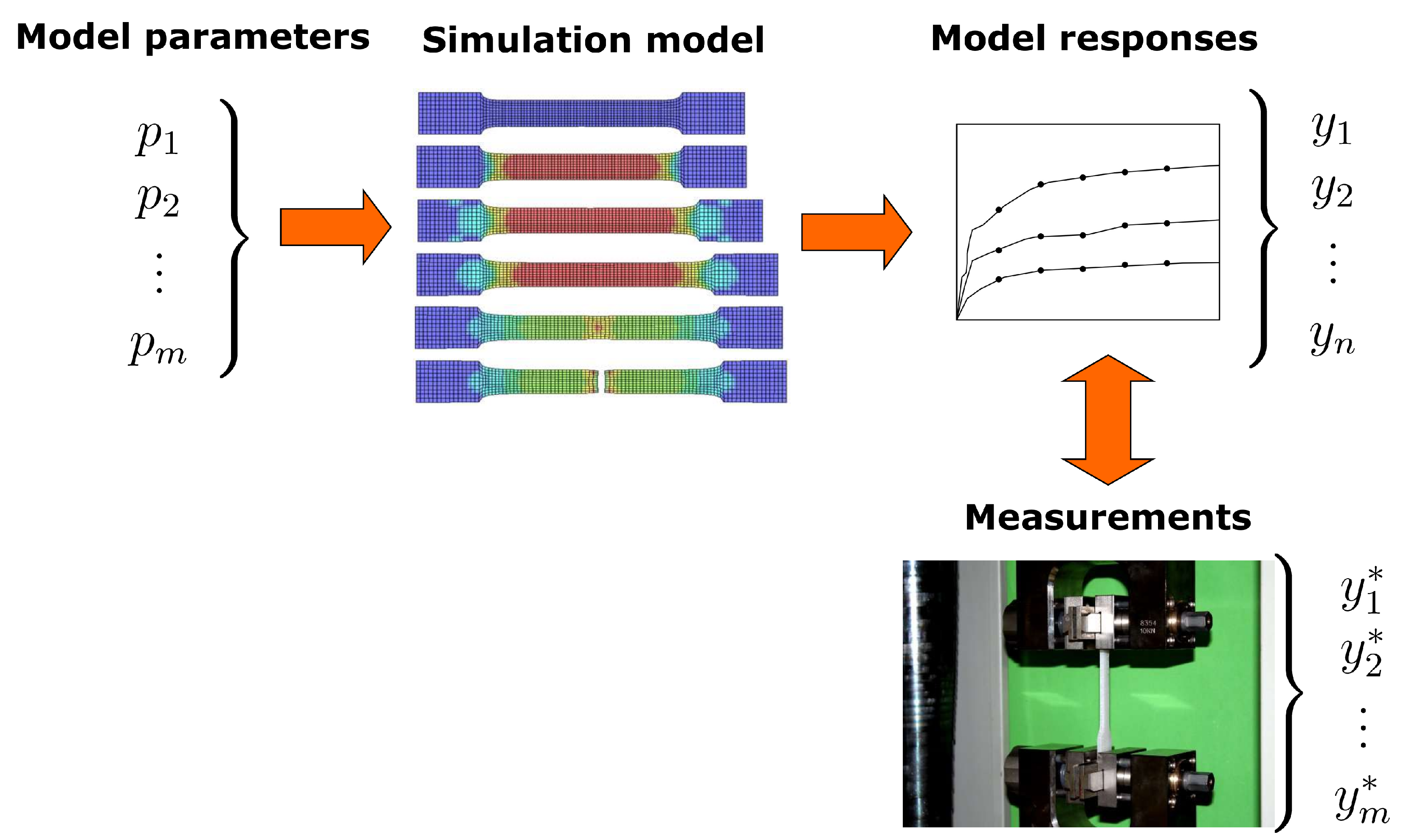
Figure 2.
Bilinear elasto-plasticity model: reference stress-strain curve, synthetic measurements and calibrated model.
Figure 2.
Bilinear elasto-plasticity model: reference stress-strain curve, synthetic measurements and calibrated model.

Figure 3.
Bilinear model: scatter and correlations of the calibrated optimal parameters from 1000 samples of noisy measurement points.
Figure 3.
Bilinear model: scatter and correlations of the calibrated optimal parameters from 1000 samples of noisy measurement points.
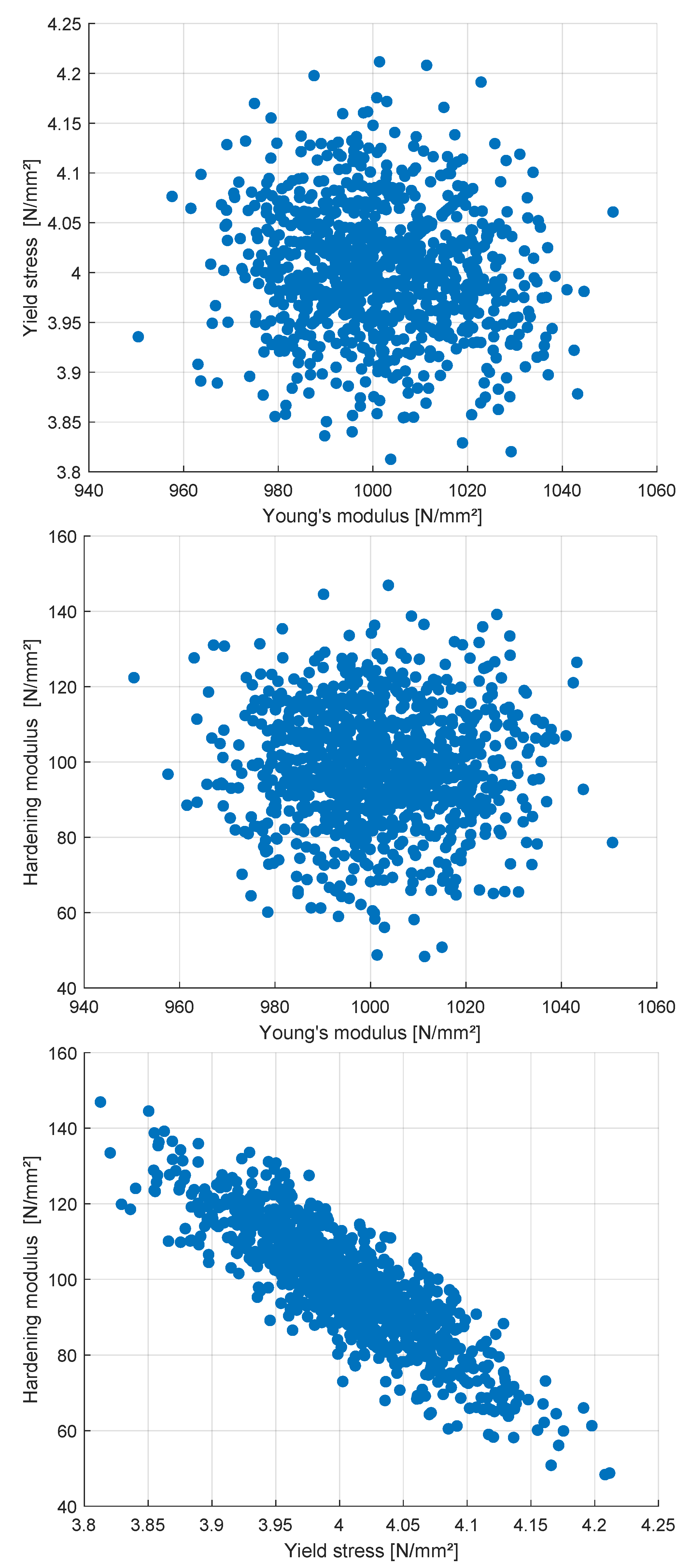
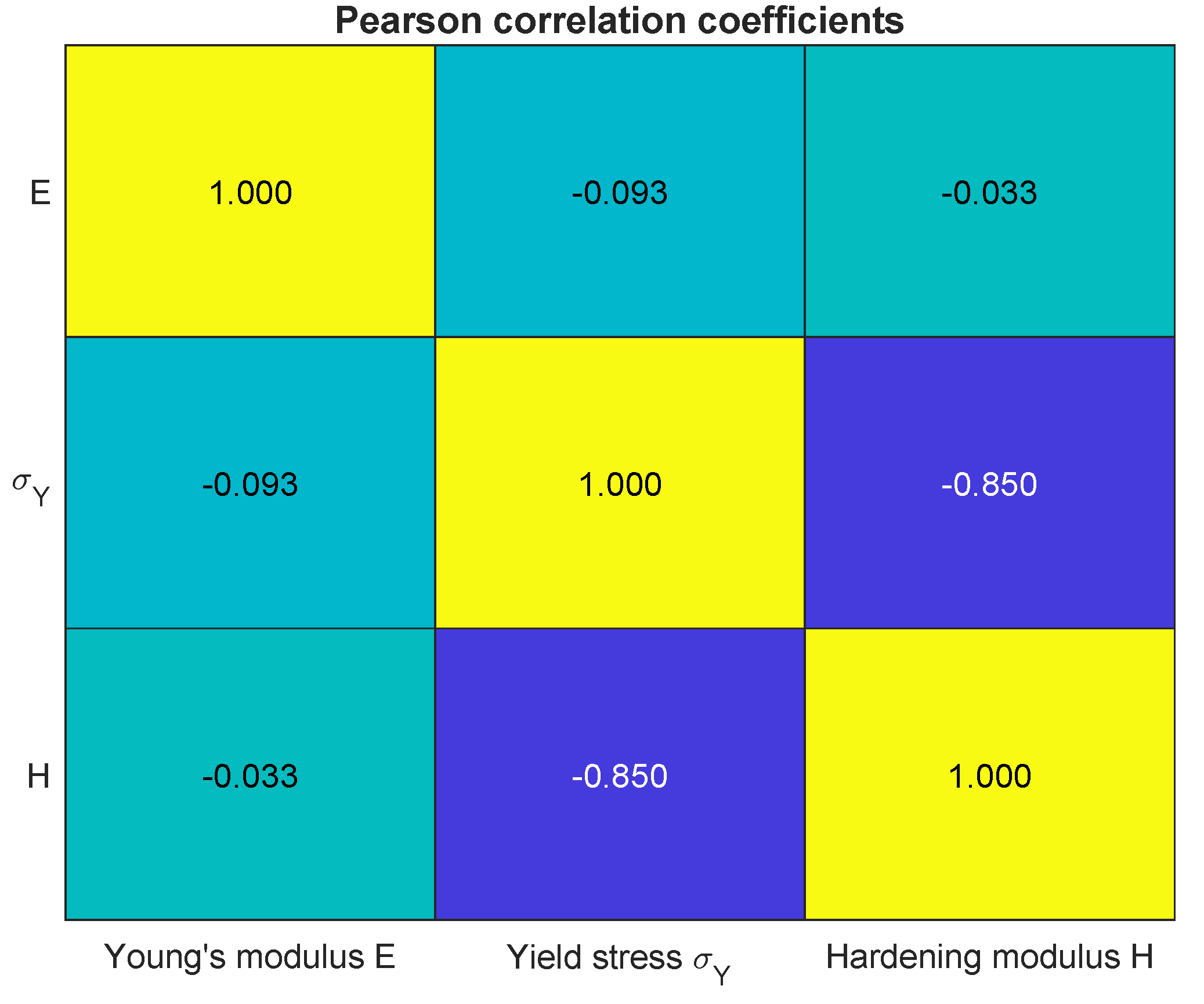
Figure 4.
Bilinear model: approximated first order sensitivity indices using squared correlation coefficients (left) and total effect sensitivity indices using the Metamodel of Optimal Prognosis [33] (right) from 1000 Latin Hypercube samples
Figure 4.
Bilinear model: approximated first order sensitivity indices using squared correlation coefficients (left) and total effect sensitivity indices using the Metamodel of Optimal Prognosis [33] (right) from 1000 Latin Hypercube samples
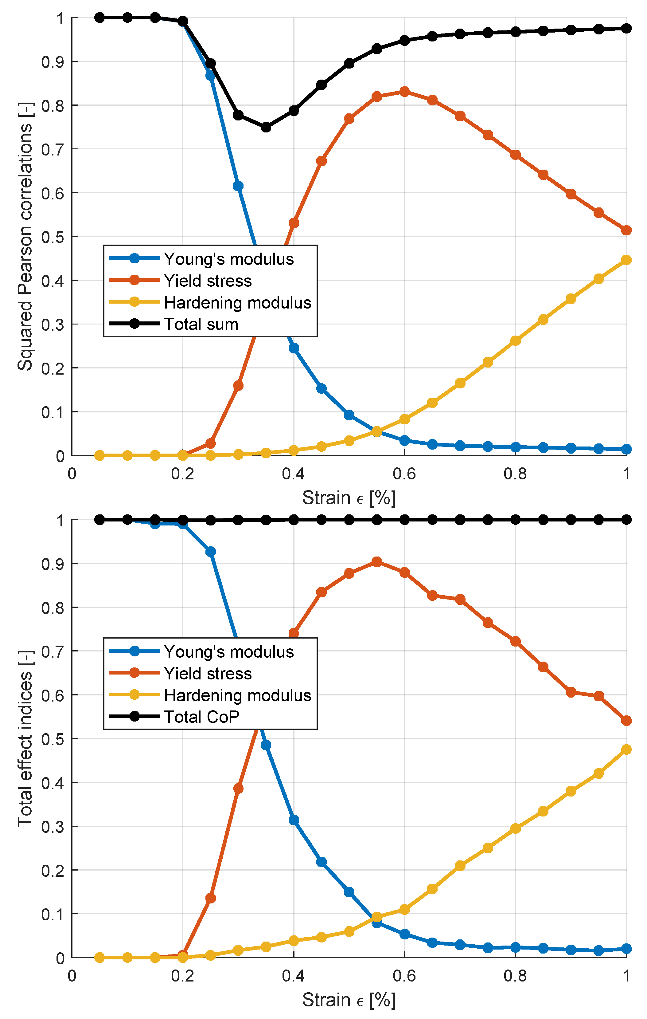
Figure 5.
Bilinear model: estimated parameter scatter by using the Markov estimator with 20 measurement points on the stress-strain curve and independent measurement errors .
Figure 5.
Bilinear model: estimated parameter scatter by using the Markov estimator with 20 measurement points on the stress-strain curve and independent measurement errors .
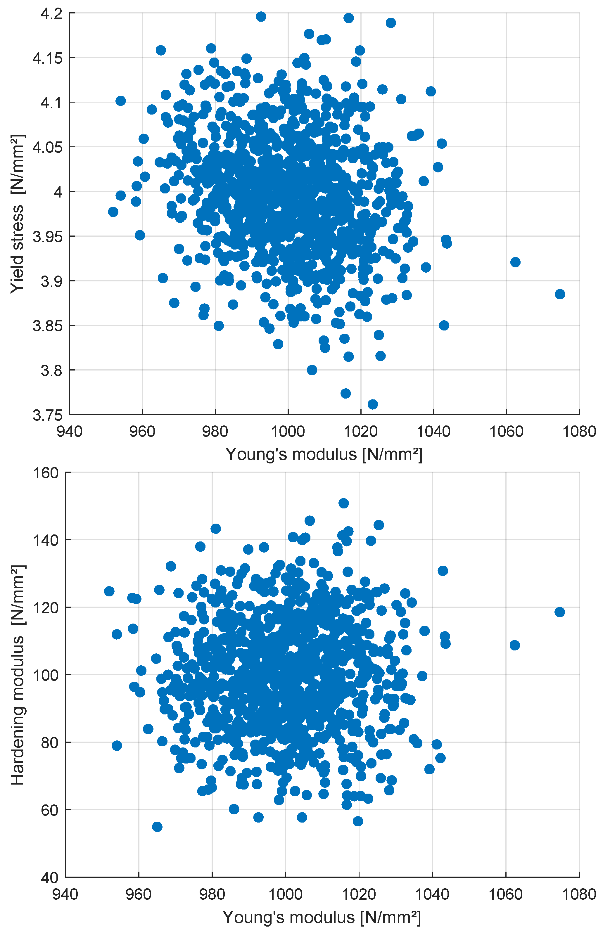
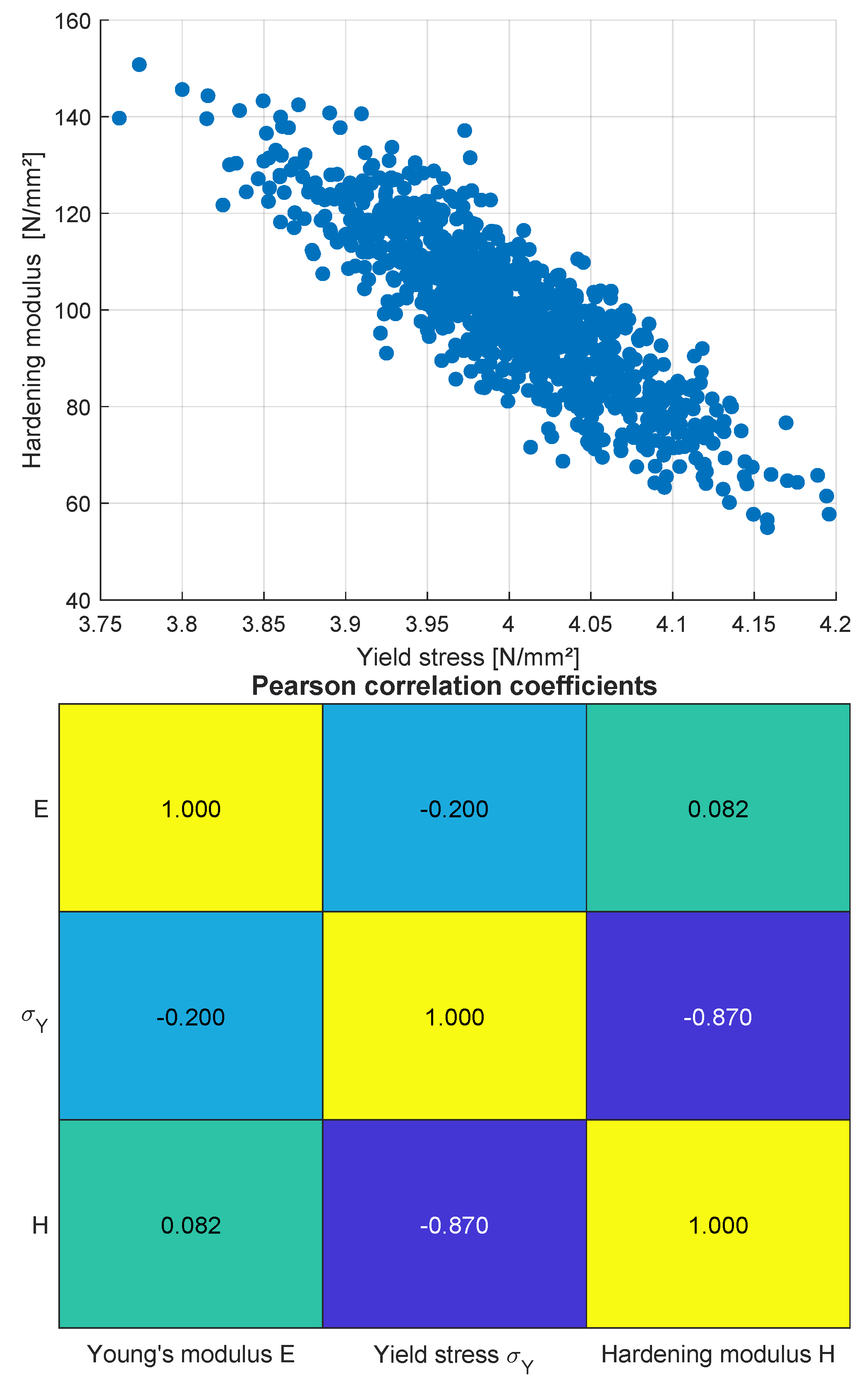
Figure 6.
Bilinear model: normalized partial derivatives at the optimal parameter set (left) and corresponding local first order sensitivity indices (right).
Figure 6.
Bilinear model: normalized partial derivatives at the optimal parameter set (left) and corresponding local first order sensitivity indices (right).
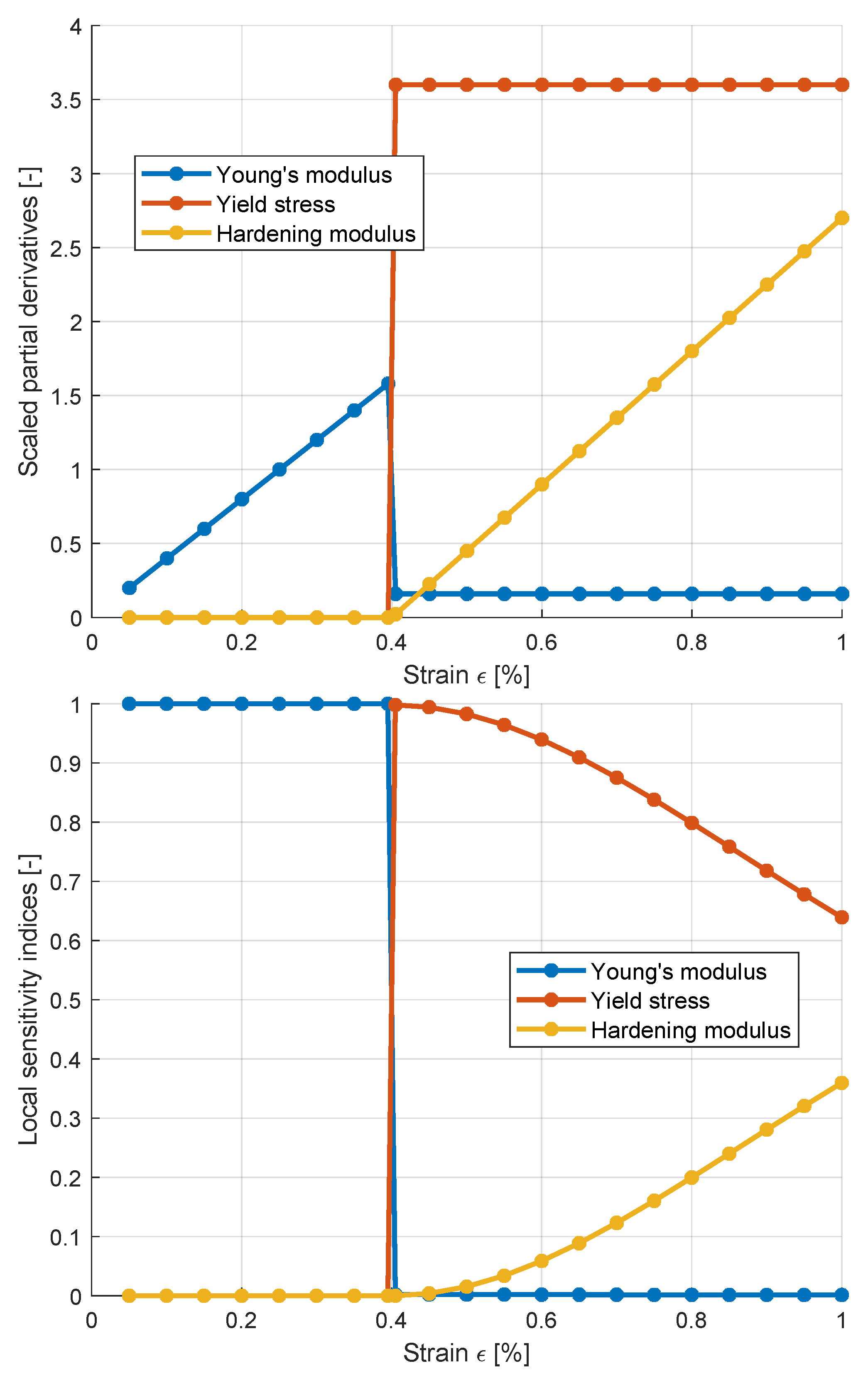
Figure 7.
Bilinear model: estimated parameter scatter normalized with the parameter ranges dependent on the measurement error (left) and dependent on the number of measurement points (right).
Figure 7.
Bilinear model: estimated parameter scatter normalized with the parameter ranges dependent on the measurement error (left) and dependent on the number of measurement points (right).
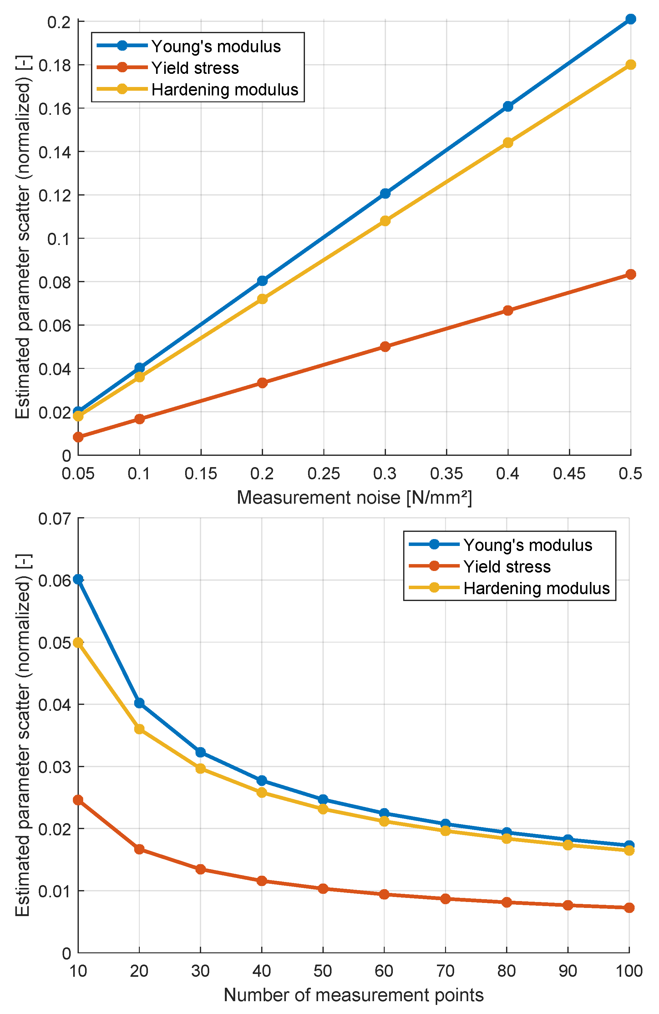
Figure 8.
Bilinear model: estimated parameter scatter by using Bayesian updating with 20 measurement points on the stress-strain curve and independent measurement errors .
Figure 8.
Bilinear model: estimated parameter scatter by using Bayesian updating with 20 measurement points on the stress-strain curve and independent measurement errors .
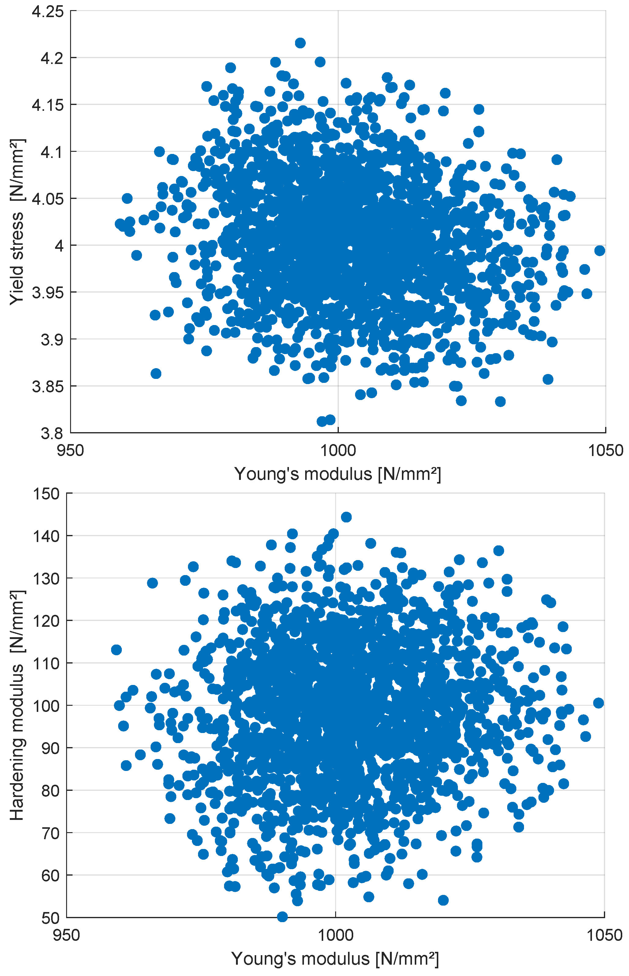
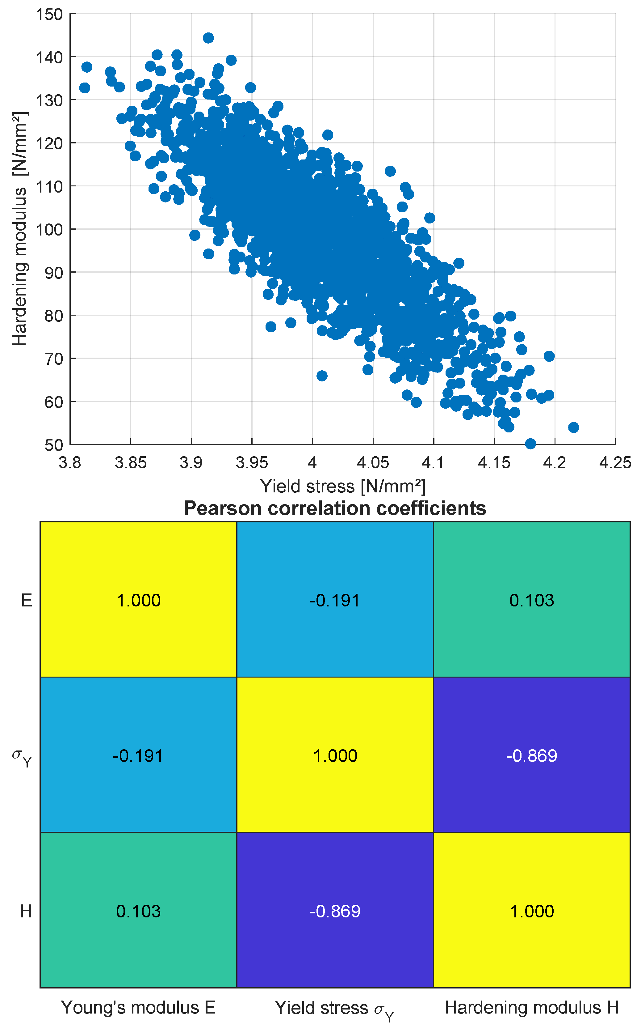
Figure 9.
Bilinear model: Estimated response statistics of Bayesian parameter samples by assuming independent measurement errors with .
Figure 9.
Bilinear model: Estimated response statistics of Bayesian parameter samples by assuming independent measurement errors with .
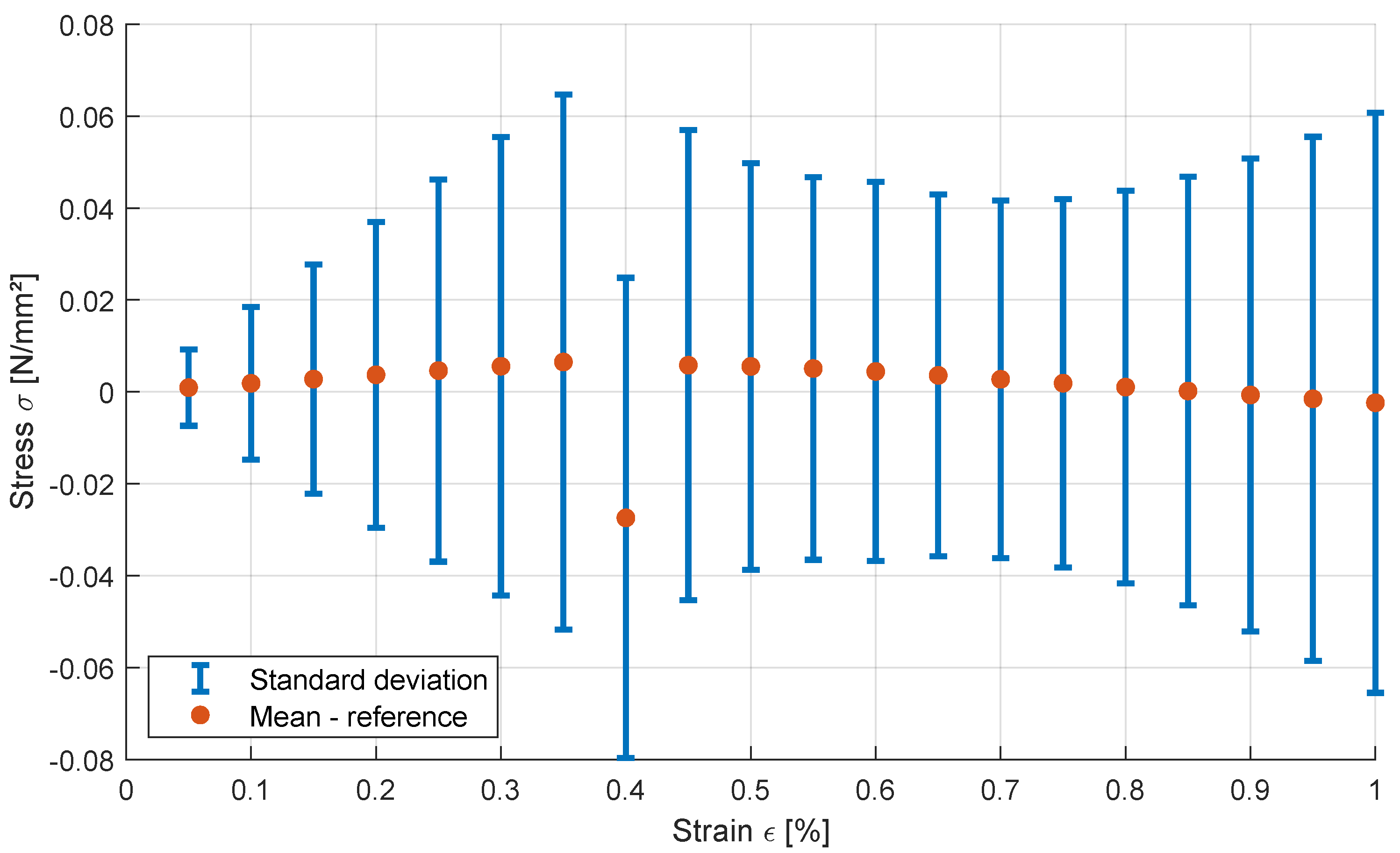
Figure 10.
Interval optimization as inverse identification of minimum and maximum parameter bounds based on given measurement intervals.
Figure 10.
Interval optimization as inverse identification of minimum and maximum parameter bounds based on given measurement intervals.
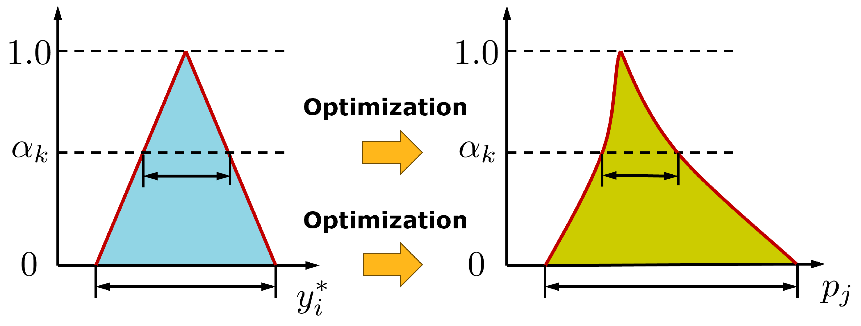
Figure 11.
Bilinear model: obtained parameter sets for the minimization and maximization of the Young’s modulus (blue), the yield stress (red) and the hardening modulus (green) considering a measurement interval of .
Figure 11.
Bilinear model: obtained parameter sets for the minimization and maximization of the Young’s modulus (blue), the yield stress (red) and the hardening modulus (green) considering a measurement interval of .
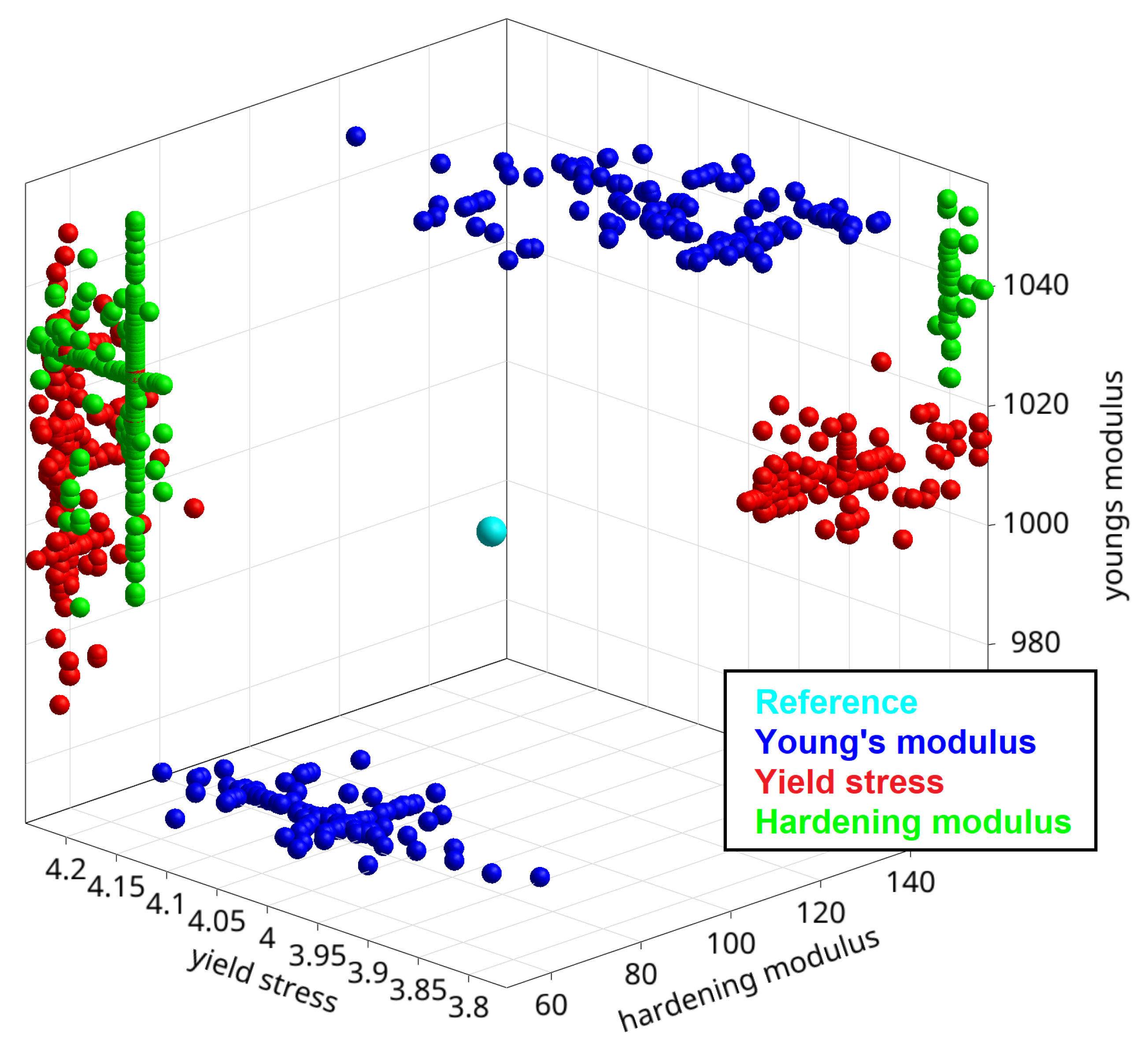
Figure 12.
Identification of the feasible input parameter domain by an radial line-search approach.
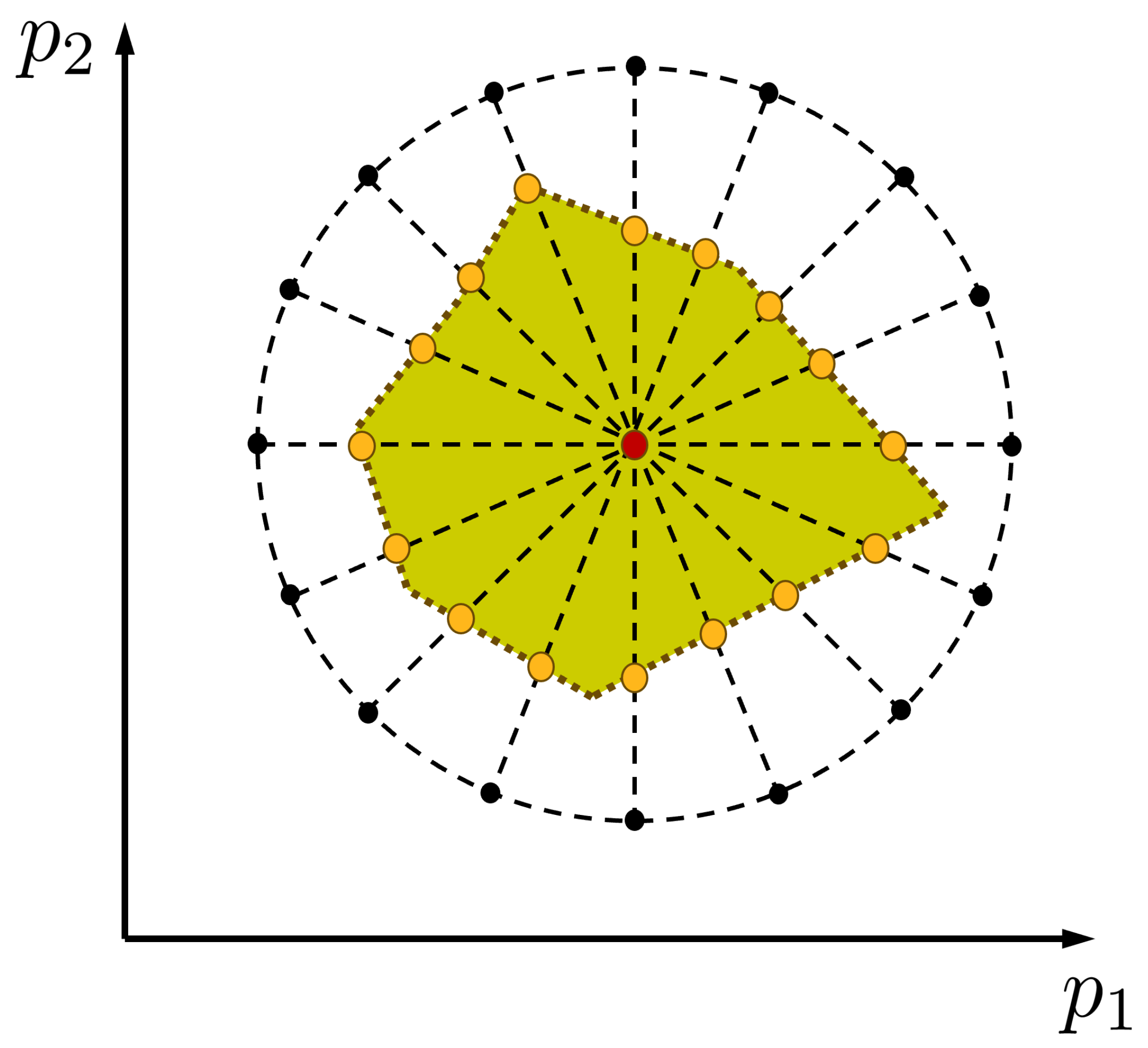
Figure 13.
Bilinear model: obtained parameter bounds from the radial line-search approach in the 2D subspaces of the Young’s modulus, yield stress and hardening modulus considering a measurement interval of .
Figure 13.
Bilinear model: obtained parameter bounds from the radial line-search approach in the 2D subspaces of the Young’s modulus, yield stress and hardening modulus considering a measurement interval of .
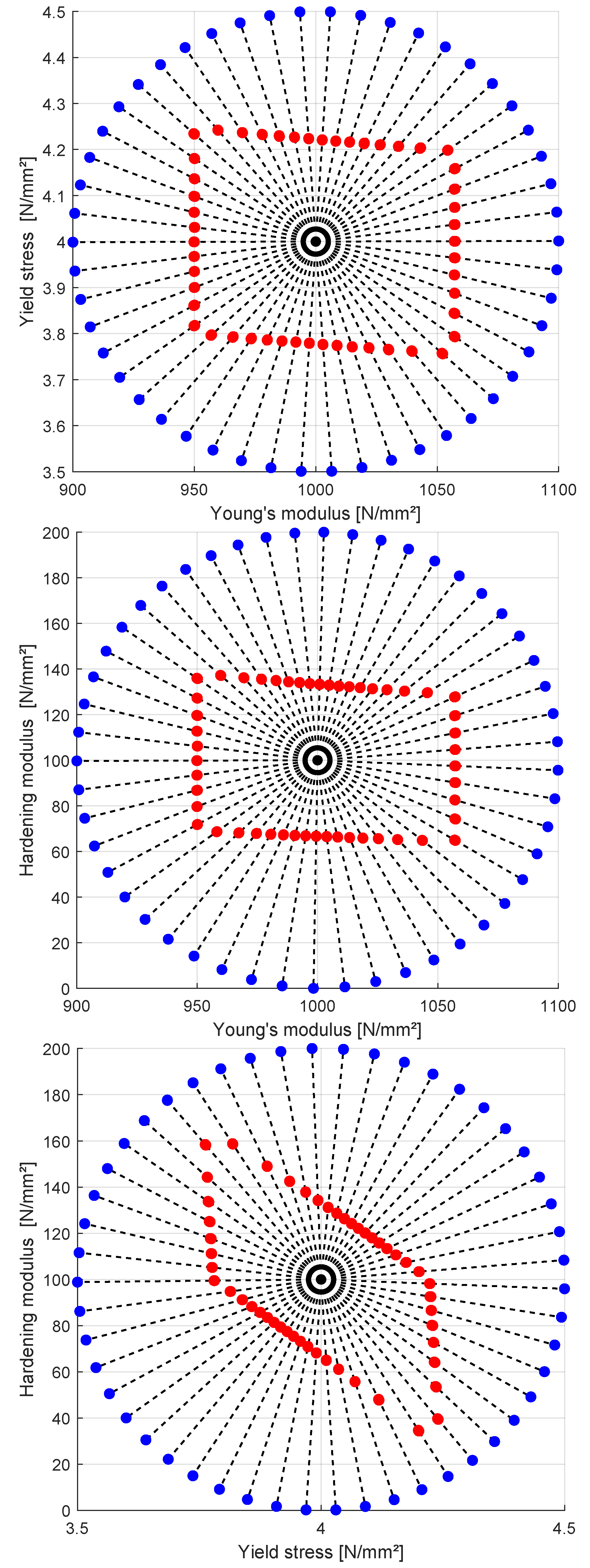
Figure 14.
Bilinear model: 500 initial Fekete points (left) and final line-search points on the boundary of the feasible parameter domain (right) by considering .
Figure 14.
Bilinear model: 500 initial Fekete points (left) and final line-search points on the boundary of the feasible parameter domain (right) by considering .
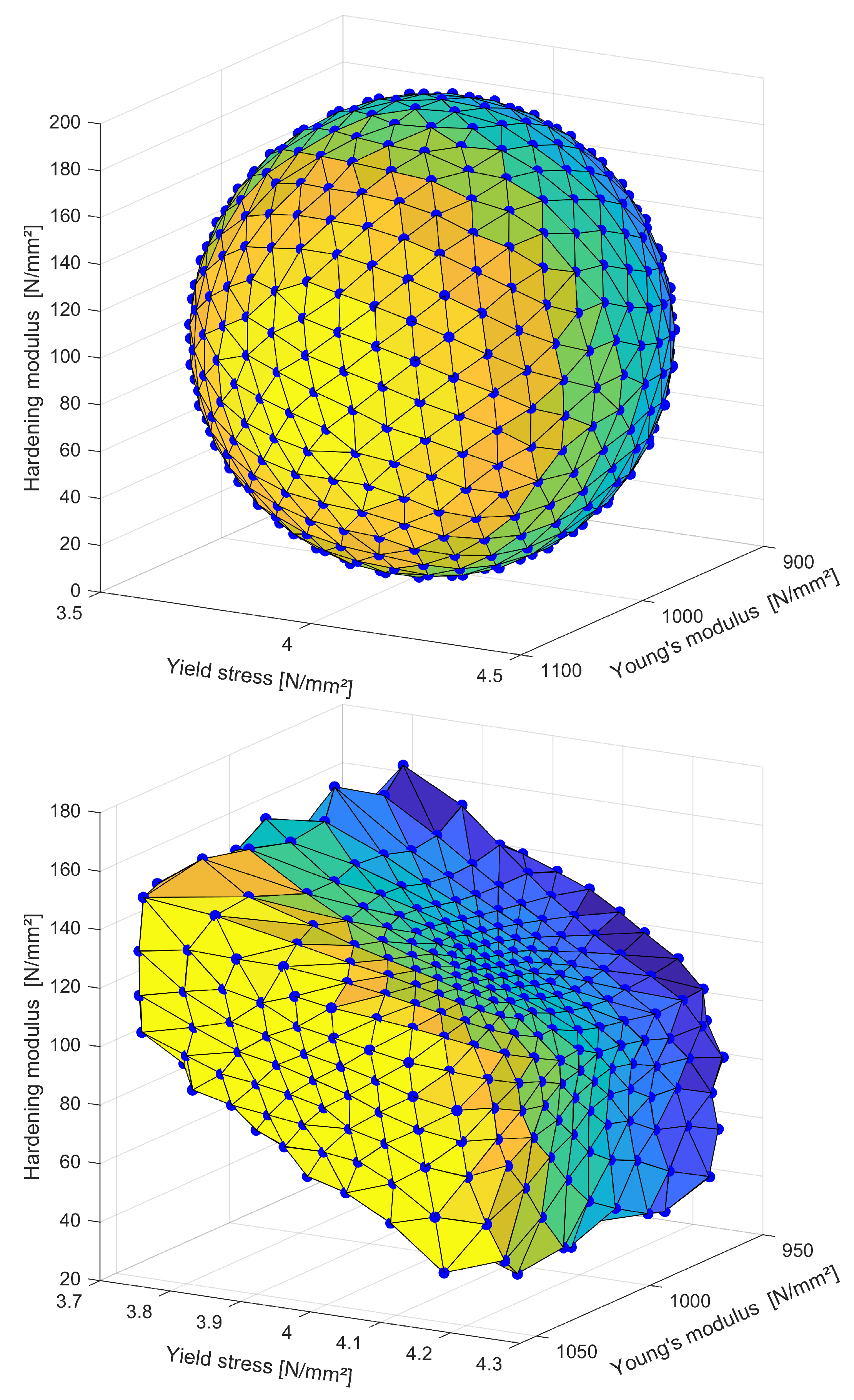
Figure 15.
Bilinear model: obtained response ranges of the three parameter line-search considering a measurement interval of .
Figure 15.
Bilinear model: obtained response ranges of the three parameter line-search considering a measurement interval of .
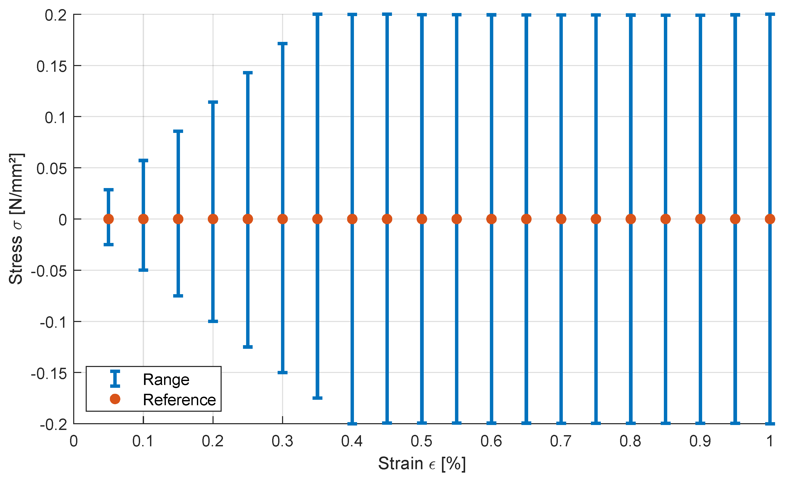
Figure 16.
Wedge splitting test: geometry, bi-linear softening law and finite element model with 2D plane-stress elements and interface elements as predefined crack.
Figure 16.
Wedge splitting test: geometry, bi-linear softening law and finite element model with 2D plane-stress elements and interface elements as predefined crack.
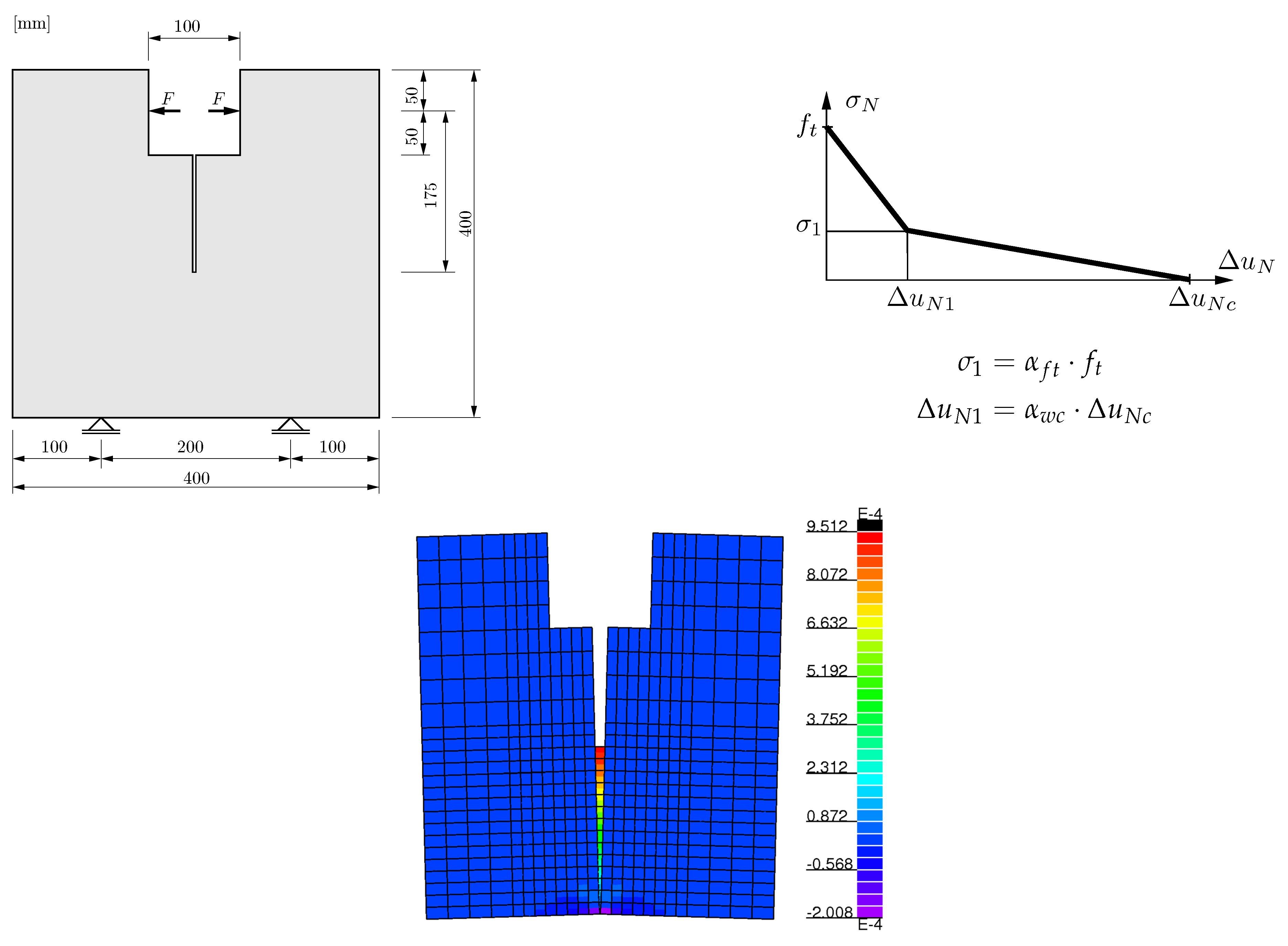
Figure 17.
Wedge splitting test: experimental measurement values and 200 Latin Hybercube samples of the simulated load-displacement curve using the initial parameter bounds.
Figure 17.
Wedge splitting test: experimental measurement values and 200 Latin Hybercube samples of the simulated load-displacement curve using the initial parameter bounds.
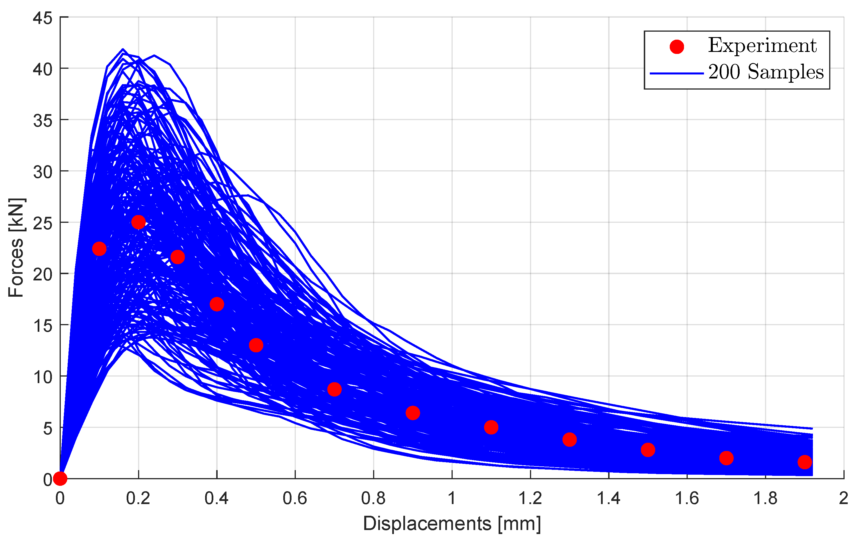
Figure 18.
Wedge splitting test: estimated total effect sensitivity estimates using the Metamodel of Optimal Prognosis.
Figure 18.
Wedge splitting test: estimated total effect sensitivity estimates using the Metamodel of Optimal Prognosis.
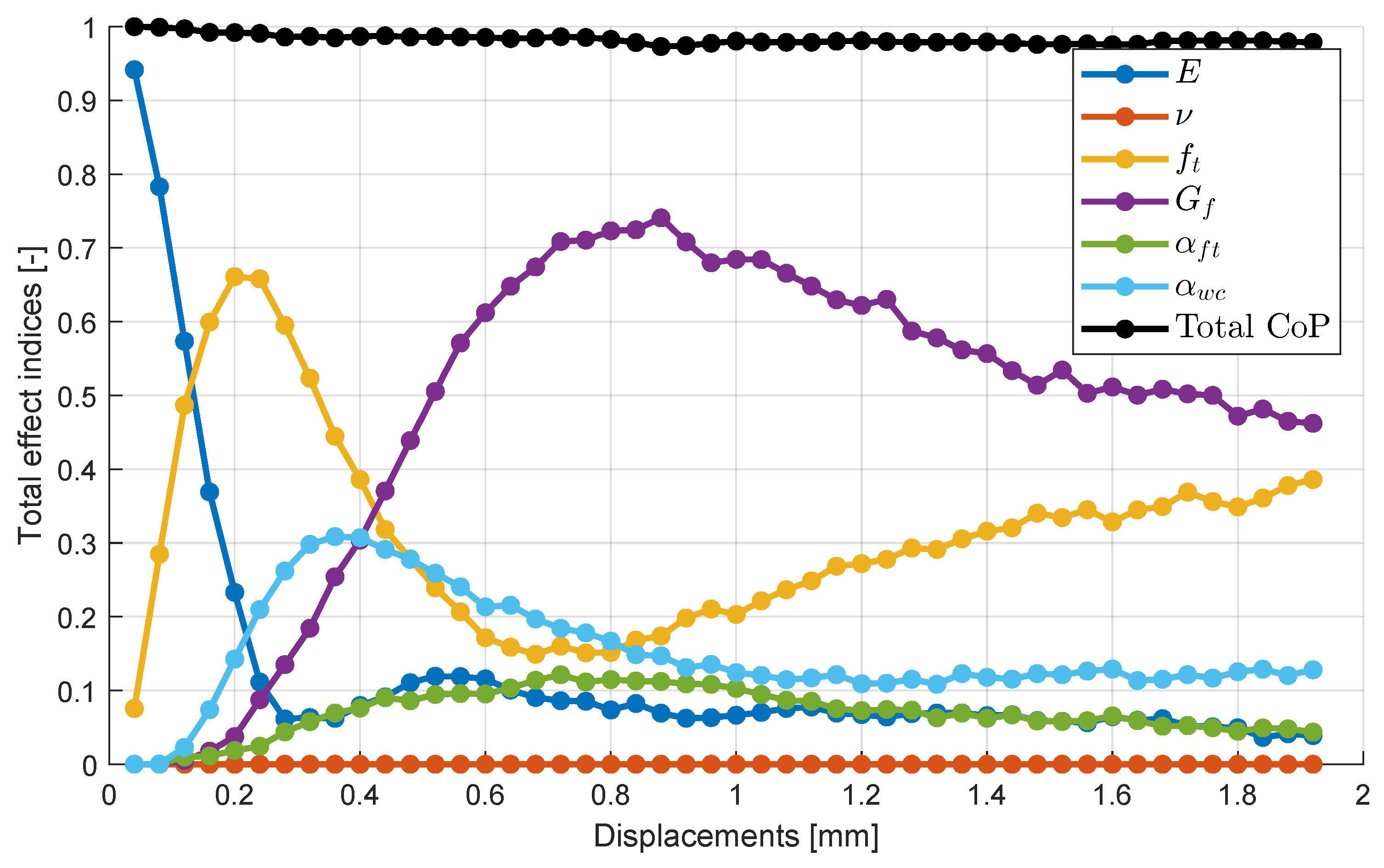
Figure 19.
Wedge splitting test: experimental measurement values compared to the simulated load-displacement curve with optimal parameter values.
Figure 19.
Wedge splitting test: experimental measurement values compared to the simulated load-displacement curve with optimal parameter values.
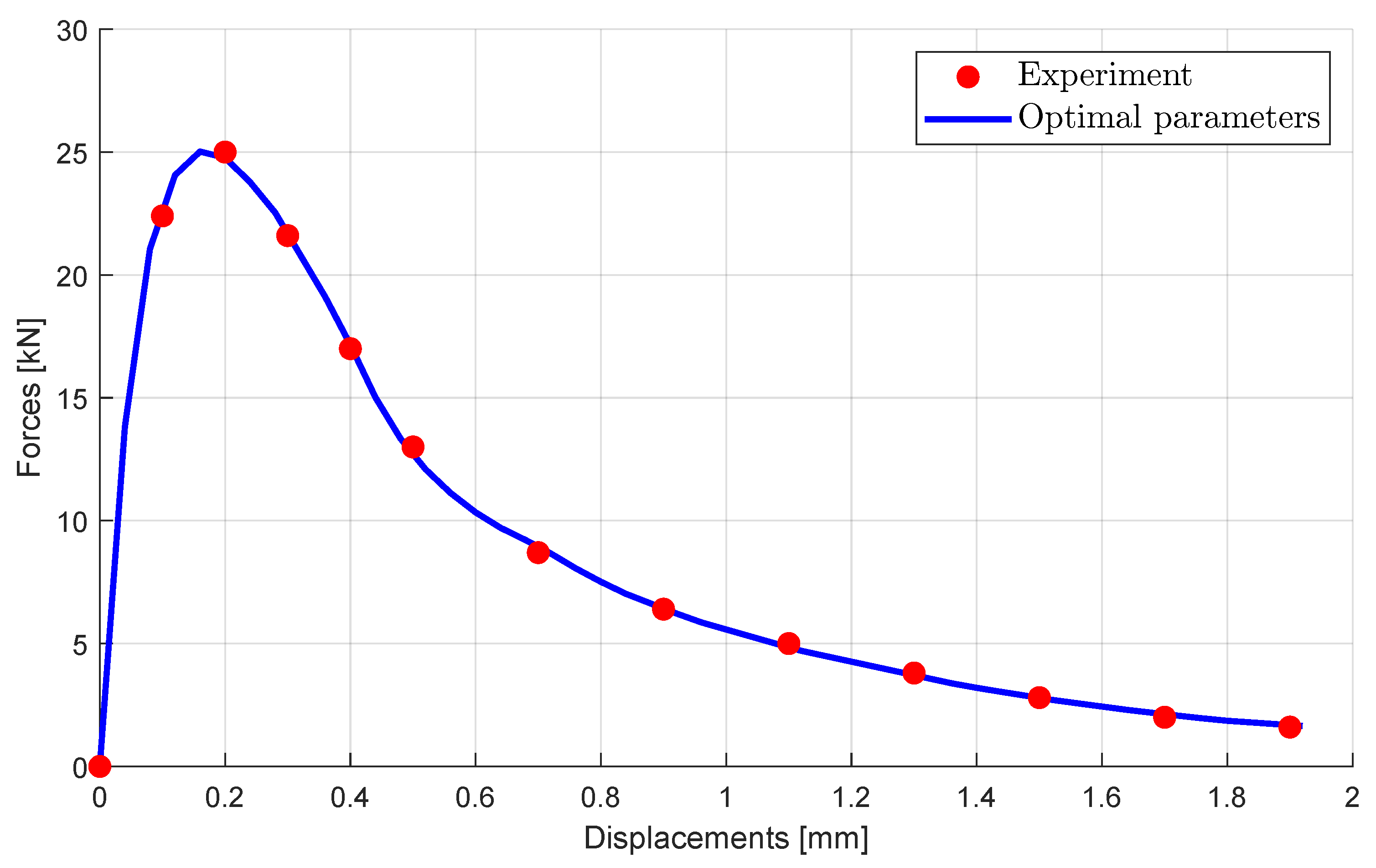
Figure 20.
Wedge splitting test: estimated parameter scatter and correlations using the Markov estimator and Bayesian updating.
Figure 20.
Wedge splitting test: estimated parameter scatter and correlations using the Markov estimator and Bayesian updating.
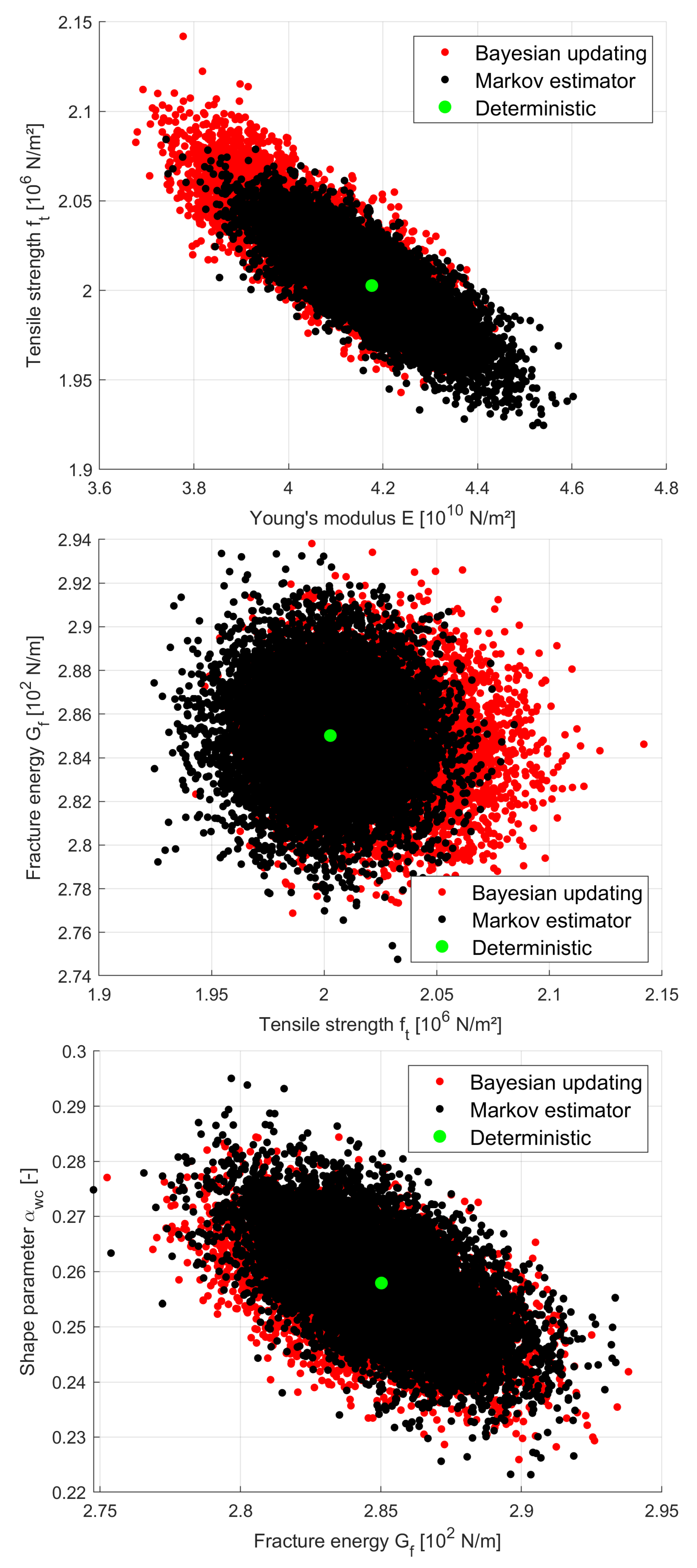
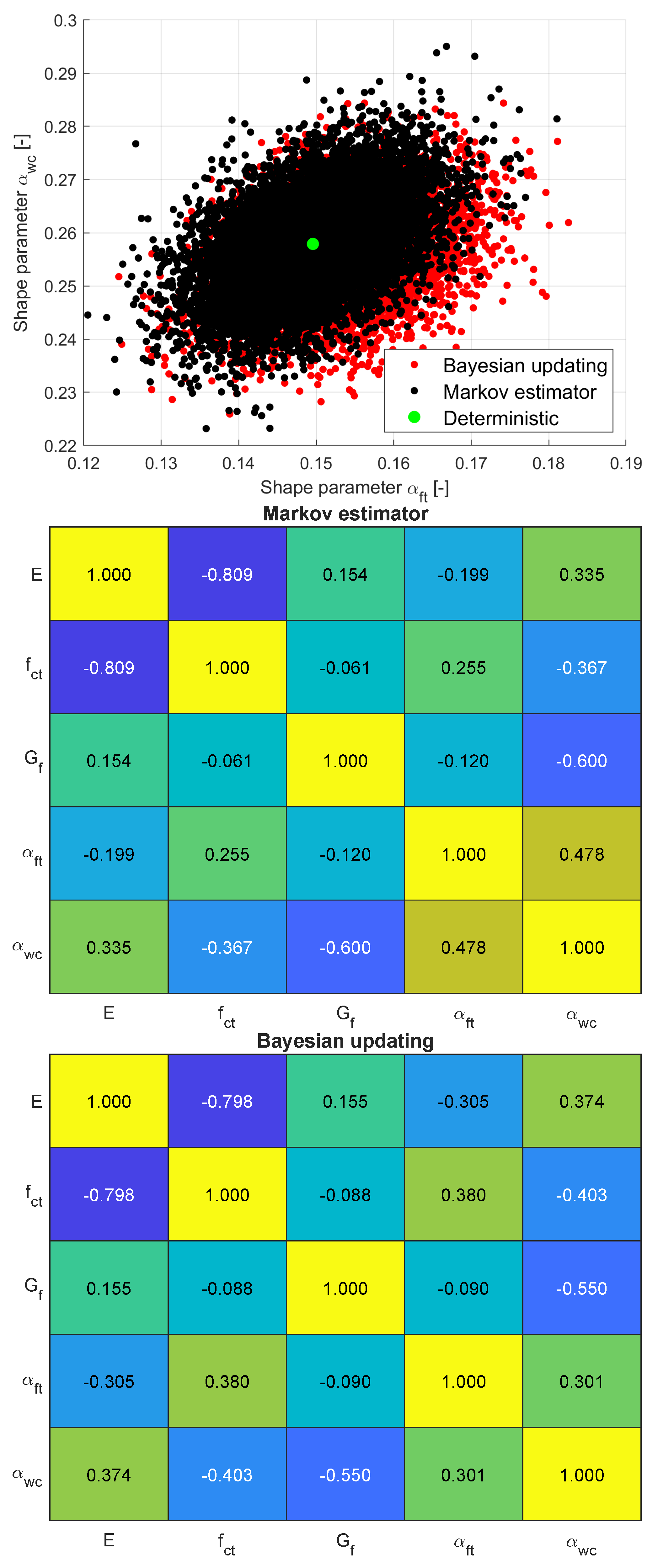
Figure 21.
Wedge splitting test: radial search directions and obtained boundary points for the 2D analysis with (left) and boundary points for different interval sizes (right).
Figure 21.
Wedge splitting test: radial search directions and obtained boundary points for the 2D analysis with (left) and boundary points for different interval sizes (right).
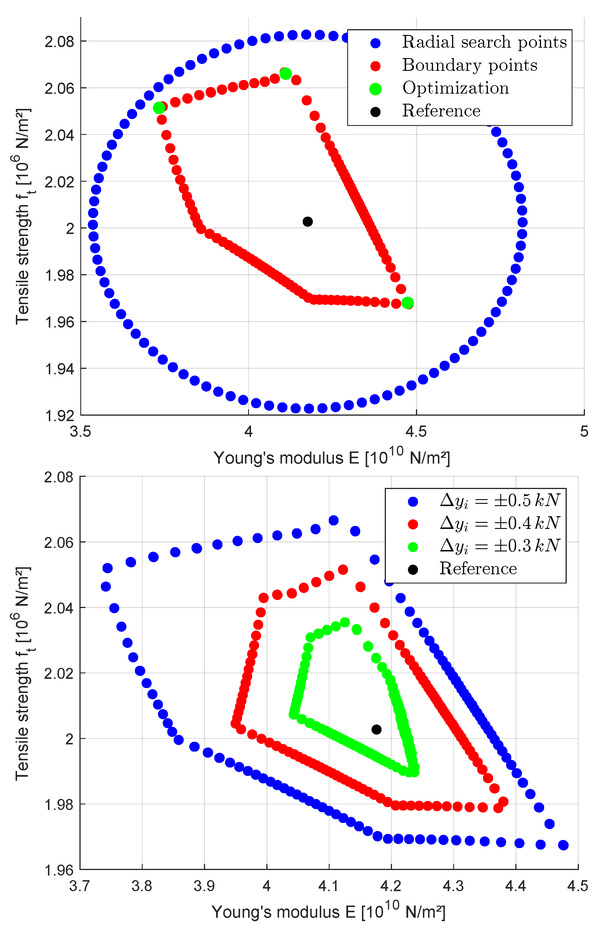
Figure 22.
Wedge splitting test: minimum and maximum parameter values determined by interval optimization and the obtained boundary points from the 5D radial line-search approach by using 5.000 directions with .
Figure 22.
Wedge splitting test: minimum and maximum parameter values determined by interval optimization and the obtained boundary points from the 5D radial line-search approach by using 5.000 directions with .
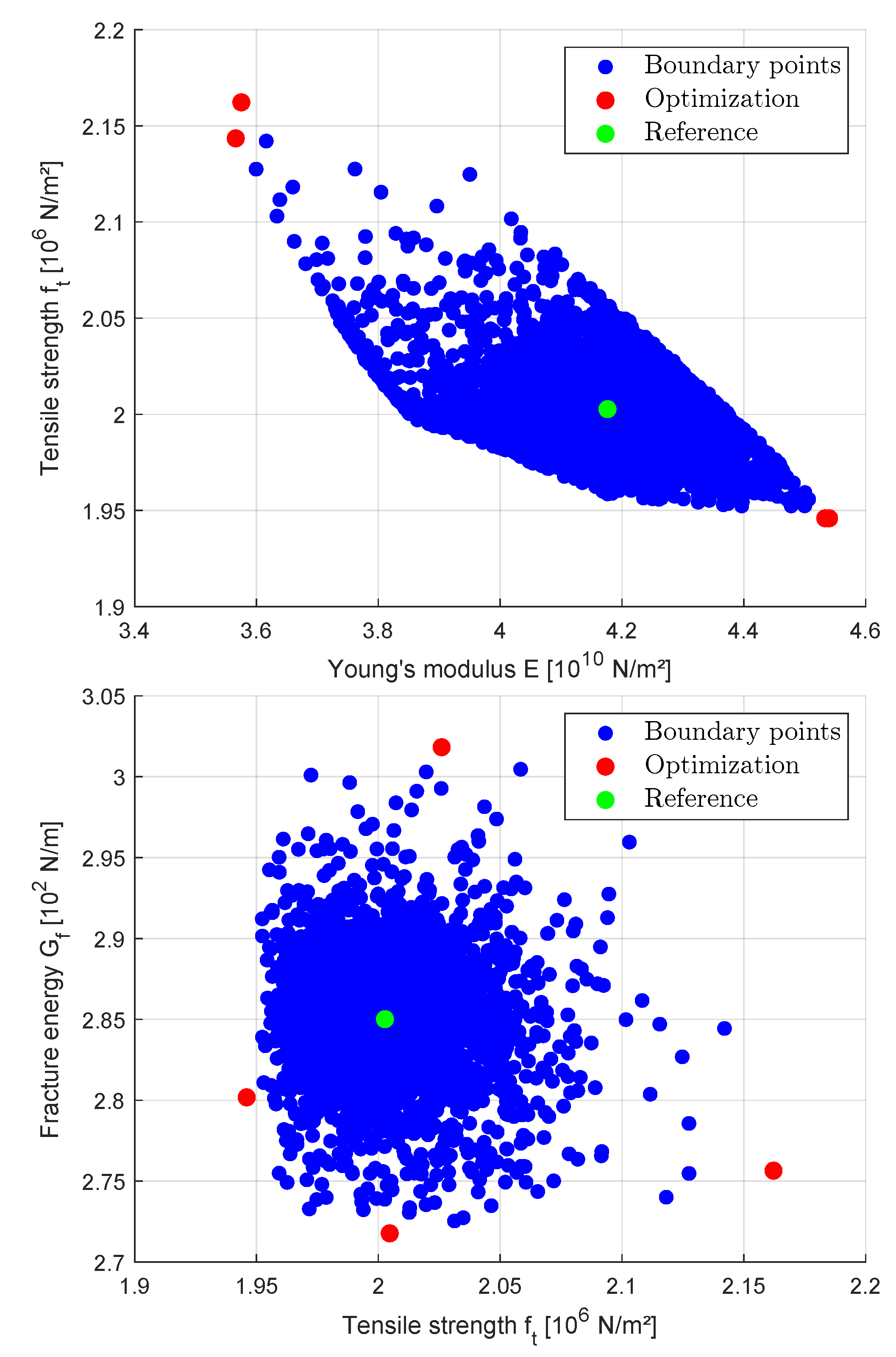
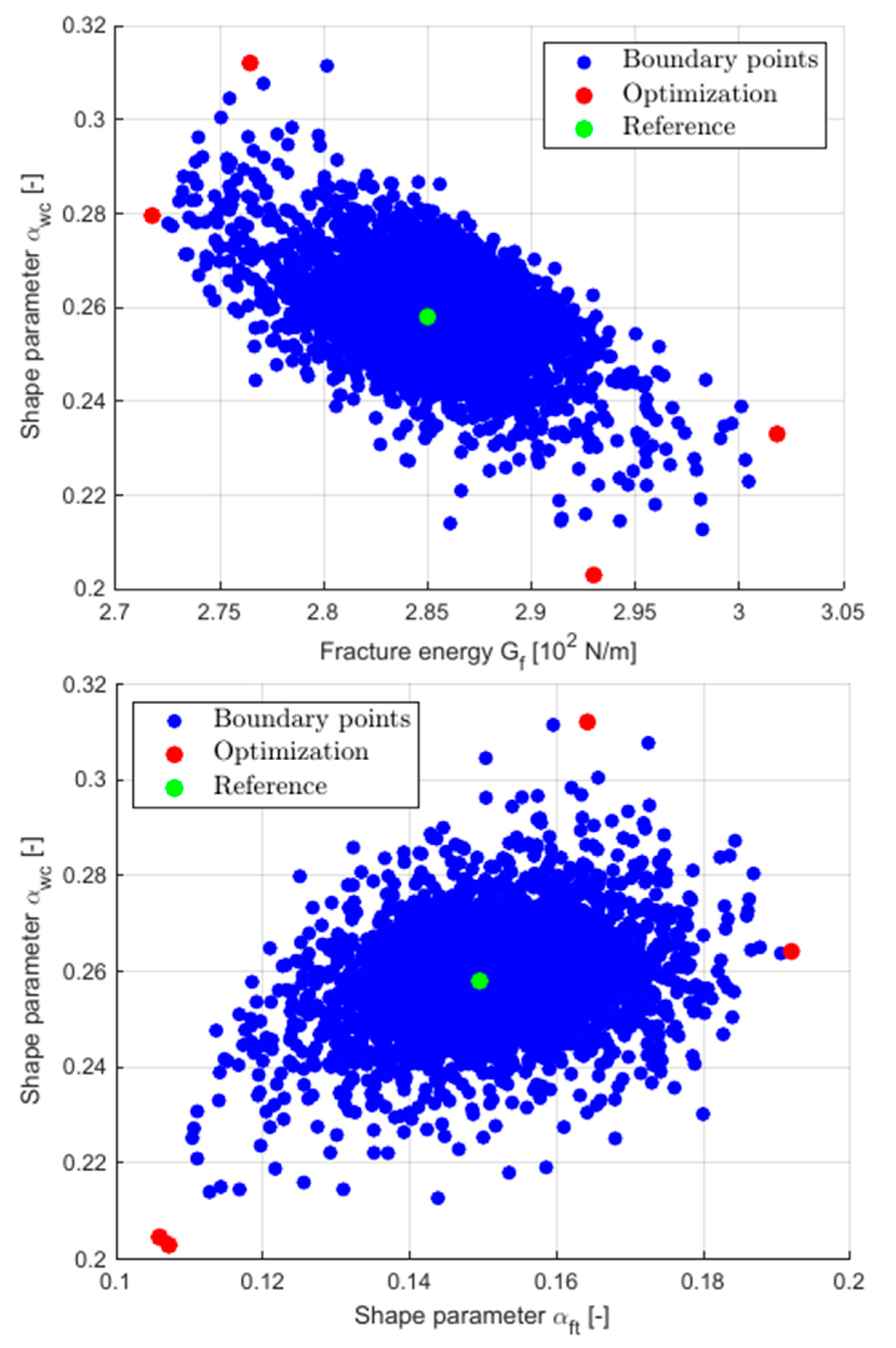

Table 1.
Wedge splitting test: initial material parameter bounds and optimal values.
| Parameter | Unit | Reference value | Bounds | Deterministic optimization | |
|---|---|---|---|---|---|
| Young’s modulus E | 2.830 | 1.00 - 6.00 | 4.176 | ||
| Poisson’s ratio | − | 0.180 | 0.10 - 0.40 | - | |
| Tensile strength | 2.270 | 1.00 - 4.00 | 2.003 | ||
| Fracture energy | 2.850 | 2.00 - 4.00 | 2.850 | ||
| Shape parameter | − | 0.163 | 0.05 - 0.50 | 0.150 | |
| Shape parameter | − | 0.242 | 0.05 - 0.50 | 0.258 | |
Table 2.
Wedge splitting test: estimated statistical properties of the identified parameters using the Markov estimator and Bayesian updating
Table 2.
Wedge splitting test: estimated statistical properties of the identified parameters using the Markov estimator and Bayesian updating
| Parameter | Unit | Markov estimator | Bayesian updating | |||||
|---|---|---|---|---|---|---|---|---|
| Mean | Stddev | CoV | Mean | Stddev | CoV | |||
| Young’s modulus E | 4.176 | 0.116 | 0.028 | 4.065 | 0.136 | 0.033 | ||
| Tensile strength | 2.003 | 0.023 | 0.011 | 2.025 | 0.030 | 0.015 | ||
| Fracture energy | 2.850 | 0.024 | 0.008 | 2.847 | 0.026 | 0.009 | ||
| Shape parameter | − | 0.150 | 0.008 | 0.051 | 0.153 | 0.008 | 0.055 | |
| Shape parameter | − | 0.258 | 0.009 | 0.034 | 0.256 | 0.009 | 0.035 | |
Table 3.
Wedge splitting test: parameter bounds in the 5D parameter space obtained with the interval optimization and defined ranges for the radial line-search approach
Table 3.
Wedge splitting test: parameter bounds in the 5D parameter space obtained with the interval optimization and defined ranges for the radial line-search approach
| Parameter | Unit | Reference | Optimization | Line-search ranges | |||
|---|---|---|---|---|---|---|---|
| Min | Max | ||||||
| Young’s modulus E | 4.176 | 3.566 | 4.540 | ± 1.200 | |||
| Tensile strength | 2.003 | 1.946 | 2.162 | ± 0.176 | |||
| Fracture energy | 2.850 | 2.718 | 3.018 | ± 0.240 | |||
| Shape parameter | − | 0.150 | 0.106 | 0.192 | ± 0.080 | ||
| Shape parameter | − | 0.258 | 0.203 | 0.312 | ± 0.080 | ||
Disclaimer/Publisher’s Note: The statements, opinions and data contained in all publications are solely those of the individual author(s) and contributor(s) and not of MDPI and/or the editor(s). MDPI and/or the editor(s) disclaim responsibility for any injury to people or property resulting from any ideas, methods, instructions or products referred to in the content. |
© 1996 by the author. Licensee MDPI, Basel, Switzerland. This article is an open access article distributed under the terms and conditions of the Creative Commons Attribution (CC BY) license (https://creativecommons.org/licenses/by/4.0/).
Copyright: This open access article is published under a Creative Commons CC BY 4.0 license, which permit the free download, distribution, and reuse, provided that the author and preprint are cited in any reuse.


