
Submitted:
24 December 2024
Posted:
24 December 2024
You are already at the latest version
Abstract
Accurately assessing weevil damage is critical when evaluating banana germplasm to identify genotypes resistant to the banana weevil (Cosmopolites sordidus), for use as elite parents in the banana breeding pipeline or evaluating breeding products. Visual observation remains the most common phenotyping approach but limited by individual bias. This study investigated the potential of image analyses as precise and objective alternatives for assessing weevil damage on the banana corm. Phenotyping trials were set up as partially replicated (P-rep) designs with 22 tissue culture-generated genotypes raised in pots and infested with banana weevils. At termination, the percentage score of weevil damage to the corms was evaluated by visual observation and image analysis using ImageJ and machine learning. In total, 370 high-quality images were assessed for weevil damage using ImageJ and machine learning. On average, damage scores from visual observation were 5.52% and 3.88% higher than ImageJ and machine learning respectively. There was a proportional trend with visual observation agreeing closely to image analyses for smaller scores and but less for larger scores. The results show that both ImageJ and machine learning exhibited a strong level of agreement and are interchangeable with consistent, reliable, and repeatable measurements. In conclusion, to avoid individual bias and subjectivity arising from visual observation, we recommend the use of either ImageJ or machine learning when scoring weevil damage in the banana corm.
Keywords:
Digital phenotyping
; Damage estimation
; Breeding
; Artificial intelligence
; Genotype selection
Introduction
Banana and plantain (Musa spp.) are economically important as income and food security crops worldwide. However, their production is constrained by several pests, including Cosmopolites sordidus, the banana weevil (Kiggundu, 2000; Gold et al., 2001; Viljoen et al., 2016). Banana weevils may cause significant yield losses of up to 40% in the fourth ratoon cycle (Rukazambuga et al., 1998) and 100% beyond the fourth ratoon cycle (Gold et al., 2004). Weevil damage caused by larval feeding leads to necrosis of corm tissue, resulting in impeded water and nutrient uptake and thus reduced bunch size but also reduced anchorage of weakened plants that often snap prematurely (Rukazambuga et al., 1998; Gold et al., 2001).
The method of scoring damage associated with weevils is through visual estimation of the observed damage using the naked eye, which is converted into a percentage of corm damage in relation to the corm size. Weevil damage was assessed by cutting off the pseudo-stem stump to expose rhizome tissue (Gold et al., 2004). The exposed rhizome tissue was examined for weevil larvae damage by dividing the exposed rhizome surface into cross-sections and the number of sections with weevil damage divided by total number of cross sections and multiplied by 100 to calculate the percentage damaged area (Ortiz et al., 1995). Visual observation creates subjectivity that potentially leads to wrong conclusions by over- or underestimation especially when scoring many samples. Accurate and reliable data is essential in crop pathology research and, more so in breeding programs as they serve as the basis to discover susceptibility and resistance levels in breeding germplasm (Li et al., 2020). Thus, there is the need to use high-throughput digital phenotyping tools such as ImageJ or other computer-based tools (Elliot et al., 2022). ImageJ is an open-source Java-written program used in many imaging applications and manipulations to eliminate individual bias and facilitate repeatability and reliability when set ImageJ parameters are kept consistent (Abramoff et al., 2004; Mutka and Bart, 2015; Laflamme et al., 2016; Guiet et al., 2019). ImageJ has mostly been used for quantitative measurements of pest and disease damage on plants, plant growth including height and width, and canopy cover (Stawarczyk and Stawarczyk, 2015; Agehara, 2020). Recent advances in machine learning have further enhanced these capabilities, allowing for more precise and automated analysis of plant health and growth parameters, thereby improving accuracy and efficiency in agricultural research (Kamilaris and Prenafeta-Boldú, 2018; Ubbens and Stavness, 2017; Singh et al., 2016).
Digital methods that provide quicker and more accurate quantification of damage by employing computer algorithms (Lindow and Webb, 1983), can be automated to study a larger number of images at the same time. In addition, it has the ability to automatically distinguish infected tissue from healthy tissue as well as to visualize small damages that may escape the naked eye (Mutka and Bart 2015). The effectiveness of digital data visualization tools is dependent on the ability to take quality images and using them to train the software to accurately classify and capture the phenotypic variation among test genotype samples. Digital detection and quantification tools have mostly been tested for vegetative parts of the diseased plants despite symptoms developing in other parts of the plant as well (Arnal Barbedo, 2013; Veerendra et al., 2021). It is important to apply such tools in quantifying disease symptoms in other plant parts such as corms and roots. In this study, we explore the efficiency of image analysis using ImageJ and customized machine learning image-based tool in comparison with visual estimation when scoring weevil damage in the banana corm.
Materials and Methods
1.0. Experimental Setup
The study was conducted at the International Institute of Tropical Agriculture-Sendusu station in Uganda. A hundred and eighty-five tissue culture-generated plants representing 22 genotypes were evaluated in pot trials using a Partially replicated (p-rep) experimental design (Williams et al., 2014). Each genotype was replicated twice with four pseudo replications per genotype per block. Calcutta 4, a known weevil-resistant genotype and three susceptible landraces to include Mbwazirume (Highland cooking banana), Mchare (Highland cooking banana) and Obino lÉwai (plantain) were used as checks. Infestation with three female and three male weevils was at 60 days post-planting upon attainment of sufficient corm size while data collection was at 60 days post-infestation (dpi) following the cross-section method described in Gold et al. (1994).
1.1. Scoring for Weevil Damage Using Visual Observation
The corm was cut transversely, first at the collar (pseudostem and corm juncture) to score upper cross-sectional damage, and two centimeters below the collar to score lower cross-sectional damage. For each cross-section, weevil damage was assessed separately for the central cylinder and the cortex, estimating the percentage of corm tissue damaged by the weevil in each area. The exposed corm was divided into four sections. The total number of sections with weevil damage is divided by four and multiplied by 100 to calculate the percentage of cross-sectional damage. Parameters scored included (a) percentage of outer upper cross-sectional damage (cortex), (b) inner upper cross-sectional damage (central cylinder), (c) outer lower cross-sectional damage (cortex), and (d) inner lower cross-sectional damage (central cylinder). The mean of the four scores was calculated to generate the overall damage.
1.2. Scoring for Weevil Damage Using Image Analysis
1.2.1. Image Capture
Corm sections were prepared as discussed in section 1.1. High-quality images of each section showing the genotype name, block, and plot number were captured with a green background to increase contrast and optimize quality as shown in Figure 1. A ruler was incorporated as a reference in all images to ensure precise measurements using the ImageJ tool in Figure 1. The resulting images were saved as Joint Photographic Expert Group (JPEG) format. For each plant, two images representing upper and lower cross-sections were captured, totaling 370 images from 185 plants of 22 genotypes (Supplementary Table S1)
2.0. Image Processing Using ImageJ
We describe the approach taken to process the captured image data as a preparatory step before analysis by ImageJ.
2.1.1. Automated Background Removal
To facilitate the analysis of the images, the background was removed by using the rembg Python package. To improve image accuracy, the initial dull green background shown in Figure 2A was replaced with a consistent bright green background with a RGB value of 0, 128, 0 as shown in Figure 2B. RGB is an additive color model system representing red, green and blue colors of light used on a digital display screen to reproduce a broad array of colors for sensing and displaying images in electronic systems. The newly generated RGB images were preserved in their original size and saved as JPEG files with a compression quality of 95, ensuring maximum retention of image quality. Compression quality is the level of perfection in digital images achieved through data minimization without degrading image quality.
2.1.2. Differentiating Healthy and Damaged Regions
The rembg processed images were imported into the ilastik version 1.3.0 tool for labelling to train a custom image classifier. This was to create binary segmentations of the healthy and weevil-damaged tissue as well as background from the corm images. We adopted a two-fold training approach combining manual labeling and automated machine learning algorithms to precisely label healthy and weevil-damaged corm sections plus background on a subset of imported images to complete the segmentation framework and create the labelled dataset.
Using the labelled dataset, ilastik was trained to detect patterns and features characteristic of each region, allowing the custom classifier to accurately categorize and yield binary masks for the entire set of rembg-processed images. For the binary masks, each pixel received a value of 0 or 1 to represent healthy and weevil-damaged sections respectively (Figure 3). Upon completion of binary image segmentation, the trained ilastik model was saved for future analyses.
2.1.3. Quantification of Healthy and Weevil-Damaged Sections
For particle analysis differentiation, the imageJ threshold was adjusted using “Set Threshold (2,2) for healthy and (1,1) for weevil-damaged corm tissue in the binary image. To quantify healthy and weevil-damaged tissue within the binary image, precise parameters, i.e., size: pixel² 0 - infinity, circularity: 0.00 - 1.00 were set to acquire area measurements and standard deviation. These adjustments were used to analyze all ilastik-generated binary images.
2.2. Image Processing Using Machine Learning
We describe the approach taken to process the captured image data using machine learning techniques.
2.2.1. Annotations
Corm images were segmented using the YOLO (“You Only Look Once”) version 8 (Reis et al., 2024) deep learning model that classifies image pixels into different classes. YOLO is a lightweight neural network that performs object detection and segmentation of different regions in images. The image labeling was completed using Makesense (https://www.makesese.ai), a web-based annotation tool that supports drawing of annotations on images (Figure 4). Irregular polygons were drawn on the training set of images to map out boundaries of irregular regions and damaged corm sections. The resultant annotations were exported in Common Objects in Context format (COCO format) (Lin et al., 2014) and converted to YOLO txt labels for training corm segmentation using YOLOv8 model (Reis et al., 2024). YOLOv8 is implemented by Ultralytics, an open-source library that enables training and implementation of various neural networks (Jocher et al., 2023).
2.2.2. Model Training
The images were split into train, test and validation sets using 20, 5, and 5 images respectively. The ultralytics module was utilized for hyperparameter tuning during model training, with modifications such as setting model version to YOLOv8-small; image size to 640 x 640 pixels; batch size to 4; and patience for early stopping to 20 epochs. Most parameters were left as default, however, these specific adjustments were made to optimize the training process for the pre-trained YOLOv8-small model to attain good performance with a small dataset and 100 epochs used to fine-tune the banana corm dataset.
2.2.3. Image Detection Using Trained Model
Image segmentation was completed using Intersection Over Union (IOU), which measures overlap between predicted area and ground truth as a ratio of area of intersection to area of union between ground truth and predicted regions. IOU ranges from 0 to 1, with higher values indicating better predictions. This metric was used to assess model accuracy when predicting regions in an image belonging to a certain class by comparing the overlap between predicted and ground truth regions (Figure 5). The sum of precisions across different levels of prediction confidence and IOU were used to calculate mean Average Precision (mAP). A value of 0.995 indicated a near perfect segmentation performance on the validation set at mAP0.5 (Figure 6).
2.2.4. Background Removal
To remove the background from the images, a three-step python script was followed. In step 1 an input image was loaded and passed through the trained machine learning model. In step 2 the model analyzed the image and returned a prediction for the mask representing the corm in the image and in step 3 the predicted mask was combined with the input image to retain only the corm and eliminate the background in the image (Figure 7).
2.2.5. Quantification of Healthy and Weevil-Damaged Sections
After the background removal step, the images contained pixels for only the damaged and healthy sections of the corm. These sections were clustered using a pixel-based thresholding technique that used binary classification to determine whether values were larger or less than 120-threshold value, the optimum to distinguish between damaged and healthy pixels in the corm. The input images were converted to grayscale and blurring transformation to improve the detection of different sections. Two image detection thresholds were used to identify damaged sections in the grayscale images. First, the damaged sections were segmented white and healthy as black to obtain healthy section pixels and in step 2 the healthy was segmented white and damaged as black to obtain damaged section pixels. The healthy and damaged pixels were summed to obtain the entire corm pixels. Percentage damage was calculated following equation 1 below.
2.2.6. Model Deployment
The python script developed in 2.2.4 was deployed to automatically analyze all images in the dataset producing results as comma-separated values. (csv) excel file format.
2.3. Data Analysis
2.3.1. Statistical Analysis
Statistical analyses of the data were conducted using Pandas (McKinney, 2012) and Matplotlib (Hunter, 2007) python libraries. The Pandas library was used to compute means, standard deviations, and mean difference (bias value) using the formulae below:
The mean of each score method was determined using equation 2 below:
where, ∑Weevil damage values representing the sum of all weevil damage values in a particular weevil damage scoring method, either the visual or image analysis methods.
The bias value or mean difference was calculated using equation 3 below
where method A and B are either visual score or image analysis methods.
The standard deviation was computed using equation 4 below:
where ∑ = summation, n = number of data points in the sample, xi = represents each data point, and x̄ = the sample mean.
2.3.2. Assessing Agreement Among Score Methods
The Bland-Altman plot was used to visualize and assess agreement among the three methods. The upper and lower limits of agreement (LoA) were set at ±1.96 standard deviations to determine the range within which differences among the methods were expected to lie for 95% of observations from the mean difference (Bland and Altman, 1986). The precision of the Bland-Altman LoA is measured in terms of approximate interval width which is twice the value of margin of error or the difference between the upper and lower bounds of confidence interval (Bland and Altman, 1986).
Matplotlib library was used to generate a Bland-Altman plots (Bland and Altman, 1986) with limits of agreement (LoA) computed using equations 3 and 4 below.
Equation 3; Upper limit of agreement (Upper LoA) =.
Equation 4; Lower limit of agreement (Lower LoA) =Where SD_diff = Standard difference
The Numpy library was used to compute the correlation coefficient using equation 5 below:
where X and Y represent values of either visual score or Image analysis score methods; x̅ and ȳ are the means of X and Y, respectively; Σ = the sum of the products and squares over all data points.
Stats model python library was used to compute Lin’s concordance correlation coefficient (CCC) using equation 6 below (Lin, 1989). Lin’s CCC measures both precision and accuracy and ranges from 0 to + 1.
W here r = Pearson correlation coefficient; σx and σy are standard deviations of either visual and ImageJ scoring methods, visual and machine learning scoring methods or ImageJ and machine learning scoring methods respectively; μx and μy means of either visual and ImageJ scoring methods, visual and machine learning scoring methods, or ImageJ and machine learning scoring methods respectively. Interpretation of Lin’s CCC according to McBride et al. (2005) (Table 1)
Matplotlib library was used to plot concordance correlation coefficient scatter plot (Hunter, 2007).
Results
Mean and Standard Deviation Scores for Visual Observation and Image Analysis
Visual observation had the highest mean while ImageJ had the lowest. On the other hand, machine learning had the lowest standard deviation while visual observation had the highest standard deviation (Table 2). These results show that ImageJ and machine learning presented nearly similar results compared to visual observation since their standard deviation was much lower than that of visual observation.
Assessing Agreement Between Visual Observation and Image Analysis
From the Bland-Altman plot, we observed a slightly larger bias of 5.53 between visual observation and ImageJ compared with bias values of 1.64 for machine learning and ImageJ; and 3.88 for visual observation and machine learning methods (Figure 8a-c). The Bland-Altman plot width of agreement for machine learning and ImageJ was narrower suggesting better agreement with less variability in differences compared to that of visual observation and image analysis.
Concordance Correlation Coefficient (CCC)
Lin’s CCC scatter plots between visual observation and image analysis showed a widening variation of score points from the 45° line and forming a narrow band indicating a strong relationship between visual observation and image analysis (Figure 9a-c). We observed a strong CCC value of 0.96 between ImageJ and machine learning compared with 0.89 and 0.87 for visual observation and ImageJ as well as visual observation and machine learning respectively (Table 3). According to McBride et al. (2005), Lin’s CCC between ImageJ and machine learning is substantial compared to that between visual observation and image analysis that is poor (Table 1). However, Pearson’s correlation coefficients were strong between visual observation and image analysis (Table 3).
Mean Separation for Visual Observation and Image Analysis
Table 4 shows analysis of variance (ANOVA) for weevil scoring methods, genotypes and interaction between weevil scoring methods and genotypes. Significant differences were only observed among genotypes (p<0.001) (Table 4, Supplementary Figure 1). Visual observation and image analysis weevil damage scoring methods similarly rated the damage within genotypes hence no significant differences were observed (Table 4). Figure 10 shows response of resistant and susceptible checks to weevil infestation. Fisher’s least significant difference consistently classified susceptible and resistant checks similarly across visual observation and image analysis methods (Figure 10). Mean separation scores from all three scoring methods remained consistent, indicating that response of the checks to banana weevil infestation derived from all three methods is identical.
Discussion
Resistance to banana weevil and hence phenotyping for weevil resistance is currently done by expert estimation (Gold et al.,1994). This approach is slow with personal bias which impacts on data quality, processing speed and reproducibility. We assessed the efficiency of visual observation, ImageJ and machine learning in quantifying banana weevil damage in 125 tissue culture-generated plants representing 22 genotypes. From the 370 images analyzed, the mean and standard deviation values of visual observation were generally 5.52% and 3.88% higher than ImageJ and machine learning respectively. This suggests potential overestimation and wider spread data observations with visual observation.
Lin’s CCC scatter plots and high CCC values suggest that the observed data closely matched the line of perfect concordance, demonstrating both high precision and accuracy for machine learning and ImageJ (Lin, 1989). This suggests a strong level of agreement between ImageJ and machine learning, justifying interchangeable use. However, Lin’s CCC scatter plots for visual observation with image analysis methods indicated proportional bias, suggesting that the relationship between the two methods is not perfectly linear (Lin, 1989). Proportional bias occurs when the discrepancy between the two methods systematically increases or decreases with the magnitude of the measurement (Bland and Altman, 1986; Hazra and Gogtay, 2016). In other words, one method may consistently overestimate, or underestimate compared to the other method as the true values increase or decrease. In this context, the observation of proportional bias between visual observation and image analysis methods indicates that while the methods generally agree, there is a tendency for their agreement to vary depending on the size or scale of the damage. For example, larger values might be more accurately measured by one method over the other or vice versa. This could be due to inherent differences in how each method processes or interprets the data.
Visual observation and Image analysis agreed more closely for smaller damage scores and less closely for larger damage scores. The decrease in agreement between visual observation and image analysis as the magnitude of the score increased could be attributed to measurement error, especially when some segments of the corm are lost due to extensive weevil damage, yet ImageJ and machine learning do not capture this change in corm shape.
Genotypes ranked the same across the three score methods regardless of the scoring method used. We recommend adopting image analysis methods to minimize biases in weevil damage scoring that can occur when different personnel perform weevil assessments. Aside from the need to capture quality images and train the software to distinguish between damaged and healthy tissue, image analysis significantly reduces the time required to analyze large datasets accurately with just a single click. In addition to high precision and accuracy, machine learning processes images every two seconds compared to 30 seconds for ImageJ while it takes approximately 1 minute to score for visual observation. The images and results from ImageJ and machine learning can be used to develop detailed database. Despite the benefits from analysis, it is limited by use of good quality images. This can be solved by using DigiEye, an advanced imaging system that captures high-resolution images under controlled light conditions, to capture corm images for weevil analysis. We piloted the use of DigiEye however the data was not sufficient to include in this publication. DigiEye represents a significant advancement in image analysis technology, offering precision, consistency, and objectivity (Kumah et al., 2019). Despite limitations in terms of cost and technical requirements, the benefits make it a valuable tool in weevil damage scoring, since in addition to capturing the image, it can be used to convert the image into binary and ready for analysis in ImageJ hence reducing the initial steps for converting images to binary using ilastik. Future developments, particularly in AI integration, may further enhance its capabilities and broaden its applications.
In conclusion, we recommend adoption and use of imageJ and machine learning when phenotyping for banana weevil resistance. We are currently exploring use of image analysis to phenotype for nematodes and Fusarium oxysporum sp. cubense race 1 in banana.
Supplementary Materials
The following supporting information can be downloaded at the website of this paper posted on Preprints.org.
Author Contributions
AB and RS conceptualized the idea; GM, GVN, RK, CS and JFT investigated, methodology, software validation, visualization and writing original draft; RS, AB, TS, JNN reviewed and edited manuscript. GVN, RS, TS and JNN supervised the work.
Acknowledgments
This work has been supported by the Roots Tubers and Banana (RTB) project funded by Bill and Mellinda Gates Foundation.
Conflicts of Interest
The authors declare that they have no known competing financial interests or personal relationships that could influence the work reported in this paper.
References
- Abramoff, M.D., Magalhães, P.J. and Ram, S.J. (2004). Image processing with ImageJ. Biophotonics International, 11(7), 36-42.
- Agehara, S. (2020). Simple imaging techniques for plant growth assessment: HS1353, 1/2020. EDIS, 2020(1), 5-5. [CrossRef]
- Arnal Barbedo, J. G. (2013). Digital image processing techniques for detecting, quantifying, and classifying plant diseases. SpringerPlus, 2(1), 1-12. [CrossRef]
- Bland, J.M. and Altman, D. (1986). Statistical methods for assessing agreement between two methods of clinical measurement. The Lancet, 1(8476), 307-310.
- Elliott, K., Berry, J.C., Kim, H. and Bart, R.S. (2022). A comparison of ImageJ and machine learning based image analysis methods to measure cassava bacterial blight disease severity. Plant Methods, 18(1), 86. [CrossRef]
- Gold, C.S., Kagezi, G.H., Night, G. and Ragama, P.E. (2004). The effects of banana weevil, Cosmopolites sordidus, damage on highland banana growth, yield and stand duration in Uganda. Annals of Applied Biology, 145(3), 263-269. [CrossRef]
- Gold, C.S., Pena, J.E. and Karamura, E.B. (2001). Biology and integrated pest management for the banana weevil Cosmopolites sordidus (Germar)(Coleoptera: Curculionidae). Integrated Pest Management Reviews, 6(2), 79-155. [CrossRef]
- Gold, C.S., Speijer, P.R., Karamura, E.B., Tushemereirwe, W.K. and Kashaija, I.N. (1994). Survey methodologies for banana weevil and nematode damage assessment in Uganda. African Crop Science Journal 2, 309-321.
- Guiet, R., Burri, O. and Seitz, A. (2019). Open-source tools for biological image analysis. In: Rebollo, E., Bosch, M. (eds) computer optimized microscopy: Methods and Protocols, 23-37. [CrossRef]
- Hazra, A. and Gogtay, N. (2016). Biostatistics series module 6: correlation and linear regression. Indian Journal of Dermatology, 61(6), p.593. [CrossRef]
- Hunter, John D. (2007). Matplotlib: A 2D Graphics Environment. Computing in Science & Engineering, 9(3), 90-95. [CrossRef]
- Jocher, G., Chaurasia, A. and Qiu, J. (2023). YOLO by Ultralytics (Version 8.0. 0)[Computer software]. YOLO by Ultralytics (Version 8.0. 0)[Computer software]. https://github.com/ultralytics/ultralytics.
- Kamilaris, A. and Prenafeta-Boldú, F.X. (2018). Deep learning in agriculture: A survey. Computers and Electronics in Agriculture, 147, 70-90. [CrossRef]
- Kiggundu, A., Gold, C.S. and Vuylsteke, D., 2000. Response of banana cultivars to banana weevil attack. Uganda Journal of Agricultural Sciences, 5(2), 36-40.
- Kumah, C., Zhang, N., Raji, R.K. and Pan, R. (2019). Color measurement of segmented printed fabric patterns in lab color space from RGB digital images. Journal of Textile Science and Technology, 5(1), 1-18. [CrossRef]
- Laflamme, B., Middleton, M., Lo, T., Desveaux, D. and Guttman, D. S. (2016). Image-based quantification of plant immunity and disease. Molecular Plant-Microbe Interactions, 29(12), 919-924. [CrossRef]
- Li, W., Deng, Y., Ning, Y., He, Z. and Wang, G. L. (2020). Exploiting broad-spectrum disease resistance in crops: from molecular dissection to breeding. Annual Review of Plant Biology, 71, 575-603. [CrossRef]
- Lin, L. (1989). A concordance correlation coefficient to evaluate reproducibility. Biometrics 1989, 45:255-268. [CrossRef]
- Lin, T.Y., Maire, M., Belongie, S., Hays, J., Perona, P., Ramanan, D., Dollár, P. and Zitnick, C.L. (2014). Microsoft coco: Common objects in context. In Computer Vision–ECCV 2014: 13th European Conference, Zurich, Switzerland, September 6-12, 2014, Proceedings, Part V 13 (740-755). Springer International Publishing. [CrossRef]
- Lindow, S. E. and Webb, R. R. (1983). Quantification of foliar plant disease symptoms by microcomputer-digitized video image analysis. Phytopathology, 73(4), 520-524.
- McBride, G. B. (2005). A proposal for Strength-of-Agreement Criteria for Lin’s. Concordance Correlation Coefficient. Hamilton: National Institute of Water & Atmospheric Research Ltd.
- McKinney, W. (2012). Python for data analysis: Data wrangling with Pandas, NumPy, and IPython. “ O’Reilly Media, Inc.”.
- Mutka, A. M. and Bart, R. S. (2015). Image-based phenotyping of plant disease symptoms. Frontiers in Plant Science, 5, 734. [CrossRef]
- Ortiz, R., Vuylsteke, D., Dumpe, B. and Ferris, R.S.B. (1995). Banana weevil resistance and corm hardness in Musa germplasm. Euphytica, 86(2), 95-102. [CrossRef]
- Reis, D., Kupec, J., Hong, J. and Daoudi, A. (2024). Real-time flying object detection with YOLOv8. arXiv preprint arXiv:2305.09972. [CrossRef]
- Rukazambuga, N. D. T. M., Gold, C. S. and Gowen, S. R. (1998). Yield loss in East African highland banana (Musa spp., AAA-EA group) caused by the banana weevil, Cosmopolites sordidus Germar. Crop Protection, 17(7), 581-589. [CrossRef]
- Singh, A., Ganapathysubramanian, B., Singh, A.K. and Sarkar, S. (2016). Machine learning for high-throughput stress phenotyping in plants. Trends in Plant Science, 21(2), 110-124. [CrossRef]
- Stawarczyk, M. and Stawarczyk, K. (2015). Use of the ImageJ program to assess the damage of plants by snails. Chemistry-Didactics-Ecology-Metrology, 20(1-2), 67-73. [CrossRef]
- Ubbens, J.R. and Stavness, I. (2017). Deep plant phenomics: a deep learning platform for complex plant phenotyping tasks. Frontiers in Plant Science, 8, 1190. doi: . [CrossRef]
- Veerendra, G., Swaroop, R., Dattu, D. S., Jyothi, C. A. and Singh, M. K. (2021). Detecting plant Diseases, quantifying and classifying digital image processing techniques. Materials Today: Proceedings, 51, 837-841. [CrossRef]
- Viljoen, A., Mahuku, G., Massawe, C., Ssali, R.T., Kimunye, J., Mostert, G., Ndayihanzamaso, P. and Coyne, D.L. (2016). Banana pests and diseases: field guide for disease diagnostics and data collection. International Institute of Tropical Agriculture: Ibadan, Nigeria.
- Williams, E. R., John, J. A. and Whitaker, D. (2014). Construction of more Flexible and Efficient P–rep Designs. Australian & New Zealand Journal of Statistics, 56(1), 89-96. [CrossRef]
Figure 1.
A high-quality image captured for image analysis. Brown areas show damage from the banana weevil (0.6X magnification).
Figure 1.
A high-quality image captured for image analysis. Brown areas show damage from the banana weevil (0.6X magnification).
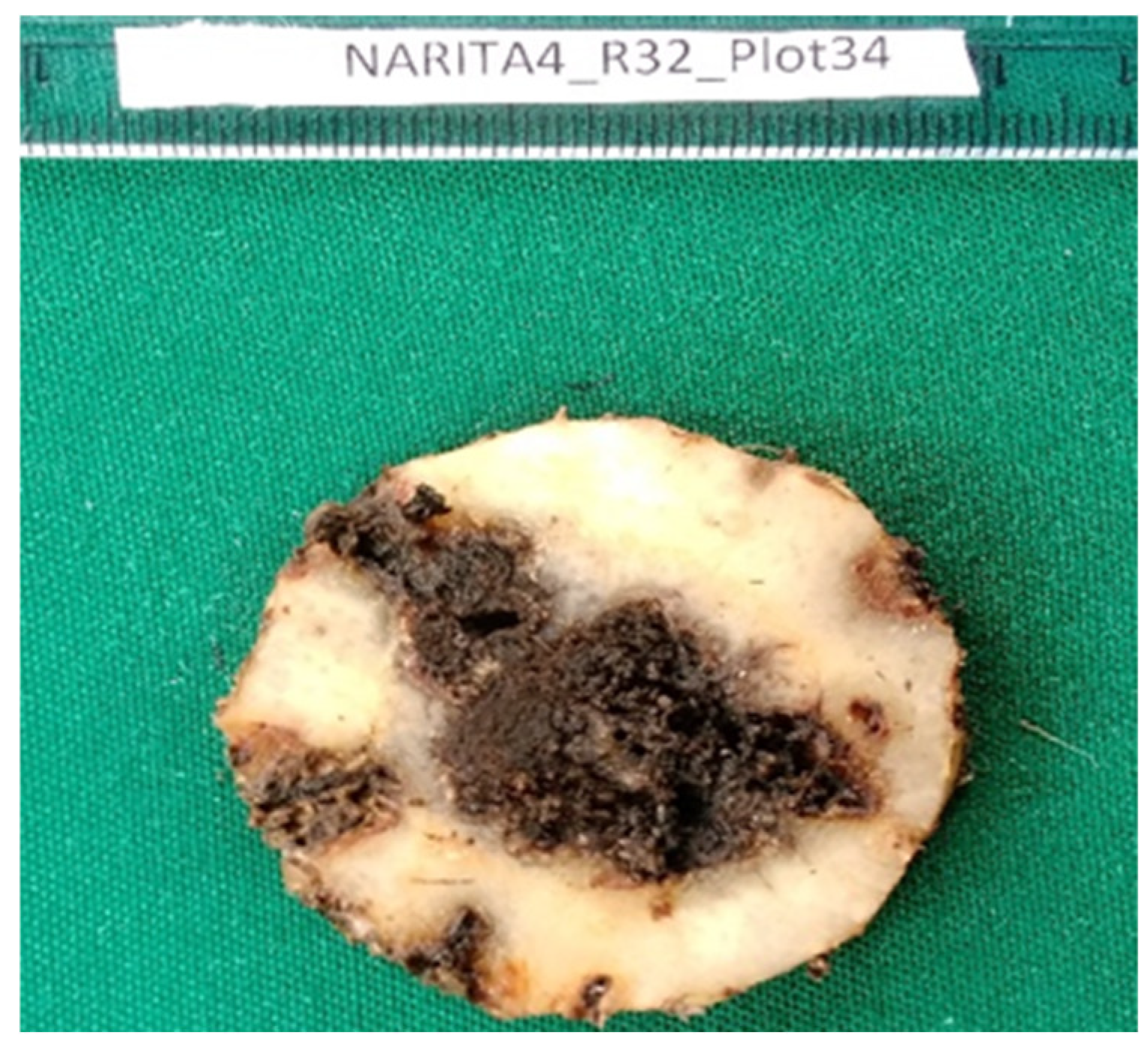
Figure 2.
(A)-Original image of banana corm as taken with the camera; (B)-Banana corm image processed using rembg script (0.3x magnification).
Figure 2.
(A)-Original image of banana corm as taken with the camera; (B)-Banana corm image processed using rembg script (0.3x magnification).
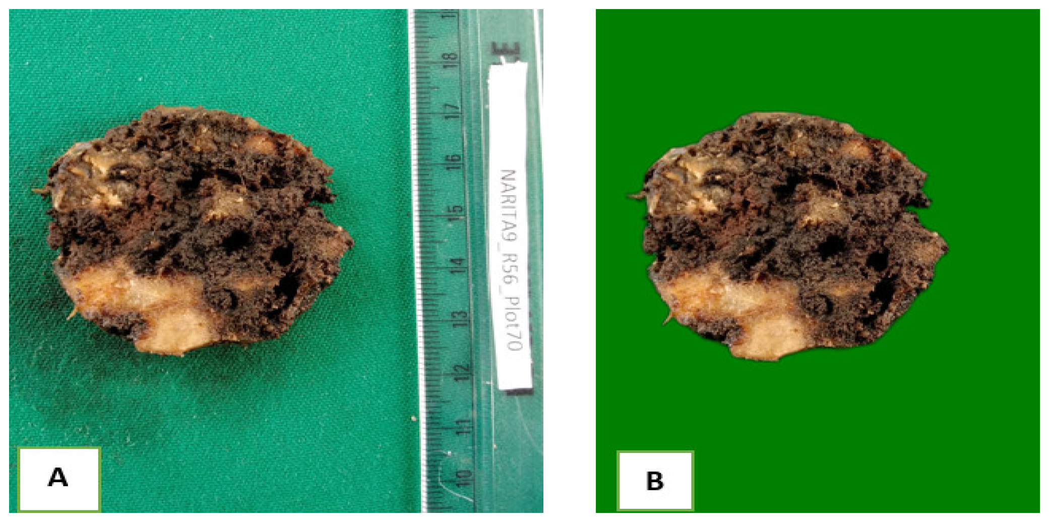
Figure 3.
Binary image generated by trained ilastik machine learning algorithm. Black is the weevil-damaged corm tissue and white the healthy corm tissue (0.4X magnification).
Figure 3.
Binary image generated by trained ilastik machine learning algorithm. Black is the weevil-damaged corm tissue and white the healthy corm tissue (0.4X magnification).
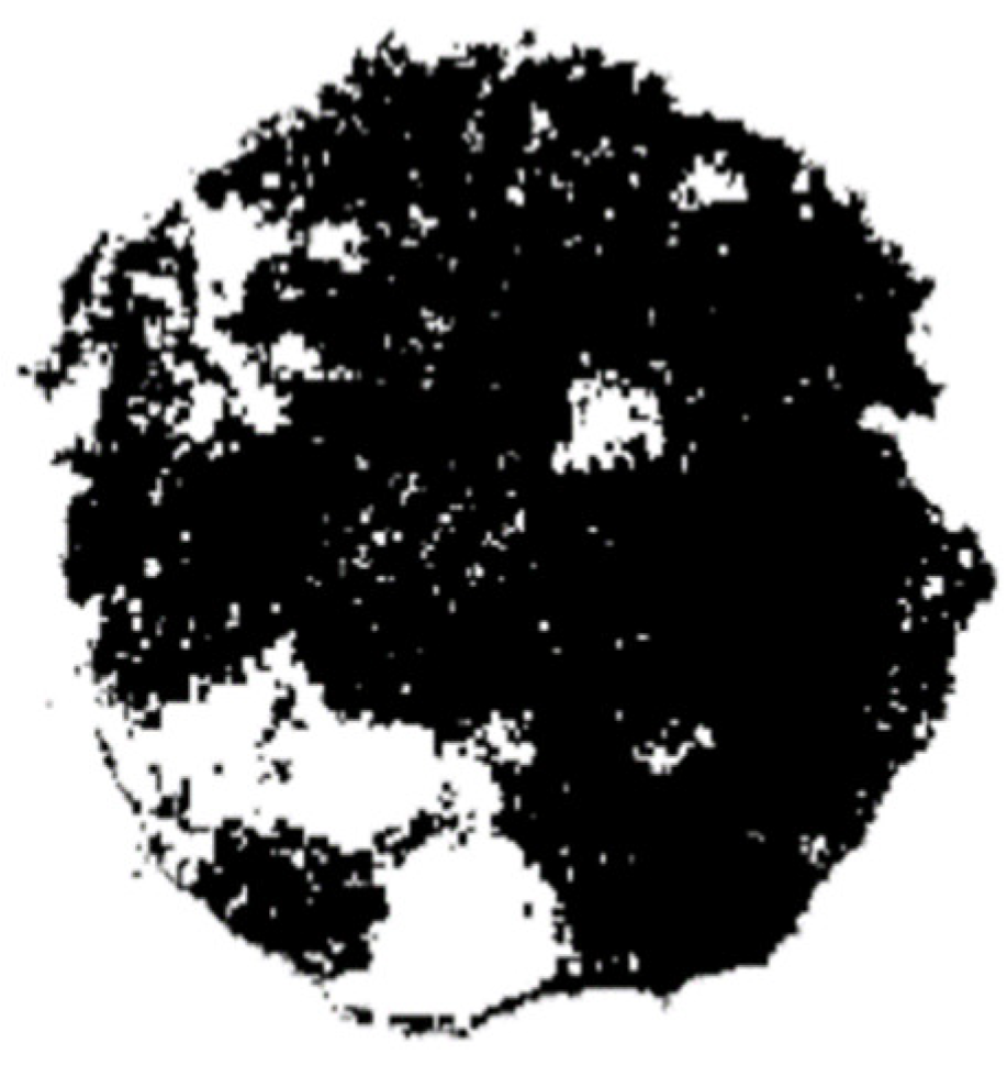
Figure 4.
Image annotation using the Makesense annotation tool.
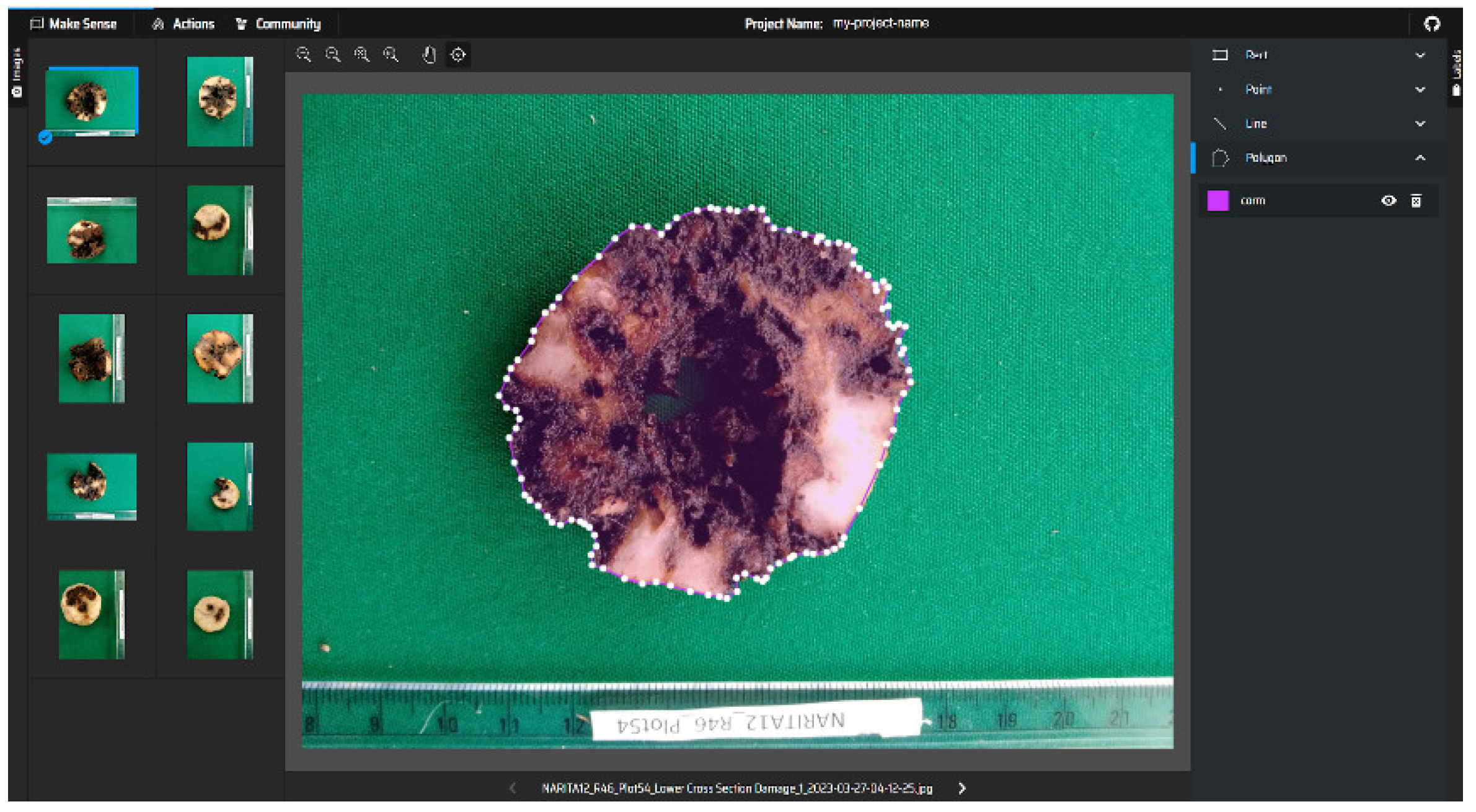
Figure 5.
An illustration of IOU: (A)- ground truth region with red boundary; (B)-predicted region with blue boundary; (C)-area of intersection between ground truth and predicted regions (shaded blue) – which is nearly 0.5 IOU since the area of overlap is almost half the ground truth and prediction region (0.2X magnification).
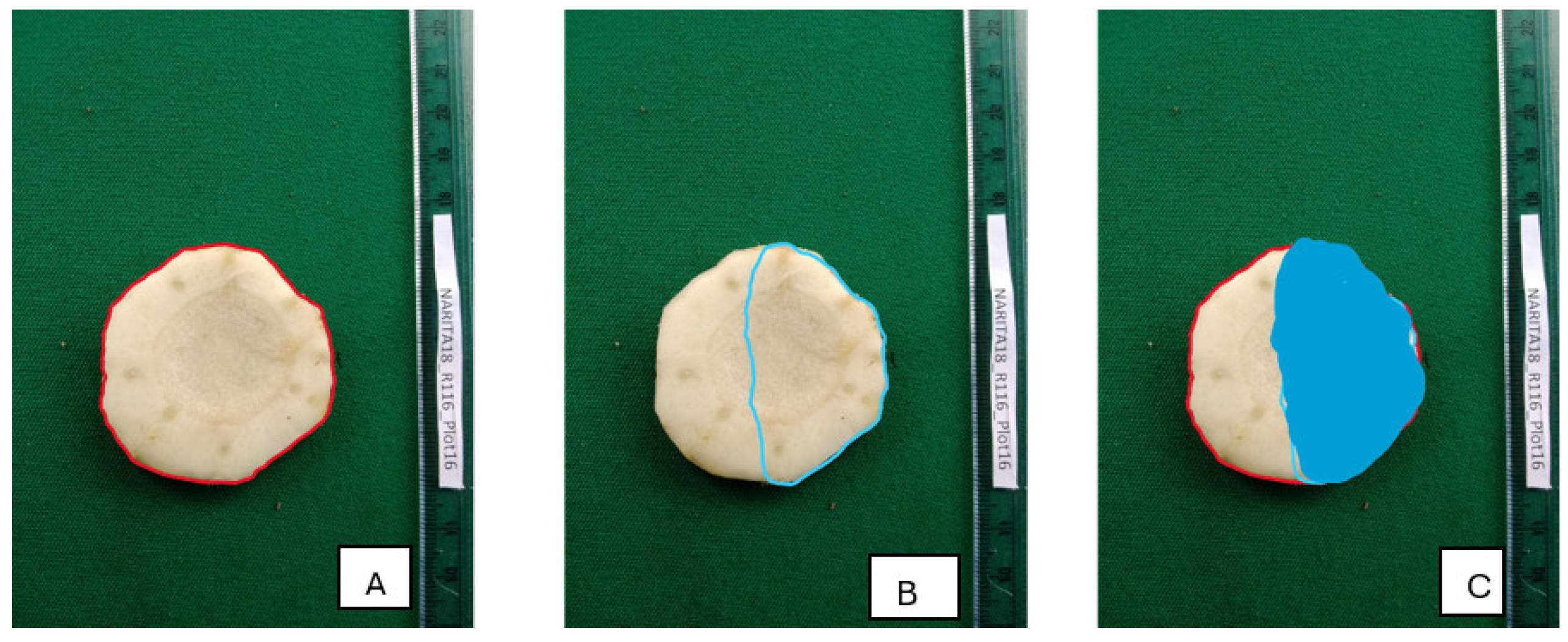
Figure 6.
Precision recall curve for the trained corm detection model with precision score on the y-axis and recall on the x-axis. The dashed green line represents the model’s performance for the ’banana’ class, with an average precision (AP) of 0.995. Similarly, the dashed red line represents the model’s performance across all classes (healthy and damaged tissue, and background), with a mean average precision (mAP) of 0.995 at an IoU threshold of 0.5. Banana is the name of the corm class used for the experiments.
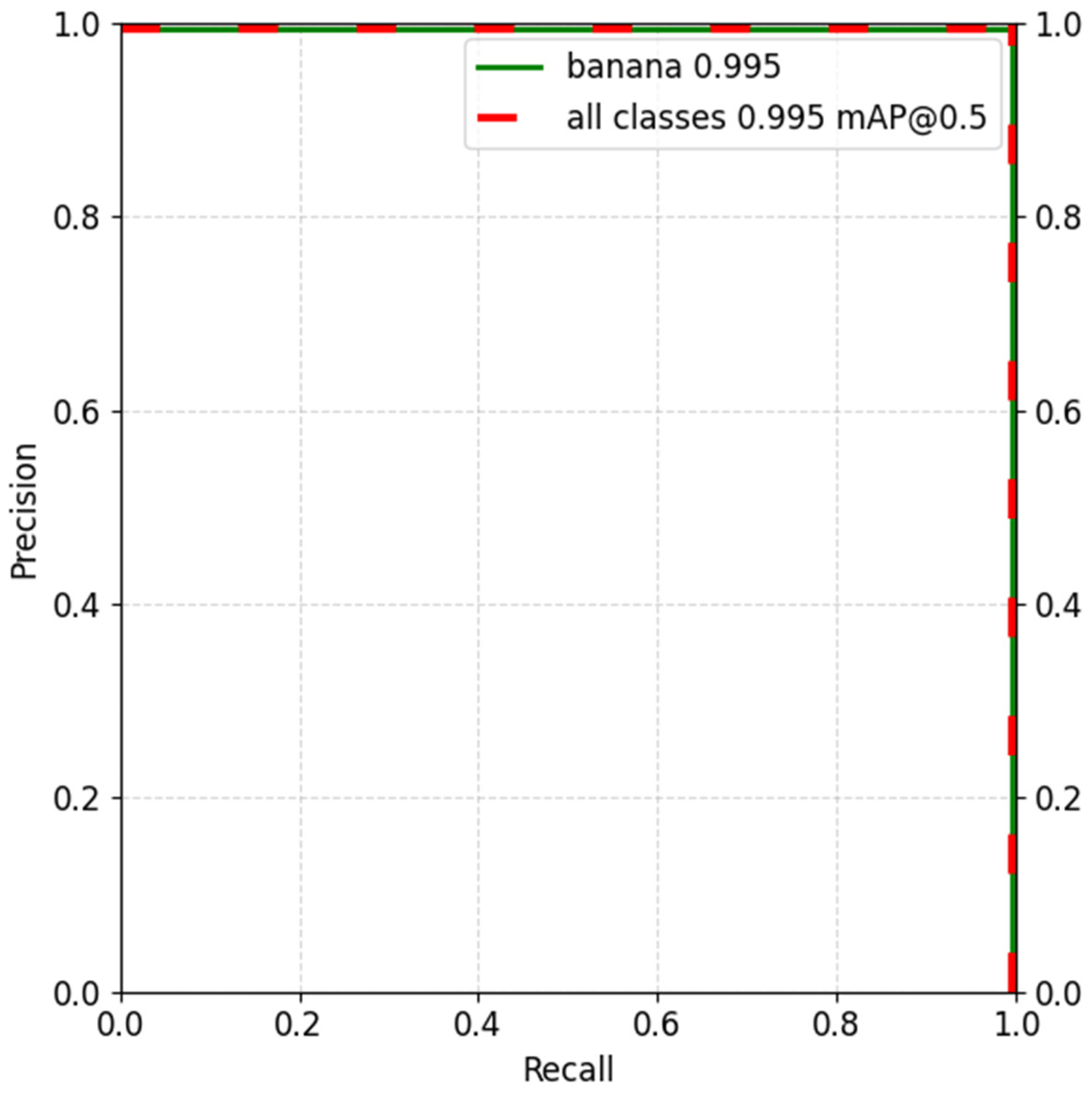
Figure 7.
A- original input image that is passed through the model; B- model predicted mask returned after analysis and C- result of background elimination (0.3x magnification).
Figure 7.
A- original input image that is passed through the model; B- model predicted mask returned after analysis and C- result of background elimination (0.3x magnification).
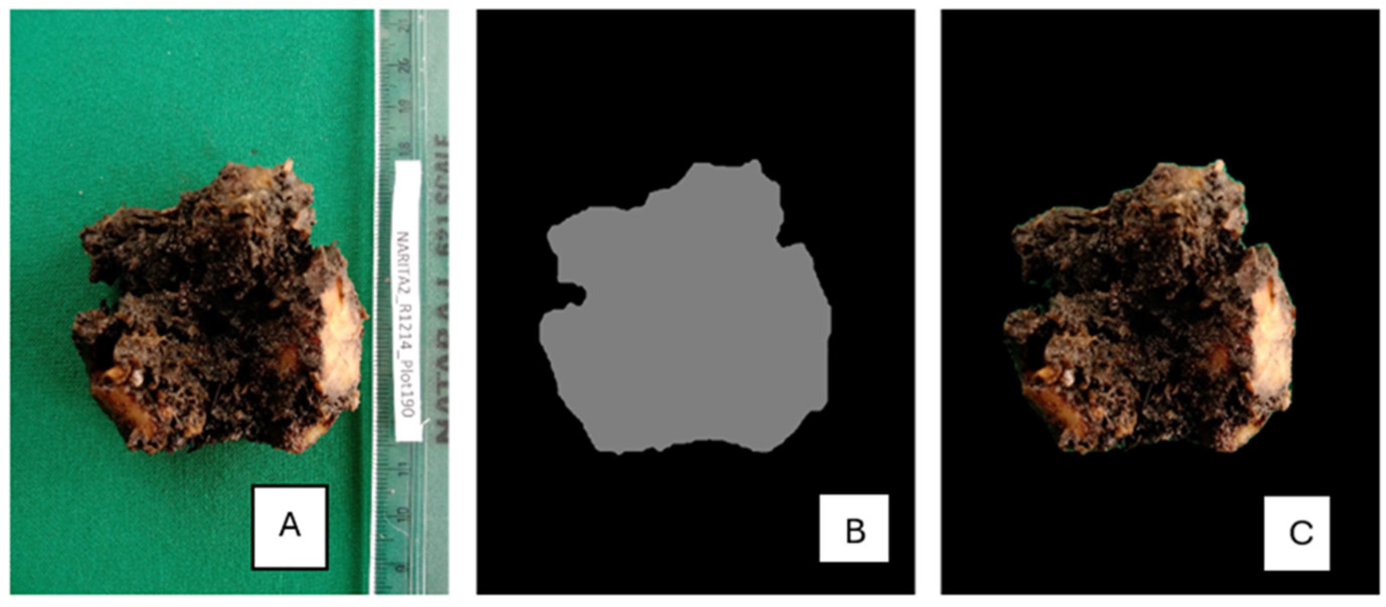
Figure 8.
a. Bland-Altman plot of mean differences between ImageJ and visual observation. (b). Bland-Altman plot of mean differences between machine learning and ImageJ. (c). Bland-Altman plot of mean differences between machine learning and visual observation.
Figure 8.
a. Bland-Altman plot of mean differences between ImageJ and visual observation. (b). Bland-Altman plot of mean differences between machine learning and ImageJ. (c). Bland-Altman plot of mean differences between machine learning and visual observation.
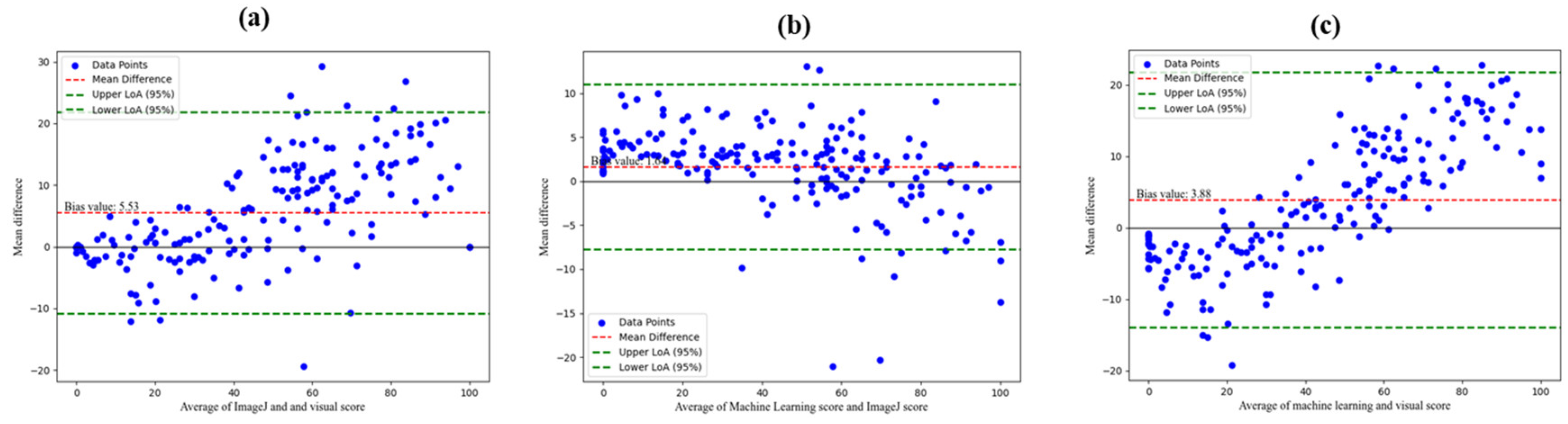
Figure 8.
a). Lin’s concordance correlation coefficient scatter plot between ImageJ and visual observation. (b) Lin’s concordance correlation coefficient scatter plot between machine learning and visual observation. (c) Lin’s concordance correlation coefficient scatter plot between ImageJ and machine learning.
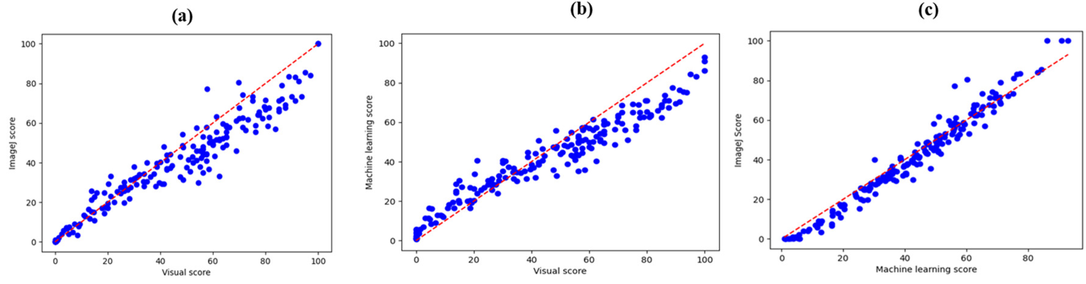
Figure 9.
Mean performance of genotypes for ImageJ, machine learning and visual observation for Calcutta 4 the resistant check, and landraces Mbwazirume, Mchare and Obino Lewai as the susceptible checks.
Figure 9.
Mean performance of genotypes for ImageJ, machine learning and visual observation for Calcutta 4 the resistant check, and landraces Mbwazirume, Mchare and Obino Lewai as the susceptible checks.
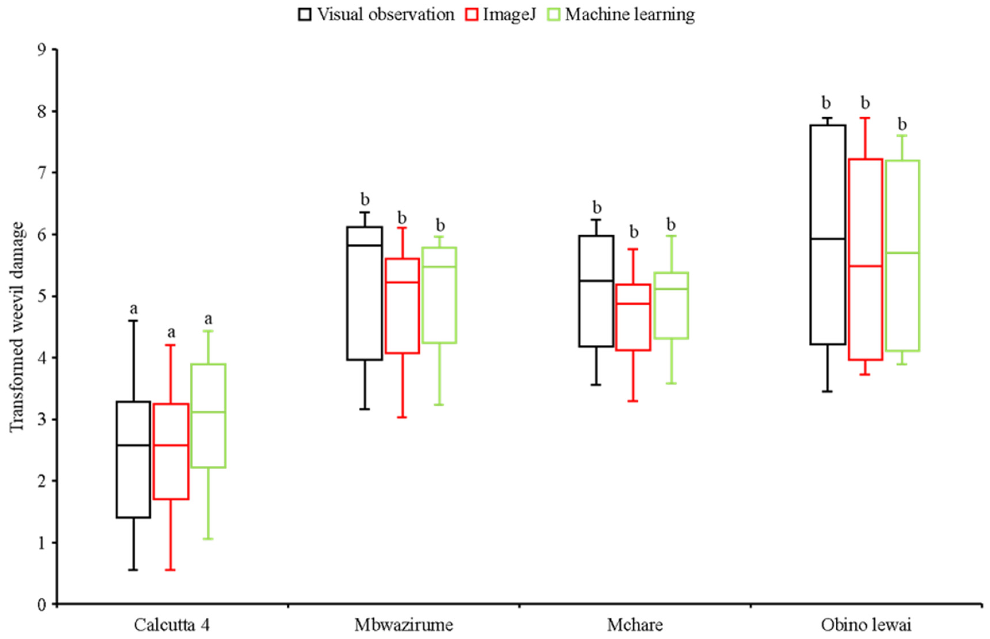

Table 1.
Interpretation of Lin’s CCC values.
| Value of the Lin’s CCC | Interpretation |
| >0.99 | Almost perfect |
| 0.95 to 0.99 | Substantial |
| 0.90 to 0.95 | Moderate |
| <0.9 | Poor |
Table 2.
Comparison of mean and standard deviation scores between the visual and ImageJ scoring.
| Score Method | Mean (%) | Standard deviation |
| Visual observation | 45.15 | 28.22 |
| ImageJ | 39.63 | 23.92 |
| Machine learning | 41.27 | 21.50 |
Table 3.
Concordance measures among weevil damage scoring methods.
| Score methods | Concordance Measures | |
| Pearson correlation coefficient (r) | Lin’s CCC | |
| ImageJ and visual observation | 0.96 | 0.89 |
| Machine learning and visual observation | 0.97 | 0.87 |
| ImageJ and machine learning | 0.98 | 0.96 |
Table 4.
Mean squares for each source of variation.
| Source of variation | Degrees of Freedom | Mean Square |
| Weevil scoring method | 2 | 3.668ns |
| Genotype | 21 | 24.306*** |
| Weevil scoring method*Genotype | 42 | 0.235ns |
| Residual | 489 | 2.605 |
ns = Not significant (p>0.05), *** = Significant different (p<0.001).
Disclaimer/Publisher’s Note: The statements, opinions and data contained in all publications are solely those of the individual author(s) and contributor(s) and not of MDPI and/or the editor(s). MDPI and/or the editor(s) disclaim responsibility for any injury to people or property resulting from any ideas, methods, instructions or products referred to in the content. |
© 2024 by the authors. Licensee MDPI, Basel, Switzerland. This article is an open access article distributed under the terms and conditions of the Creative Commons Attribution (CC BY) license (http://creativecommons.org/licenses/by/4.0/).
Copyright: This open access article is published under a Creative Commons CC BY 4.0 license, which permit the free download, distribution, and reuse, provided that the author and preprint are cited in any reuse.


