
Submitted:
23 December 2024
Posted:
24 December 2024
Read the latest preprint version here
Abstract
This paper investigates sustainability of additive manufacturing (AM) processes using machine learning (ML). Although AM is recognized as more sustainable than traditional manufacturing, the existing approaches to study AM sustainability are often time-consuming and resource intensive. This research fills the gap by directly linking AM parameters with sustainability metrics. Our research proposes a data-driven approach to predict sustainability outcomes and optimize AM processes. ML models of Linear Regression, Decision Trees, Random Forest and Gradient Boosting are evaluated to build a comprehensive framework which can understand AM process parameters and their effects on the AM sustainability. The findings demonstrate that ML can accurately predict AM sustainability based on relationships of AM parameters and their effects on sustainability. The optimal parameters can reduce the energy consumption and material waste in AM process. This work offers a scalable and efficient method to enhance AM sustainability. The results contribute to advancing sustainable AM practices and provide a foundation for the future exploration into broader AM processes.
Keywords:
Additive Manufacturing
; Sustainability
; Machine Learning
; Parameter Optimization
1. Introduction
Manufacturing is a cornerstone of industrial development and economic growth, playing a pivotal role in producing goods to meet societal demands [1]. However, traditional manufacturing methods often entail the significant resource consumption and waste generation, raising concerns about their environmental impact. The manufacturing sector accounts for a substantial share of global greenhouse gas emissions, energy consumption (15%), and material consumption (35-40%) [2]. Consequently, the quest for more sustainable manufacturing practices has become increasingly urgent in the face of climate change and resource depletion for a circular economy.
Additive Manufacturing (AM), commonly known as 3D Printing, has emerged as a revolutionary approach characterized by its layer-by-layer construction of parts from digital models. This innovative method contrasts sharply with conventional manufacturing (CM), which typically relies on subtractive processes to remove material from a larger block [3]. AM offers numerous advantages, including design flexibility, the ability to create complex geometries, and reduced material waste. AM can minimize the waste and optimize resource utilization. Furthermore, AM enables the production of products close to end users, reducing transportation emissions and enhancing supply chain efficiency [4].
The AM sustainability potential can be further amplified by its capability to fabricate lightweight structures that meet stringent performance requirements, making it particularly attractive for industries such as aerospace, automotive, and healthcare, where material efficiency and performance are paramount [5]. Additionally, AM facilitates the use of alternative and recycled materials, contributing to a more sustainable lifecycle for products [6]. However, despite its inherent advantages, the widespread adoption of AM faces challenges such as variability in material properties, process parameters, and complexities of optimizing designs.
In this context, AM sustainability encompasses not only environmental considerations but also social and economic dimensions. It refers to meeting current production needs while ensuring that future generations can fulfill theirs without depleting resources or harming the environment [7]. To fully embrace sustainable practices in AM, it is essential to quantify and analyze various operational parameters for their impact on sustainability metrics. Machine learning (ML) has emerged as a promising approach to address this need, offering powerful tools for analyzing complex datasets and uncovering relationships between parameters and performance outcomes.
Integrating ML into the AM framework enables researchers to predict mechanical properties and assess their direct impact on sustainability metrics, such as energy consumption, material efficiency, and overall environmental impact [8]. By employing advanced algorithms, ML can analyze vast amounts of data generated during the AM process [9], facilitating the optimization of parameters like layer thickness, infill type, and build orientation. This data-driven approach not only enhances the process efficiency but also supports informed decision-making regarding sustainability. The contribution of this research is its direct focus on sustainability outcomes, integrating both environmental and economic dimensions to demonstrate specific parameter choices for overall sustainability. By employing ML, it can predict outcomes and uncover relationships between parameters and sustainability metrics, showing importance of the parameter optimization in achieving efficient and sustainable AM processes. This innovative approach provides a scalable solution for advancing AM sustainability, addressing a gap in current research and offering valuable insights for the future developments.
2. Literature Review
AM builds parts layer by layer, guided by digital models, which significantly reduces the material waste and energy consumption compared to CM [3]. Due to these advantages, AM is often considered a more sustainable option than CM [7].
Sustainability of manufacturing processes including AM is commonly assessed by three primary approaches: cradle-to-grave [10], cradle-to-gate [11], and gate-to-gate [12]. The cradle-to-grave approach evaluates sustainability metrics like energy consumption and material usage from raw material extraction to product's disposal after its useful life. Cradle-to-gate focuses on these metrics from the raw material extraction to production stage, while gate-to-gate examines only the production process. Analysis methods employed in these approaches include Life Cycle Costing (LCC) which focuses on the total economic cost, and Life Cycle Assessment (LCA) which evaluates environmental impacts over the product's lifecycle [13].
Various approaches have been proposed to investigate AM sustainability. Some studies have focused on energy consumption and material usage as key indicators of AM sustainability [14]. Energy consumption in AM encompasses multiple stages, including the warm-up time, printing time, post-processing, and material processing, all of them contribute to the overall energy demand. Additionally, factors such as machine's efficiency and its rate of utilization play a crucial role in determining energy use. A machine running at the optimal capacity with high utilization rates tends to be more energy-efficient, as downtime and idle energy consumption are minimized. In contrast, a low utilization or inefficient operation can lead to wasted energy [15]. Moreover, the quantity and type of material processed, whether metals, polymers or composites, can influence the energy required for both material handling and post-processing stages. Insightfully managing these aspects is a key to enhancing AM sustainability by optimizing the energy use while maintaining production quality [16]. Others have examined relationships between electrical energy consumption and emissions to assess AM sustainability [17]. In the context of metal AM, energy [18] and exergy [19] metrics have been used to evaluate sustainability. Additionally, some studies have explored the recyclability of PET filaments to assess sustainability for the material usage [20]. Design plays a pivotal role in achieving AM sustainability. By leveraging the AM flexibility, designers can optimize part geometries to reduce material usage, create lightweight structures, and minimize waste. Features such as topology optimization and lattice structures allow for efficient designs that maintain strength while using less material [21]. Furthermore, design for recyclability and modular components can extend product life cycles, facilitate remanufacturing, and enhance material recovery, contributing to a circular economy. Thoughtful design choices in AM can not only improve resource efficiency but also reduce energy consumption in the manufacturing process [22]. Although these studies have made significant contributions to understanding AM sustainability, approaches they used are often time-consuming, labor-intensive, and resource-intensive, requiring extensive experiments and data collection to draw meaningful conclusions.
To address the challenges of AM sustainability, ML tools have been increasingly studied for their potential to predict and optimize various processes [23]. By focusing on key mechanical properties such as tensile strength, compressive strength, and Young’s modulus, researchers have harnessed ML techniques to enhance the efficiency of AM. While specific models like Regression [24], Classification [25], and Neural Networks (NN) [26, 27] have been employed, the overarching goal remains the same: optimizing AM processes to reduce waste and energy consumption. For instance, the prediction of tensile strength through ML allows for the identification of optimal processing parameters, which improves the part quality and minimizes defects [28, 29]. It is crucial as defects in printed parts often lead to increased material waste and longer production times. Similarly, by accurately predicting the compressive strength [30] and Young's modulus [31], ML can facilitate the design of components to meet performance specifications without the excess material usage. Moreover, the integration of ML into parameter optimization strategies [32, 33], such as adjusting layer thickness, infill type and build orientation, contributes significantly to sustainability efforts [14]. These efforts can reduce the need for trial-and-error methods traditionally used in AM, thereby decreasing production time and energy consumption.
Despite advancements in utilizing ML for predicting mechanical properties, a significant gap remains in directly correlating AM parameters with sustainability metrics. While the indirect benefits of enhancing mechanical properties and reducing defects are evident, further research is essential to establish clear connections between specific ML applications and sustainability outcomes in AM. Understanding how specific AM parameters impact sustainability metrics is crucial for improving the overall efficiency and environmental performance of the AM process. This research aims to directly analyze this relationship by evaluating different ML models and present optimized parameters offering a substantial advancement over traditional time-consuming, and resource-intensive approaches to studying sustainability. By integrating sustainability assessments into the ML modeling framework, our research introduces a novel data-driven method that examines key parameters such as layer thickness, number of shells, build orientation, infill type, and infill percentage. Impacts of these parameters are evaluated on energy consumed, weight of the part, scrap-weight, and printing time, a comprehensive framework is introduced for AM sustainability. Bridging this gap could ultimately lead to the development of sustainable AM practices that align with industry goals and environmental standards, fostering more informed decision-making in the field.
3. Methodology
In this section, we will discuss the ML models evaluated, hyperparameter optimization, evaluation metrics, data collection, and sustainability metrics.
3.1. ML Models
3.1.1. Linear Regression (LinReg)
Linear regression is a technique used in statistics and machine learning to model the relationship between dependent and independent variables, assuming a linear relationship. Changes in the dependent variable occur proportionally with changes in the independent variables, as shown in the equation below:
where Y is the dependent variable, X is the independent variable, is the intercept, is the slope of the line, and ε represents the error between the predicted and actual values [31].
By minimizing the sum of squared differences between the true and predicted values, linear regression identifies the best-fit line, a process known as the least squares method. It is most effective for linear data with the minimal noise.
3.1.2. Decision Tree (DT)
Decision Trees are simple yet powerful regression models that split the data recursively into regions with minimal target variance. They are particularly intuitive, as they create a flowchart-like structure where each internal node represents a decision rule, and leaf nodes correspond to predictions. However, DTs are prone to overfitting due to their tendency to memorize training data [26].
Mathematically, the decision at each split minimizes the Mean Squared Error (MSE):
where is the actual value, is the mean of the target values in a region, n is the number of data points in the region.
The tree grows until a stopping criterion, such as the maximum depth or minimum samples per leaf, is met. Predictions are made by taking the mean of target values in the corresponding region.
3.1.3. Random Forest (RF)
Random Forest enhances the performance of Decision Trees by using an ensemble of trees trained on bootstrapped subsets of the data. Each tree randomly selects a subset of features for splitting, introducing randomness that reduces overfitting and improves generalization. RF is robust to noise and highly effective in predicting complex patterns [28].
For regression, RF predicts by averaging the outputs of all the T trees:
where is the prediction of the t-th tree.
By combining the strengths of multiple weak learners, RF provides accurate and stable predictions while remaining resistant to overfitting.
3.1.4. Gradient Boosting (GB)
Gradient Boosting is an advanced ensemble technique that builds trees sequentially, where each tree corrects the residuals of the previous trees. Unlike RF, which trains trees independently, GB uses a gradient descent approach to optimize a loss function, typically the MSE for regression tasks. This iterative refinement allows GB to capture complex relationships effectively [34].
The residuals at iteration t are computed as:
where is the actual value, and is the prediction from the previous iteration.
The updated prediction is:
where η is the learning rate, and is the prediction from the t-th tree.
GB's iterative error minimization makes it highly accurate, but it requires careful tuning of hyperparameters to prevent overfitting or underfitting.
3.2. Hyperparameter Optimization
For parameter optimization and response variable predictions, the model initializes by importing necessary libraries and defining a dataset with various parameters related to AM. It employs ML models such as the DT and RF regressors to predict multiple response variables like the energy consumed, weight of the part, scrap weight and printing time. Both models utilize a ‘random_state’ parameter to ensure reproducibility of results. The RF model also includes an ‘n_estimators’ parameter, setting the number of trees in the forest to 100. The data is split into training and test sets with 20% of the data reserved for testing, using a random state to keep splits consistent across different runs [34]. The ‘StandardScaler’ is applied to normalize feature scales, enhancing model performance. Additionally, the minimize function from the ‘scipy.optimize’ library is used to find optimal parameters for minimizing response variables, utilizing the ‘L-BFGS-B method’. This comprehensive setup aims to fine-tune the models and optimize the manufacturing parameters to minimize costs and improve efficiency. Table 1 highlights the hyperparameters configuration for the two models used for parameter optimization.
3.3. Evaluation Metrics
The models’ performance is assessed using the Coefficient of Determination (R²), Mean Absolute Error (MAE) and Mean Squared Error (MSE) [30].
R², MAE, and MSE are fundamental metrics used to evaluate the accuracy of regression models. R², or the coefficient of determination, quantifies the percentage of the variance in the dependent variable that is predictable from the independent variables, with values closer to 1 indicating a better fit of the model [26], mathematically represented as:
where (Sum of Squares of Residuals) = , (Total sum of squares) = , = actual values, =predicted values, and = mean of actual values.
Mean Absolute Error (MAE) measures the average magnitude of errors in predictions, giving a straightforward indication of prediction accuracy with a perfect score of 0, mathematically represented as:
where is the absolute error between the actual and predicted values.
Meanwhile, Mean Squared Error (MSE) calculates the average of the squares of the errors, heavily penalizing larger errors, which makes it sensitive to outliers in the data set, mathematically represented as:
These metrics together provide a comprehensive overview of a model’s predictive performance, helping in both the diagnostics of model behavior and the comparison of different models under consideration [35].
3.4. Data Collection and Preprocessing
To evaluate the AM sustainability, four key metrics including energy consumption, part weight, scrap weight, and printing time are used. The investigation employs five parameters at three levels to utilize the Taguchi Orthogonal Arrays approach as detailed in Table 2 [14].
Figure 1 displays the different parameter combinations used in the study for 3D Printing specimens. Categorical variables such as infill type and build orientation are converted into numeric values using the Python library ‘pd.Categorical’ for enhanced visualization. For example, infill types—cross-infill, diamond, and honeycomb—are initially encoded as 0, 1, and 2 respectively. Similarly, build orientations—flat, on-edge, and upright—are assigned values of 0, 1, and 2. For ML training and testing, these categories are further encoded as cross 1, diamond 2, honeycomb 3, flat 1, on edge 2, and upright 3, ensuring clear and effective data representation and model input standardization.
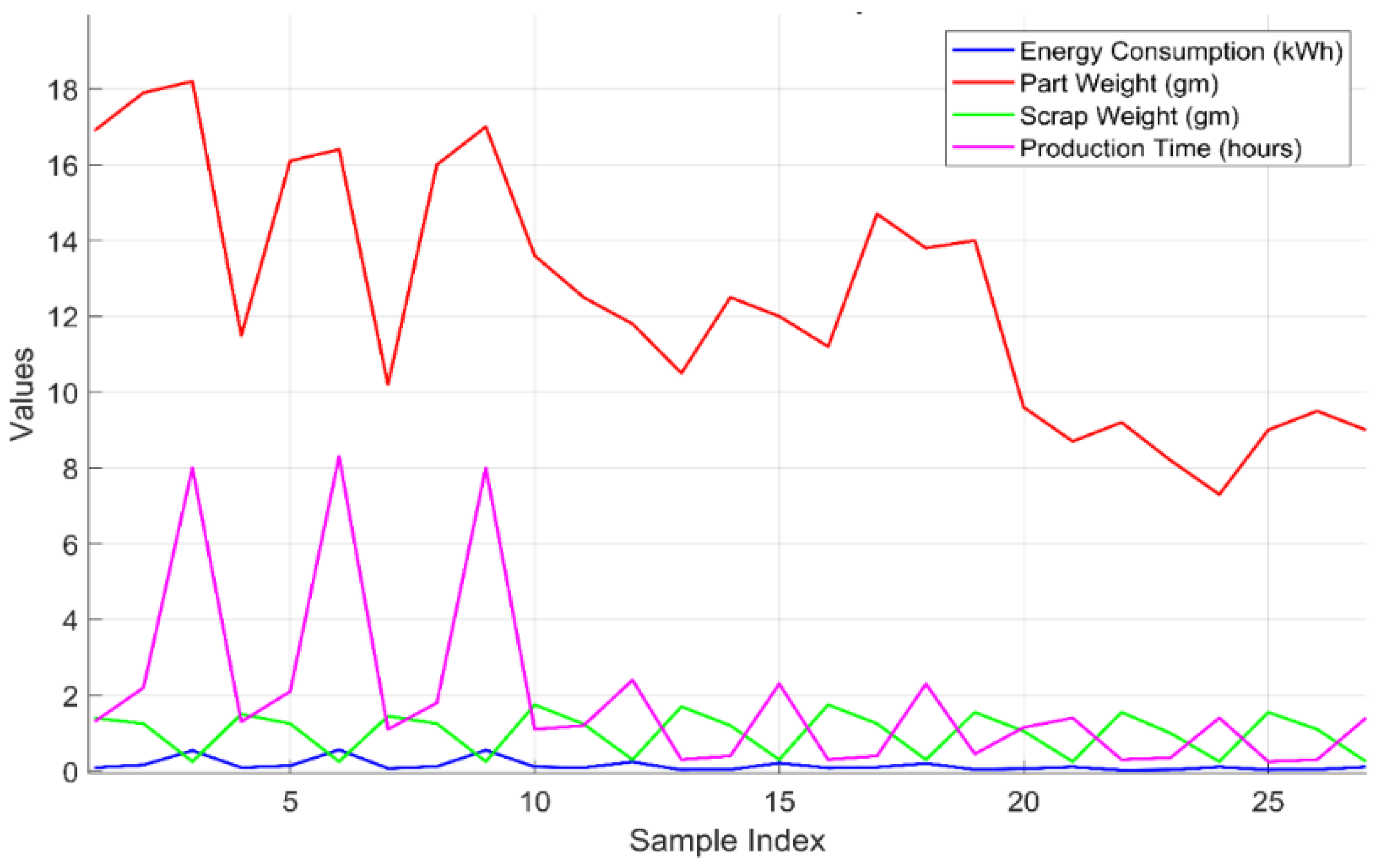
Figure 2 shows dimensions of the experimental specimen. Figure 3 displays 3 building orientations. Figure 4 presents the experimental data collected for the four-sustainability metrics. The x-axis represents the sample index, while the y-axis displays the corresponding values for each metric, allowing for a clear comparison across the different samples in terms of energy consumption, part weight, scrap weight, and production time. The energy consumed is determined by multiplying the 3D printer's power consumption by the sum of the warm-up and printing times. Part weight and scrap weight are measured by weighing the printed part and any additional materials such as support structures, respectively. Production time encompasses both set-up and printing durations.
Figure 1.
Parameter combinations for experiments.
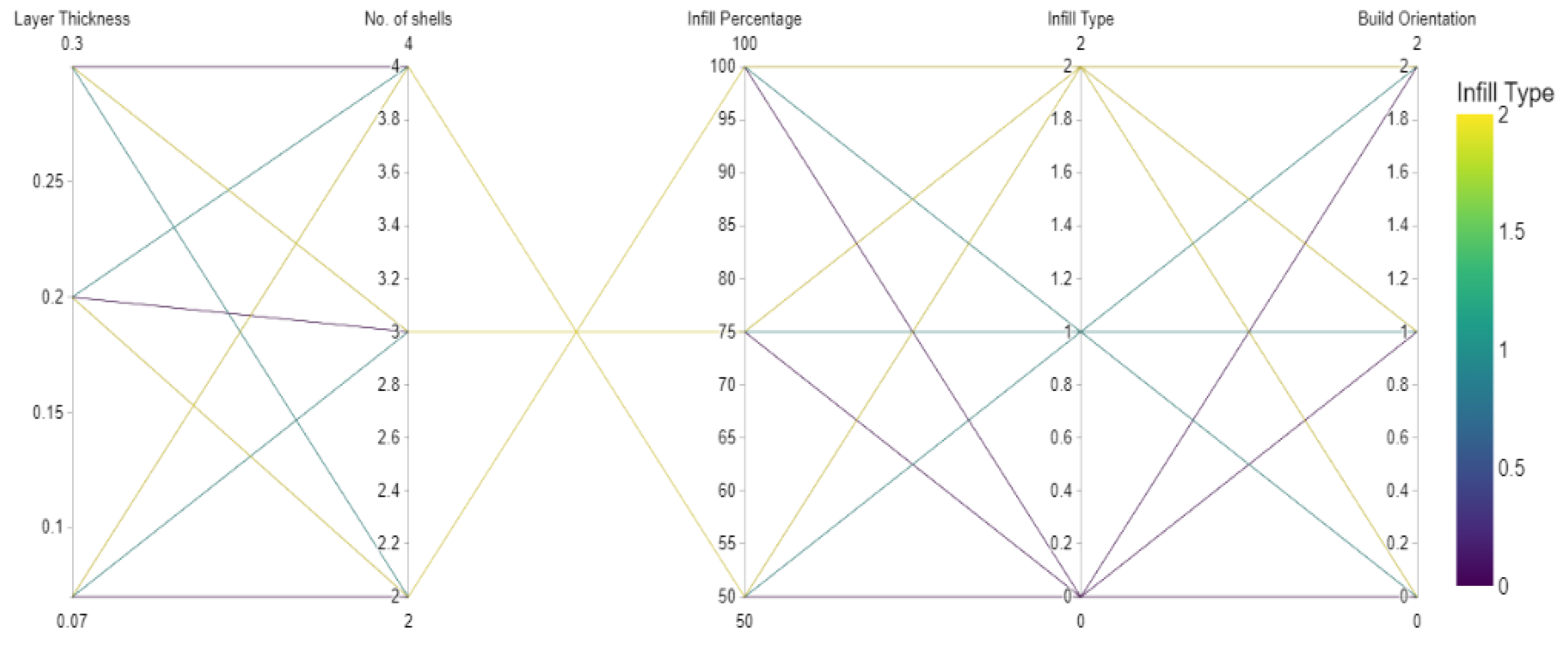
Figure 2.
Experimental specimen [14].
Figure 2.
Experimental specimen [14].
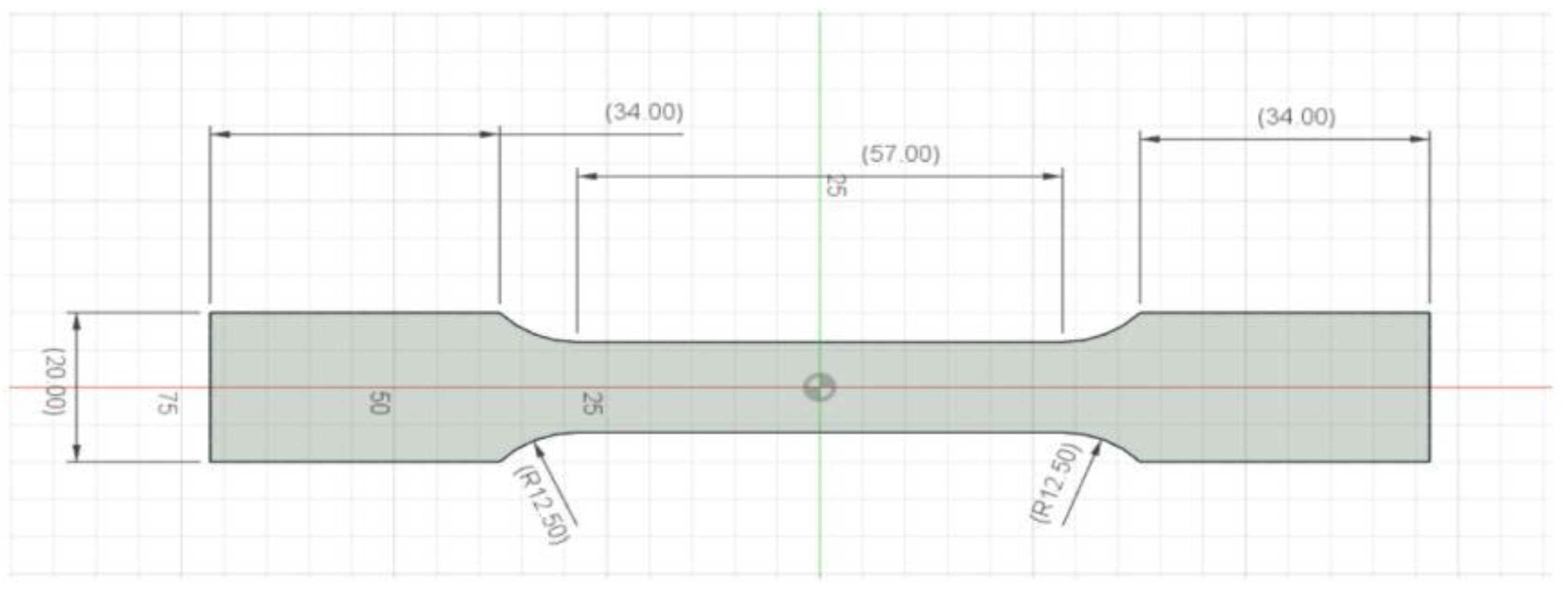
Figure 3.
Building orientations: (a) Flat; (b) On-edge; (c) Up right [14].
Figure 3.
Building orientations: (a) Flat; (b) On-edge; (c) Up right [14].
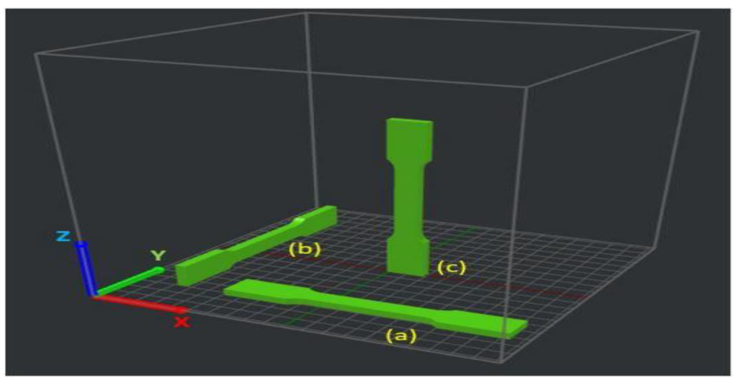
Figure 4.
Experimental data for: (a) Energy consumption; (b) Part weight; (c) Scrap weight; (d) Production time.
Figure 4.
Experimental data for: (a) Energy consumption; (b) Part weight; (c) Scrap weight; (d) Production time.
3.5. Sustainability Metrics
Among three aspects of sustainability, i.e. economic, environmental and social sustainability [36], this research focuses on the economic and environmental aspects of sustainability. Energy efficiency, material efficiency, and process efficiency are key factors that contribute to both environmental and economic sustainability [2,37]. Energy efficiency reduces energy consumption to lower operational costs and minimizes the carbon footprint. Material efficiency involves optimizing the resource use and reducing waste, which helps conserve natural resources and decrease pollution [15]. Economically, it leads to cost savings by reducing input materials. Process efficiency enhances production rate to lower energy use and reduce costs, improving both profitability and environmental impact.
. In AM, sustainability metrics such as energy consumption, part weight, scrap weight, and production time can be quantitatively represented to evaluate the environmental impact and efficiency of the printing process. The mathematical representation of each of these metrics is given below.
3.5.1. Energy Consumption (EC)
It can be represented as the total kilowatt-hours (kWh) used during the production of a single part and the warm-up time [10].
where is the power rating of the 3D printer (in kilowatts), is the time the printer takes to warm-up, and is time taken to print the part (in hours).
3.5.2. Part Weight (PW)
The total mass of the final product, usually measured in grams or kilograms [38] is represented as:
where is the mass of each component of the part if the part consists of multiple components.
3.5.3. Scrap Weight (SW)
The total mass of waste material generated during the printing process [38] is represented as:
where is the weight of the waste material for each print job.
3.5.4. Production Time (PT)
The total time required to produce a part, which includes setup time, printing time, and post-processing time [38] is represented as:
where is the time for setting up the printer, is the actual printing time, and
is the time required for any post-processing steps.
4. Results and Discussion
This section presents results and discussions of the ML models performance and the relationship analysis of parameters to the response variables.
4.1. ML Models Evaluation
We evaluate the performance and stability of four ML models, LinReg, DT, RF, and GB, in predicting the sustainability metrics of energy consumed, material used, scrap weight, and printing time in AM. The performance metric plots (e.g., R² and MSE) and model stability plots are applied in a comprehensive evaluation.
4.1.1. Performance Evaluation
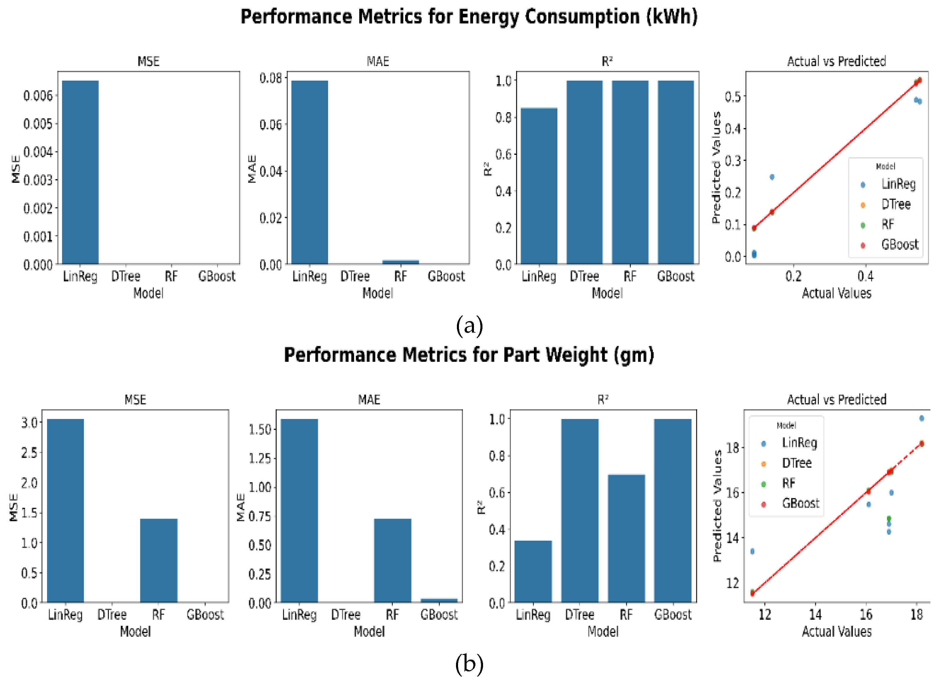
The performance metric plots in Figure 5 clearly highlight the superiority of the RF model across all response variables. In Figure 5a for MSE and MAE, RF consistently achieves the lowest values, indicating its ability to minimize prediction errors effectively. Similarly, in Figure 5c, RF secures the highest R² values, nearing 1, signifying exceptional alignment between predicted and actual values. This performance underscores RF's robustness and accuracy, which stems from its ensemble structure that combines predictions from multiple decision trees. DT, shown alongside RF in Figure 5a,c for part weight and scrap weight respectively, achieves competitive R² values and low MSE and MAE, making it a strong secondary choice despite slightly lower precision.
Figure 5b,c further demonstrate the limitations of LinReg and GB. LinReg, as evident in its high MSE in Figure 5a and lower R² values in Figure 5c, struggles with the non-linear relationships present in the dataset. GB performs moderately but is less consistent than RF and DT, with higher variability as seen in Figure 5a.
The "Actual vs. Predicted" performance is highlighted in all parts of Figure 5. Across each metric (energy consumption, printing time, material used for part weight, and scrap weight), RF's predictions align almost perfectly with the red diagonal line, reflecting its strong predictive performance across all metrics. In Figure 5a–d, DT also demonstrates good alignment between predicted and actual values, although with slightly more deviation compared to RF. LinReg, as seen in Figure 5a–d, shows significant deviations, particularly in regions of higher complexity, where scattered points fall far from the red line. GB exhibits moderate alignment across the same figures but suffers from occasional outliers, highlighting sensitivity to parameter tuning. These "Actual vs. Predicted" trends reinforce RF's dominance and DT's reliability, while LinReg and GB underperform consistently across all metrics.
Figure 5.
Performance metrics of the ML models for: (a) Energy Consumption; (b) Part Weight; (c) Scrap Weight; (d) Production Time.
Figure 5.
Performance metrics of the ML models for: (a) Energy Consumption; (b) Part Weight; (c) Scrap Weight; (d) Production Time.
4.1.2. Model Stability Analysis
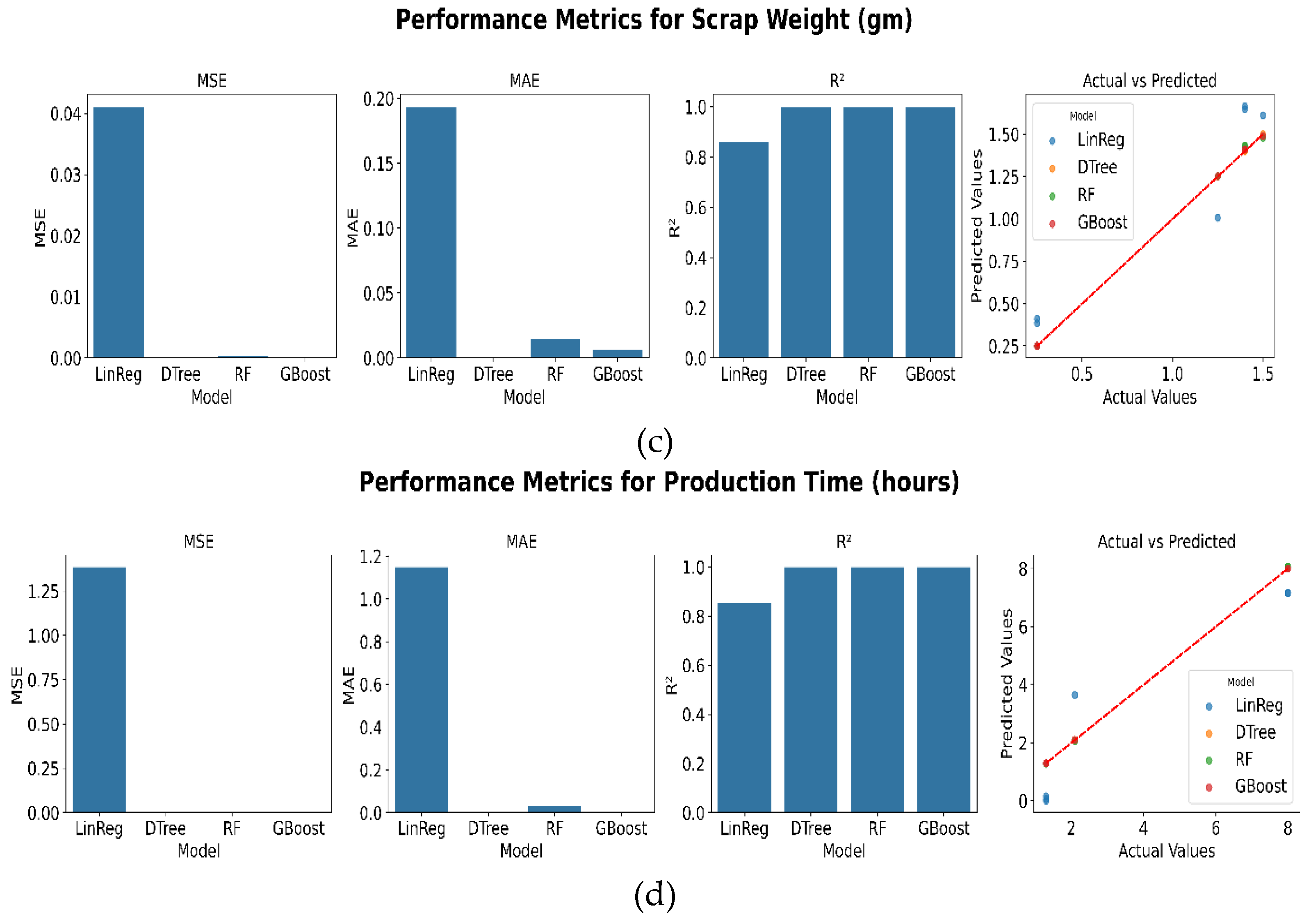
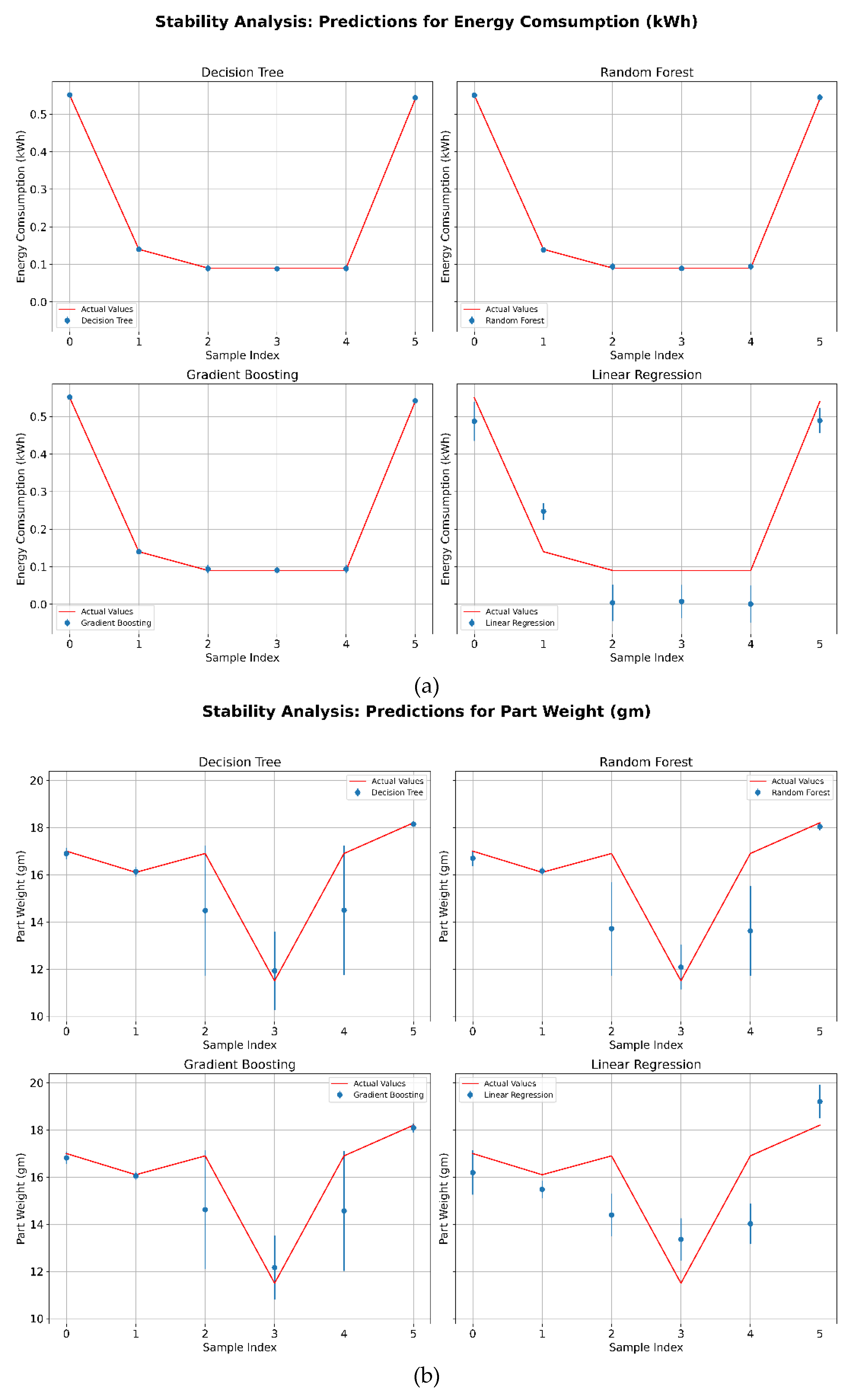
The stability plots in Figure 6 provide a detailed visualization of the consistency of predictions for different models across various parameter combinations, helping us draw key conclusions about their performance. For RF, the narrow confidence intervals displayed in the plots in Figure 6a–d demonstrate its minimal prediction variability, as seen by the blue points closely aligning with the red lines (actual values). This consistent alignment across all parameter combinations highlights RF's robustness and reliability, making it particularly well-suited for applications in AM, where prediction stability is critical. The lack of large deviations in RF's plots indicates its ability to generalize effectively, regardless of the parameter complexity.
In comparison, the DT model also shows relatively consistent predictions in its plot, with blue points closely following the red lines. However, the confidence intervals for DT are slightly wider than those of RF, particularly in regions where parameters are more variable, such as in Figure 6a,d. This indicates moderate variability in DT's predictions, suggesting that while it remains reliable, it is not as robust as RF for scenarios requiring high precision.
The LinReg model, on the other hand, exhibits significant instability in its predictions, as evident from the wide confidence intervals and inconsistent alignment of blue points with the red lines. For instance, in nonlinear regions such as in Figure 6a,d, LinReg fails to follow the trend of actual values, leading to erratic predictions. These deviations in the plot indicate that LinReg struggles to handle nonlinear interactions, making it unsuitable for complex AM parameter optimization tasks.
GB demonstrates moderate stability in its predictions, as observed in its plot where the blue points align reasonably well with the red lines in Figure 6a,d, energy consumption and printing time respectively. However, occasional spikes in variability can be seen, such as around in Figure 6b,c for part weight and scrap weight respectively, where confidence intervals widen significantly. These spikes suggest that GB is sensitive to certain parameter changes, which can limit its effectiveness in scenarios requiring highly consistent predictions.
By examining plots in Figure 6, findings can be related to the observed trends and prediction patterns. For instance, RF's narrow confidence intervals and tight clustering of blue points around the red lines clearly showcase its stability and reliability. In contrast, LinReg’s wide intervals and scattered blue points highlight its instability, while GB’s occasional deviations and moderate alignment reflect its sensitivity to parameter changes. The DT plot shows stable predictions overall, with slightly more variability than RF but far better alignment than LinReg. These visual patterns directly support the conclusion that RF is the most robust and reliable model for AM applications, with DT as a secondary choice, while LinReg and GB exhibit limitations in handling complex parameter spaces.
Figure 6.
The ML models Prediction Stability Analysis for: (a) Energy Consumption; (b) Part Weight; (c) Scrap Weight; (d) Production Time.
Figure 6.
The ML models Prediction Stability Analysis for: (a) Energy Consumption; (b) Part Weight; (c) Scrap Weight; (d) Production Time.
4.1.3. Model Selection and Parameter Optimization
The selection of RF and DT ML models for detailed evaluation is based on a balance between performance and stability. RF, with its superior accuracy and low variability, is ideal for precise and consistent predictions. DT, while less accurate, offers stability and interpretability, making it a valuable complementary model. LinReg and GB, due to their higher variability and weaker performance metrics, are less suitable for this application.
Figure 7 illustrates the high performance of the DT and RF models on the test set, as evidenced by consistently high R² scores across all response variables. RF demonstrates superior generalization with test set R² scores close to 1, indicating exceptional accuracy in capturing the underlying patterns of energy consumption, production time, part weight, and scrap weight. DT also performs well, though with slightly lower R² scores compared to RF, reflecting minor variability in prediction accuracy. This strong alignment between predicted and observed values highlights the robustness of both models, particularly RF, in parameter optimization and predictive reliability.
Table 3 lists the optimized parameters derived from the models, highlighting key combinations of AM parameters that contribute to minimizing energy consumption, reducing production time, and ensuring consistent part weight and scrap weight. These results demonstrate the practical utility of ML models in guiding AM practices.
4.2. Relationship Analysis between Process Parameters and Response Variables
The correlation analysis is presented in Figure 8 using both bar plots (left) of correlation coefficients and heatmaps (right) of pairwise correlations, which provides a comprehensive understanding of the relationships between features and response variables [39]. The bar plots Figure 8(left) highlight building orientation as the most influential feature across all response variables, showing a strong positive correlation with energy consumption (0.91) and production time (0.91), while displaying a strong negative correlation with scrap weight (-0.93). This indicates that building orientation directly impacts energy usage and time requirements, while inversely affecting material waste. For the part weight, building orientation shows a positive correlation (0.67), further emphasizing its critical role. Secondary features, such as percentage infilling and the number of shells, exhibit moderate correlations in specific cases; for instance, percentage infilling moderately correlates with part weight (0.51), reflecting its influence on material usage and density.
The heatmaps Figure 8 (right) complement these findings by illustrating pairwise correlations between all features and response variables. Building orientation maintains consistently high correlations across all response variables, reaffirming its dominant influence. In contrast, other features such as layer thickness, number of shells, and infilling type show negligible correlations, indicating their limited direct impact on energy consumed, printing time, and scrap weight. Moreover, the heatmaps reveal minimal interdependencies between features, suggesting that the response variables are predominantly influenced by building orientation rather than complex interactions among features. Together, the bar plots and heatmaps confirm the models’ ability to accurately identify and quantify the impact of critical parameters, highlighting building orientation as the primary driver of AM outcomes, with secondary factors like percentage infilling playing a supporting role.
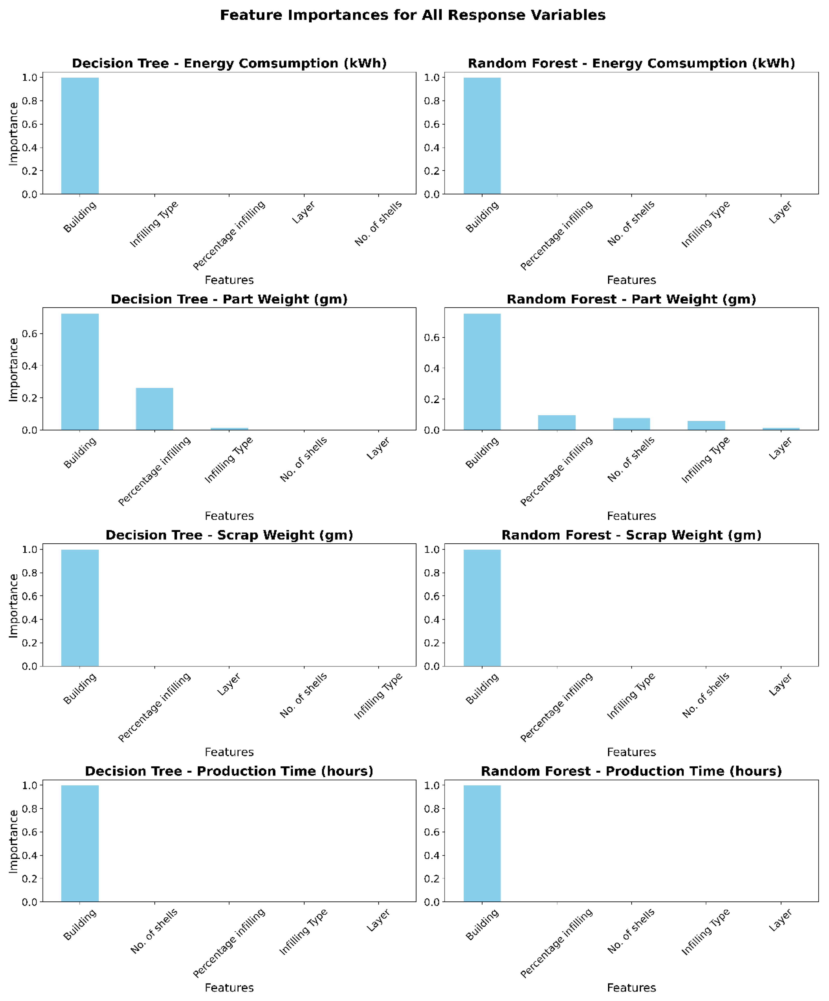
The feature importance plots in Figure 9 consistently identify building orientation as the most critical factor influencing all response variables, including energy consumption shown in Figure 9a, production time Figure 9d, part weight Figure 9b, and scrap weight Figure 9c. Its dominance across the plots reflects its strong influence on the AM process, shaping both energy and material efficiency. While secondary features such as percentage infilling and number of shells occasionally show minor contributions, their importance is far lower, confirming that building orientation is the primary driver of the predictions. This consistent ranking demonstrates the models’ ability to correctly prioritize impactful features while minimizing noise from less relevant ones.
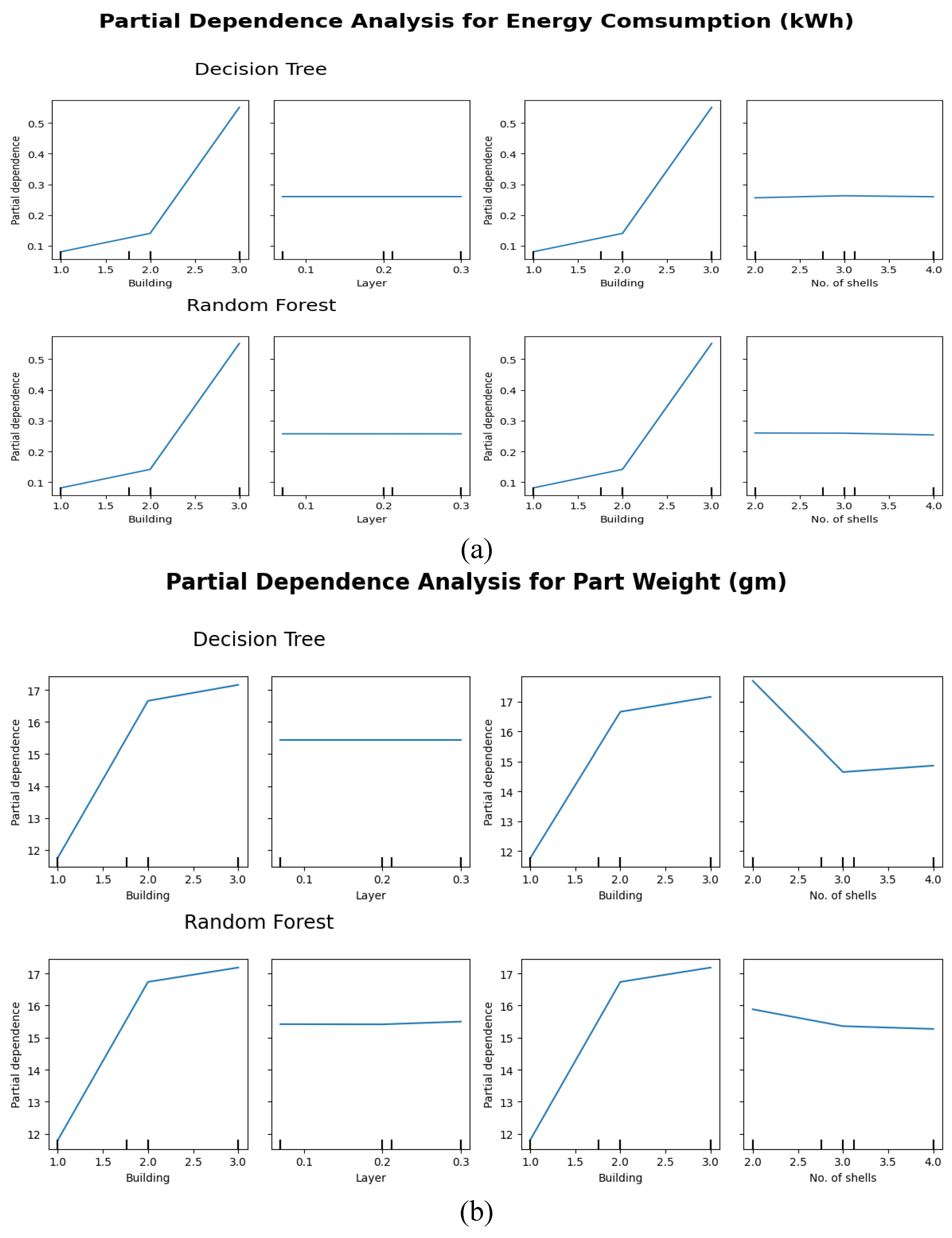
Partial dependence plots in Figure 10 are a visualization technique to interpret ML models by illustrating the marginal effect of a selected feature (or set of features) on the predicted outcome. These plots help isolate and understand the relationship between specific input features and response variables while averaging out effects of other features [34].
In Figure 10, the partial dependence plots reveal a predictable and interpretable relationship between building orientation and the response variables, including energy consumption, printing time, material used, and scrap weight. For energy consumption and production time in Figure 10(a) and (d), the plots exhibit a steady and smooth upward trend as building orientation becomes more complex. This highlights a direct relationship, where increasing orientation complexity demands longer printing times and higher energy usage. In contrast, other parameters, such as layer thickness and the number of shells, show negligible effects on these response variables, as evidenced by their nearly flat trends. This suggests that energy consumption and production time are primarily dictated by building orientation.
Figure 8.
Correlation Analysis: Bar plot (left) and Heatmaps (right).
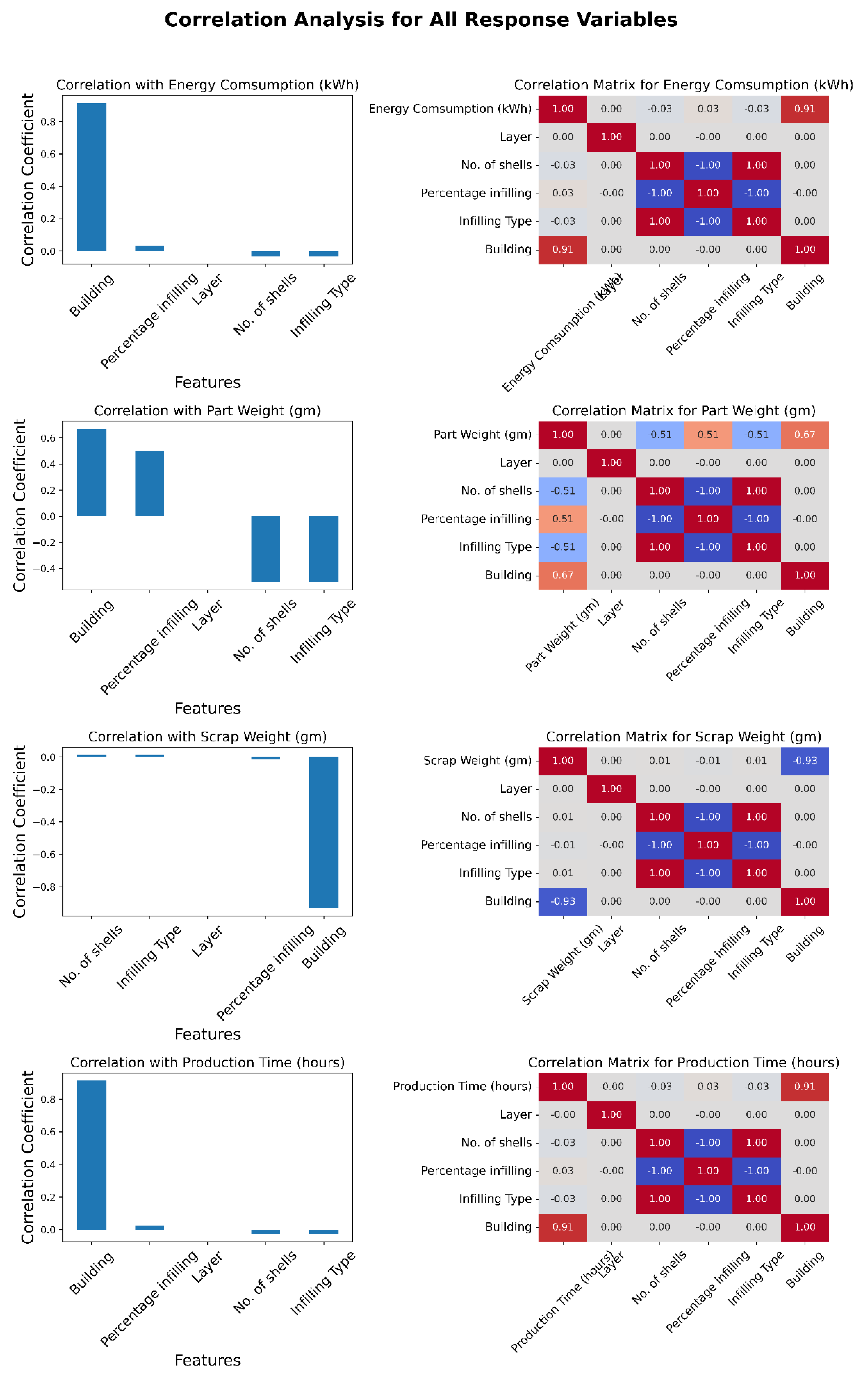
Figure 9.
Feature Analysis of the best performing models: DT (left) and RF (right).
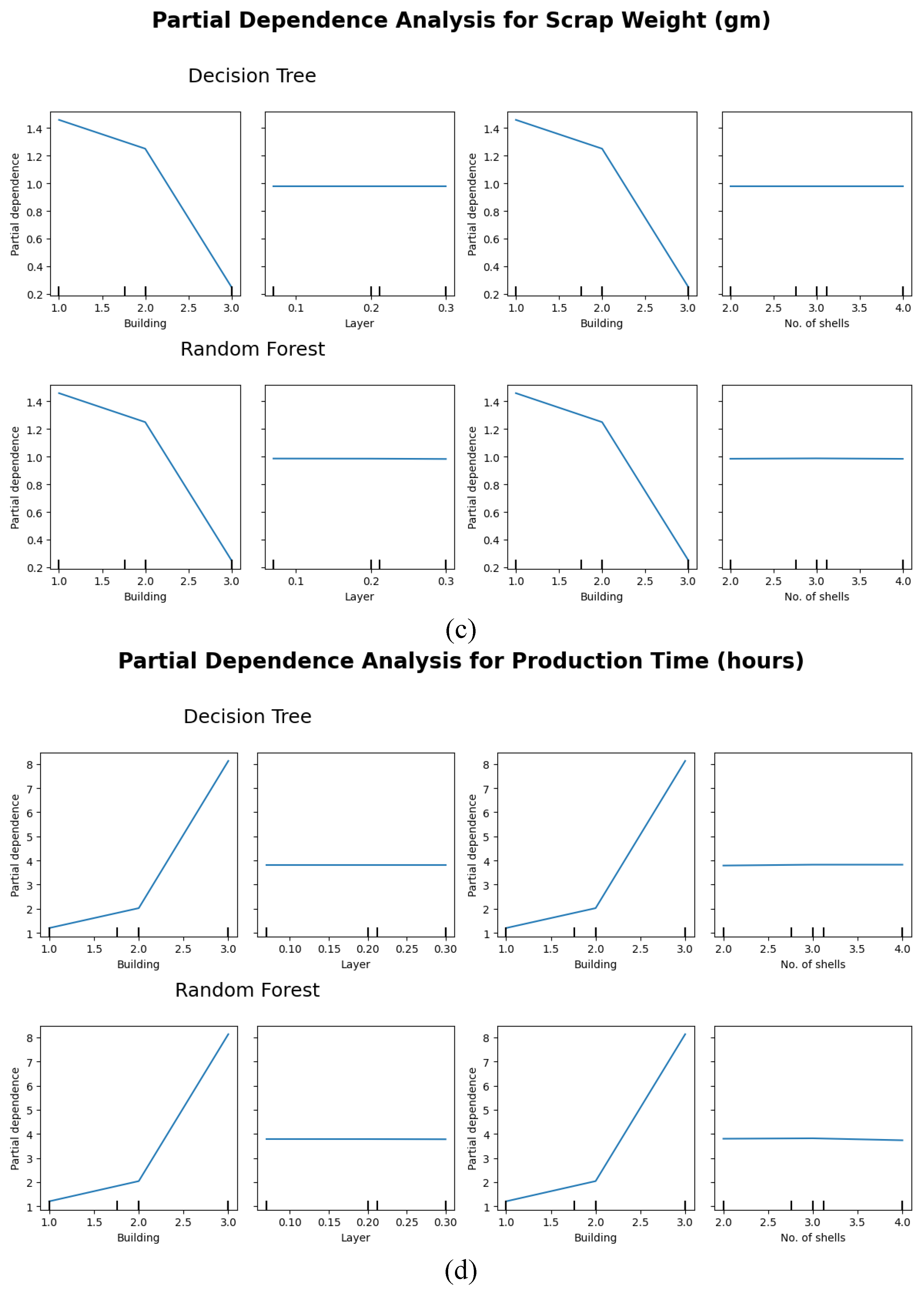
For part weight and scrap weight shown in Figure 10b,c, the influence of building orientation is more nuanced yet significant. The plots indicate a positive trend for part weight, where increasing orientation complexity results in greater part weights due to changes in material distribution patterns. Conversely, the scrap weight demonstrates a consistent decline as the building orientation becomes more optimized, reflecting the ability of certain orientations to reduce waste. While interactions with other parameters, such as percentage infilling, are minimal, they are slightly more pronounced for part weight, where infilling marginally contributes to observed variations. The consistent and smooth gradients observed in the plots across all response variables underscore the robustness of the models in capturing both linear and non-linear dependencies, validating their ability to generalize effectively to complex parameter spaces.
Figure 10.
Partial Dependence plots using DT (top) and RF (bottom) for: (a) Energy Consumption; (b) Part Weight; (c) Scrap Weight; (d) Production Time.
Figure 10.
Partial Dependence plots using DT (top) and RF (bottom) for: (a) Energy Consumption; (b) Part Weight; (c) Scrap Weight; (d) Production Time.
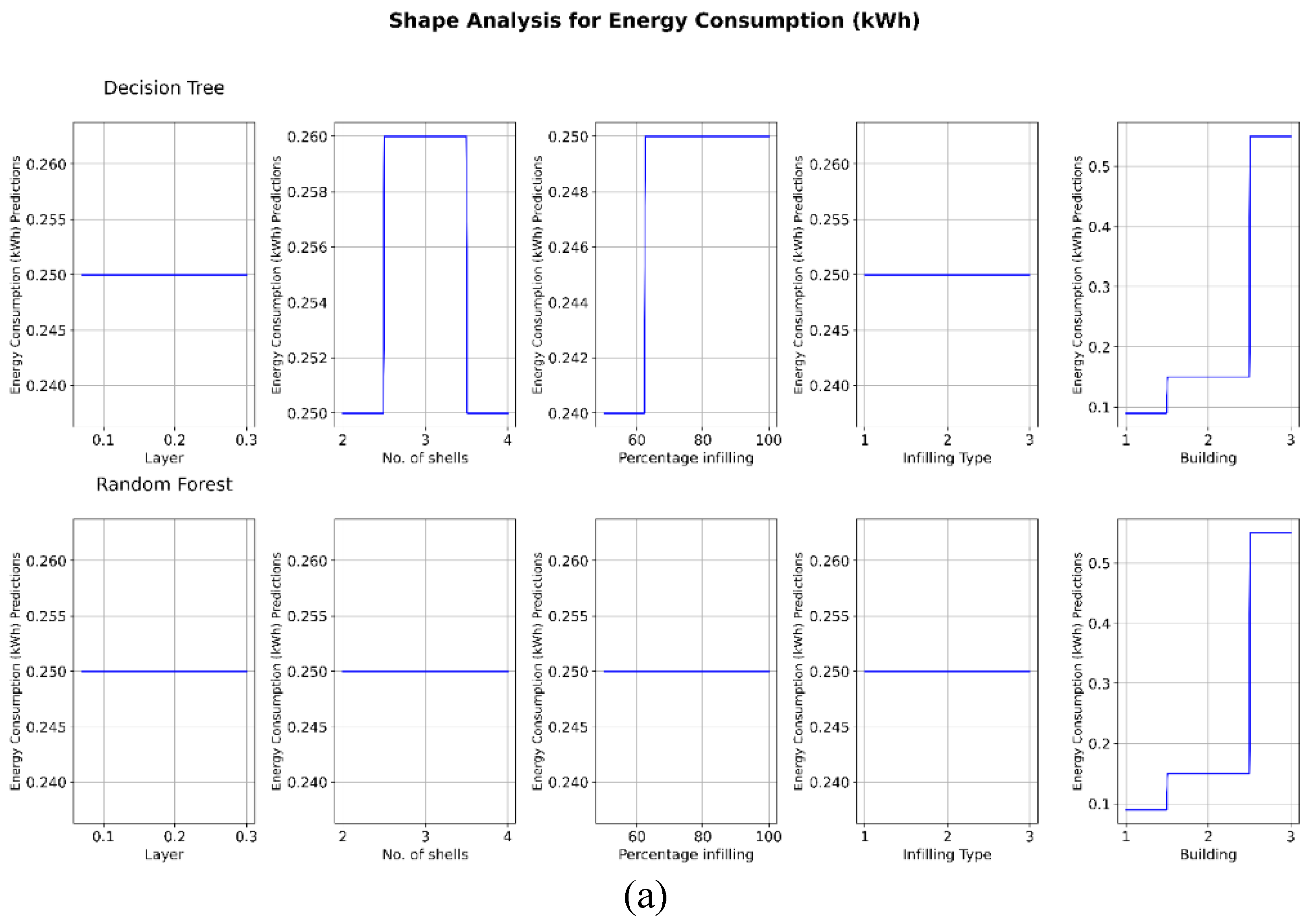
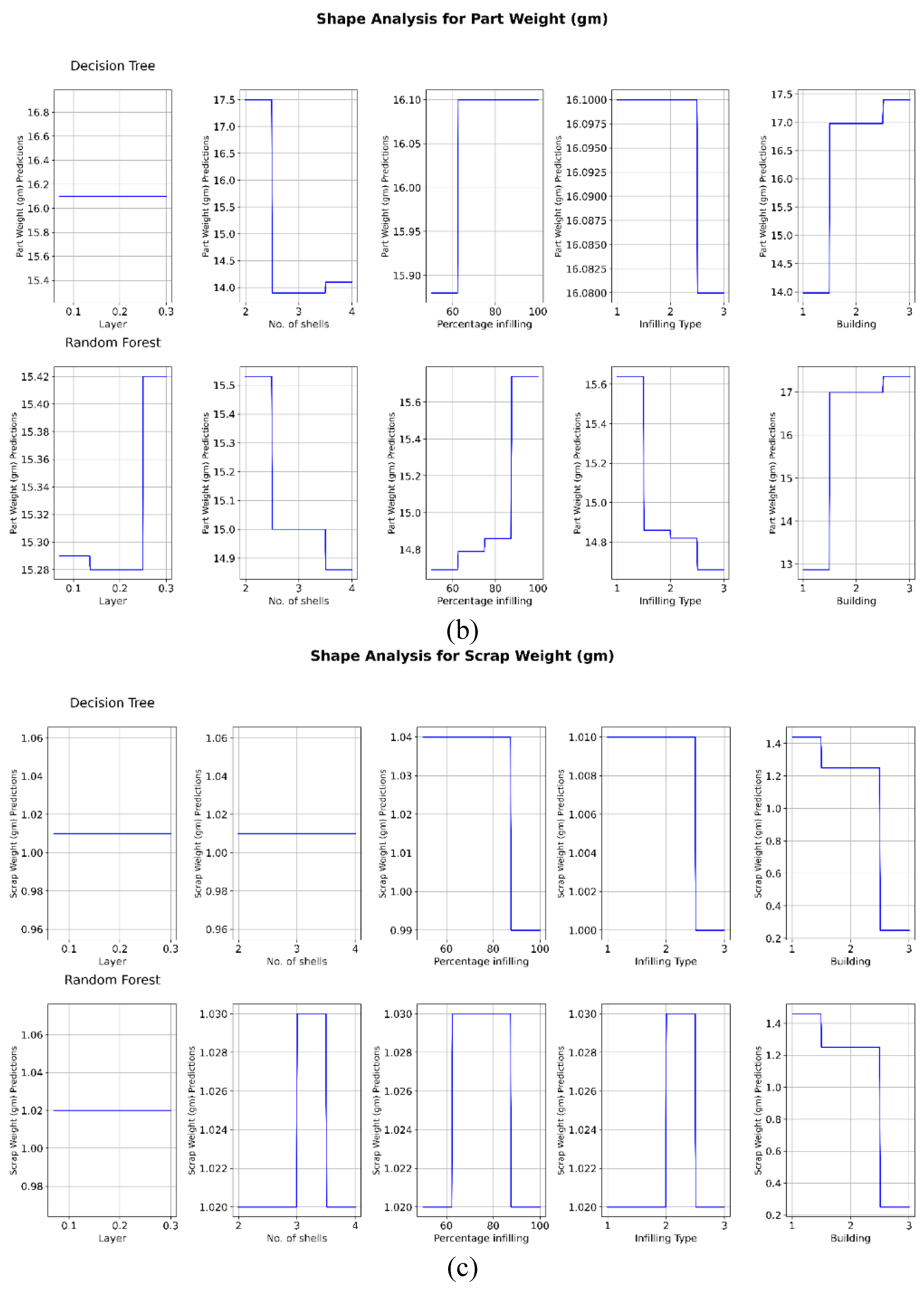
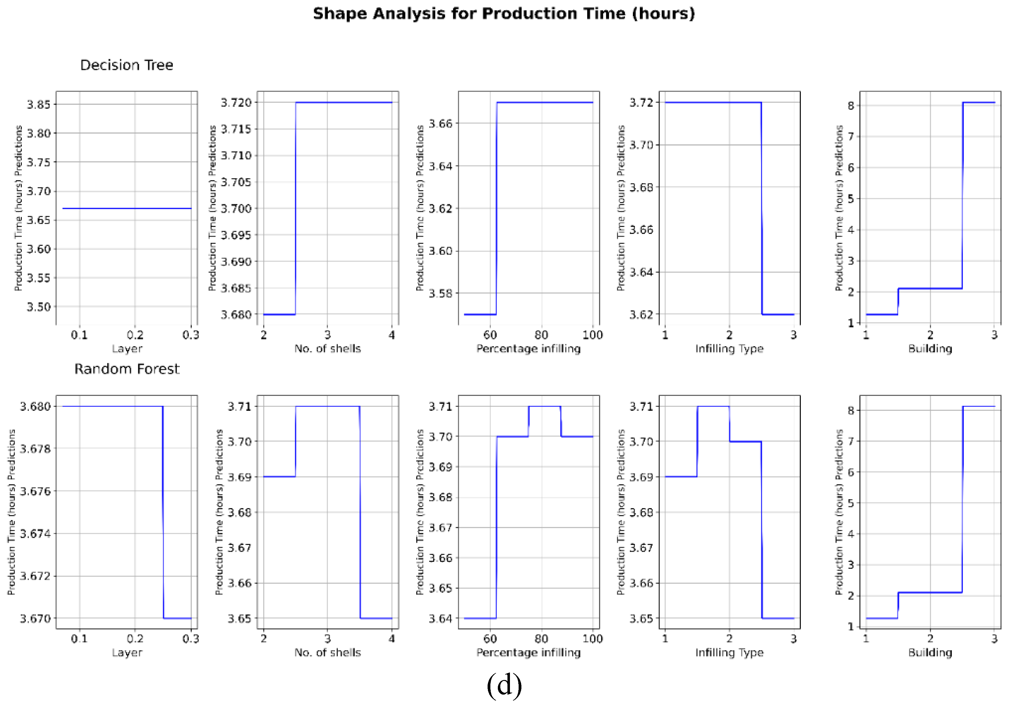
The shape analysis presented in Figure 11, DT (top) and RF (bottom) highlights the robustness of the models by illustrating the relationship between predicted and observed values for energy usage, printing time, material used, and scrap weight [34]. For the energy consumption plots in Figure 11a, the predicted distributions display smooth and consistent trends that align closely with the observed values, especially as building orientation changes. This alignment demonstrates the models' ability to accurately capture the impact of building orientation on energy requirements, with significant shifts in predictions observed as orientation becomes more complex. Similarly, for the production time plots in Figure 11d, the models show a steady increase in predicted values with varying orientation, mirroring the observed trends. This further validates their precision in reflecting dependencies driven by orientation changes.
For the part weight, plots in Figure 11b reveal a stable relationship between predicted and observed values, capturing dependencies influenced by building orientation. The slight variations introduced by secondary parameters like percentage infilling are evident but minimal, reinforcing the models’ focus on the primary contributor i.e. orientation. For the scrap weight plots in Figure 11c, the predicted values show a clear alignment with observed trends, with consistent decreases in scrap weight as the building orientation optimizes. This reflects the models’ capability to minimize material waste effectively through accurate predictions.
Overall, the smooth transitions and alignment in Figure 11 demonstrate that both the models, DT and RF, are well-calibrated and capable of generalizing across different parameter combinations. This further supports their reliability in predicting and optimizing AM processes, contributing to improved efficiency and sustainability.
Figure 11.
Shape Analysis using DT (top) and RF (bottom) for: (a) Energy Consumption; (b) Part Weight; (c) Scrap Weight; (d) Production Time.
Figure 11.
Shape Analysis using DT (top) and RF (bottom) for: (a) Energy Consumption; (b) Part Weight; (c) Scrap Weight; (d) Production Time.
The results demonstrate the exceptional performance of the DT and RF models in predicting and optimizing response variables for AM. Building orientation consistently emerges as the dominant factor influencing energy usage, printing time, material used, and scrap weight, as highlighted by feature importance rankings and partial dependence plots. The models capture clear, interpretable relationships, showing that increasing orientation complexity leads to higher energy usage and production time, increased part weight, and reduced scrap. Secondary features, such as percentage infilling and the number of shells, play minor roles, contributing only marginally in specific cases. The smooth gradients and alignment between predicted and observed distributions validate the robustness and generalizability of DT and RF as dominant ML models. Together, these findings underscore the models’ capability in both prediction and optimization, reinforcing their utility in enhancing AM processes for improved efficiency and sustainability.
5. Conclusions
This paper evaluates ML models to identify the most suitable model to accurately predicting sustainability outcomes of AM processes. The DT and RF ML models successfully captures relationships between key AM parameters such as layer thickness, number of shells, build orientation, infill type, and infill percentage and sustainability metrics including energy usage, part weight, scrap material, and printing time. By leveraging these models, it becomes possible to optimize AM parameters for manufacturers to obtain sustainability outcomes in a more efficient and targeted manner. This approach not only minimizes resource consumption but also improves energy efficiency and material utilization, contributing to both environmental and economic sustainability in AM. Ultimately, ML offers a powerful tool for controlling and enhancing the sustainability of AM processes, allowing for more sustainable manufacturing practices in the future.
The research is limited by its focus on the specific material, parameters, and AM technique, which may not fully capture the broader range of possibilities in AM. Expanding the scope to include more materials and methods would provide a more comprehensive understanding of AM's sustainability.
Authors’ Contributions The authors contributed equally to the study.
Funding This work is supported by the Discovery Grants from the Natural Sciences and Engineering Research Council (NSERC) of Canada and Mitacs Lab2Market program.
Data Availability The experimental data are provided in Figure 4.
Abbreviations
| AM FDM CM |
Additive Manufacturing Fused Deposition Modelling Conventional Manufacturing |
| LCA LCC ML LinReg DT RF GB R² MAE MSE |
Life Cycle Assessment Life Cycle Cost Machine Learning Linear Regression Decision Tree Random Forest Gradient Boosting Coefficient of Determination Mean Absolute Error Mean Squared Error |
References
- Panagiotopoulou, V.C.; Stavropoulos, P.; Chryssolouris, G. A Critical Review on the Environmental Impact of Manufacturing: A Holistic Perspective. The International Journal of Advanced Manufacturing Technology 2022, 118, 603–625. [Google Scholar] [CrossRef]
- Shah, H.H.; Tregambi, C.; Bareschino, P.; Pepe, F. Environmental and Economic Sustainability of Additive Manufacturing: A Systematic Literature Review. Sustain Prod Consum 2024, 51, 628–643. [Google Scholar] [CrossRef]
- Adekanye, S.A.; Mahamood, R.M.; Akinlabi, E.T.; Owolabi, M.G. Additive Manufacturing: The Future of Manufacturing. Materiali in Tehnologije 2017, 51, 709–715. [Google Scholar] [CrossRef]
- Bandyopadhyay, A.; Bose, S. ADDITIVE MANUFACTURING; Second edition.; CRC PRESS: BOCA RATON, 2019; ISBN 1-5231-3442-9. [Google Scholar]
- Singh, R.; Davim, J.P. Additive Manufacturing: Applications and Innovations; Manufacturing Design and Technology; First edition.; CRC Press: Boca Raton, FL, 2018; ISBN 1-351-68666-6. [Google Scholar]
- Hidalgo-Carvajal, D.; Munoz, A.H.; Garrido-Gonzalez, J.J.; Carrasco-Gallego, R.; Montero, V.A. Recycled PLA for 3D Printing: A Comparison of Recycled PLA Filaments from Waste of Different Origins after Repeated Cycles of Extrusion. Polymers (Basel) 2023, 15. [Google Scholar] [CrossRef] [PubMed]
- Report of the World Commission on Environment and Development (a/42/427); 1987.
- Meng, L.; McWilliams, B.; Jarosinski, W.; Park, H.-Y.; Jung, Y.-G.; Lee, J.; Zhang, J. Machine Learning in Additive Manufacturing: A Review. JOM 2020, 72, 2363–2377. [Google Scholar] [CrossRef]
- Shehbaz, W.; Peng, Q. Selection and Optimization of Additive Manufacturing Process Parameters Using Machine Learning: A Review; 2024.
- Swetha, R.; Siva Rama Krishna, L.; Hari Sai Kiran, B.; Ravinder Reddy, P.; Venkatesh, S. Comparative Study on Life Cycle Assessment of Components Produced by Additive and Conventional Manufacturing Process. Mater Today Proc 2022, 62, 4332–4340. [Google Scholar] [CrossRef]
- Výtisk, J.; Honus, S.; Kočí, V.; Pagáč, M.; Hajnyš, J.; Vujanovic, M.; Vrtek, M. Comparative Study by Life Cycle Assessment of an Air Ejector and Orifice Plate for Experimental Measuring Stand Manufactured by Conventional Manufacturing and Additive Manufacturing. Sustainable Materials and Technologies 2022, 32, e00431. [Google Scholar] [CrossRef]
- Solaimani, S.; Parandian, A.; Nabiollahi, N. A Holistic View on Sustainability in Additive and Subtractive Manufacturing: A Comparative Empirical Study of Eyewear Production Systems. Sustainability 2021, 13. [Google Scholar] [CrossRef]
- Kokare, S.; Oliveira, J.P.; Godina, R. A LCA and LCC Analysis of Pure Subtractive Manufacturing, Wire Arc Additive Manufacturing, and Selective Laser Melting Approaches. J Manuf Process 2023, 101, 67–85. [Google Scholar] [CrossRef]
- Khalid, M.; Peng, Q. Investigation of Printing Parameters of Additive Manufacturing Process for Sustainability Using Design of Experiments. JOURNAL OF MECHANICAL DESIGN 2021, 143. [Google Scholar] [CrossRef]
- Dudek, P.; Zagórski, K. Cost, Resources, and Energy Efficiency of Additive Manufacturing. In Proceedings of the E3S WEB CONF; E D P Sciences: CEDEX A, 2017; Vol. 14, p. 1040. [Google Scholar]
- Rejeski, D.; Zhao, F.; Huang, Y. Research Needs and Recommendations on Environmental Implications of Additive Manufacturing. Addit Manuf 2018, 19, 21–28. [Google Scholar] [CrossRef]
- Simon, T.R.; Lee, W.J.; Spurgeon, B.E.; Boor, B.E.; Zhao, F. An Experimental Study on the Energy Consumption and Emission Profile of Fused Deposition Modeling Process. Procedia Manuf 2018, 26, 920–928. [Google Scholar] [CrossRef]
- Liu, Z.Y.; Li, C.; Fang, X.Y.; Guo, Y.B. Energy Consumption in Additive Manufacturing of Metal Parts. Procedia Manuf 2018, 26, 834–845. [Google Scholar] [CrossRef]
- Nagarajan, H.P.N.; Haapala, K.R. Environmental Performance Evaluation of Direct Metal Laser Sintering through Exergy Analysis. Procedia Manuf 2017, 10, 957–967. [Google Scholar] [CrossRef]
- Schneevogt, H.; Stelzner, K.; Yilmaz, B.; Abali, B.E.; Klunker, A.; Völlmecke, C. Sustainability in Additive Manufacturing: Exploring the Mechanical Potential of Recycled PET Filaments. Composites and Advanced Materials 2021, 30, 26349833211000064. [Google Scholar] [CrossRef]
- Tang, Y.; Mak, K.; Zhao, Y.F. A Framework to Reduce Product Environmental Impact through Design Optimization for Additive Manufacturing. J Clean Prod 2016, 137, 1560–1572. [Google Scholar] [CrossRef]
- Tavares, T.; Filho, M.; Ganga, G.; Callefi, M.H. The Relationship between Additive Manufacturing and Circular Economy: A Sistematic Review. Independent Journal of Management & Production 2020, 11, 1648. [Google Scholar] [CrossRef]
- Huu, P.N.; Van, D.P.; Xuan, T.H.; Ilani, M.A.; Trong, L.N.; Thanh, H.H.; Chi, T.N. Review: Enhancing Additive Digital Manufacturing with Supervised Classification Machine Learning Algorithms. The International Journal of Advanced Manufacturing Technology 2024, 133, 1027–1043. [Google Scholar] [CrossRef]
- Nasrin, T.; Pourkamali-Anaraki, F.; Peterson, A.M. Application of Machine Learning in Polymer Additive Manufacturing: A Review. JOURNAL OF POLYMER SCIENCE 2023. [Google Scholar] [CrossRef]
- Mishra, A.; Jatti, V.S.; Sefene, E.M.; Jatti, A. V; Sisay, A.D.; Khedkar, N.K.; Salunkhe, S.; Pagac, M.; Nasr, E.S.A. Machine Learning-Assisted Pattern Recognition Algorithms for Estimating Ultimate Tensile Strength in Fused Deposition Modelled Polylactic Acid Specimens. MATERIALS TECHNOLOGY 2024, 39. [Google Scholar] [CrossRef]
- Ziadia, A.; Mohamed, H.; Kelouwani, S. Machine Learning Study of the Effect of Process Parameters on Tensile Strength of FFF PLA and PLA-CF. Eng 2023, 4, 2741–2763. [Google Scholar] [CrossRef]
- Maleki, E.; Bagherifard, S.; Guagliano, M. Application of Artificial Intelligence to Optimize the Process Parameters Effects on Tensile Properties of Ti-6Al-4V Fabricated by Laser Powder-Bed Fusion. International Journal of Mechanics and Materials in Design 2022, 18, 199–222. [Google Scholar] [CrossRef]
- Chigilipalli, B.K.; Veeramani, A. A Machine Learning Approach for the Prediction of Tensile Deformation Behavior in Wire Arc Additive Manufacturing. IJIDEM 2023. [Google Scholar] [CrossRef]
- Ege, D.; Sertturk, S.; Acarkan, B.; Ademoglu, A. Machine Learning Models to Predict the Relationship between Printing Parameters and Tensile Strength of 3D Poly (Lactic Acid) Scaffolds for Tissue Engineering Applications Machine Learning Models to Predict the Relationship between Printing Parameters and Tensile Strength of 3D Poly (Lactic Acid) Scaffolds for Tissue Engineering Applications. Biomed Phys Eng Express 2023, 9. [Google Scholar] [CrossRef]
- Agarwal, R.; Singh, J.; Gupta, V. Predicting the Compressive Strength of Additively Manufactured PLA-Based Orthopedic Bone Screws: A Machine Learning Framework. Polym Compos 2022, 43, 5663–5674. [Google Scholar] [CrossRef]
- Zhang, Z.; Shi, J.; Yu, T.; Santomauro, A.; Gordon, A.; Gou, J.; Wu, D. Predicting Flexural Strength of Additively Manufactured Continuous Carbon Fiber-Reinforced Polymer Composites Using Machine Learning. J Comput Inf Sci Eng 2020, 20, 1–32. [Google Scholar] [CrossRef]
- Chen, J.; Liu, Y. Neural Optimization Machine: A Neural Network Approach for Optimization; 2022.
- Chen, J.; Liu, Y.M. Neural Optimization Machine: A Neural Network Approach for Optimization and Its Application in Additive Manufacturing with Physics-Guided Learning. Philosophical Transactions of the Royal Society A-Mathematical Physical and Engineering Sciences 2023, 381. [Google Scholar] [CrossRef]
- Kharate, N.; Anerao, P.; Kulkarni, A.; Abdullah, M. Explainable AI Techniques for Comprehensive Analysis of the Relationship between Process Parameters and Material Properties in FDM-Based 3D-Printed Biocomposites. Journal of Manufacturing and Materials Processing 2024, 8. [Google Scholar] [CrossRef]
- Chang, L.-K.; Chen, R.-S.; Tsai, M.-C.; Lee, R.-M.; Lin, C.-C.; Huang, J.-C.; Chang, T.-W.; Horng, M.-H. Machine Learning Applied to Property Prediction of Metal Additive Manufacturing Products with Textural Features Extraction. The International Journal of Advanced Manufacturing Technology 2024, 132, 83–98. [Google Scholar] [CrossRef]
- Jayawardane, H.; Davies, I.J.; Gamage, J.R.; John, M.; Biswas, W.K. Sustainability Perspectives – a Review of Additive and Subtractive Manufacturing. Sustainable Manufacturing and Service Economics 2023, 2, 100015. [Google Scholar] [CrossRef]
- Mani, M.; Lyons, K.W.; Gupta, S.K. Sustainability Characterization for Additive Manufacturing. J Res Natl Inst Stand Technol 2014, 119, 419–428. [Google Scholar] [CrossRef] [PubMed]
- Ford, S.; Despeisse, M. Additive Manufacturing and Sustainability: An Exploratory Study of the Advantages and Challenges. J Clean Prod 2016, 137, 1573–1587. [Google Scholar] [CrossRef]
- Akbari, P.; Zamani, M.; Mostafaei, A. Machine Learning Prediction of Mechanical Properties in Metal Additive Manufacturing. Addit Manuf 2024, 91, 104320. [Google Scholar] [CrossRef]
Figure 7.
Performance score of DT vs RF on training and testing datasets.
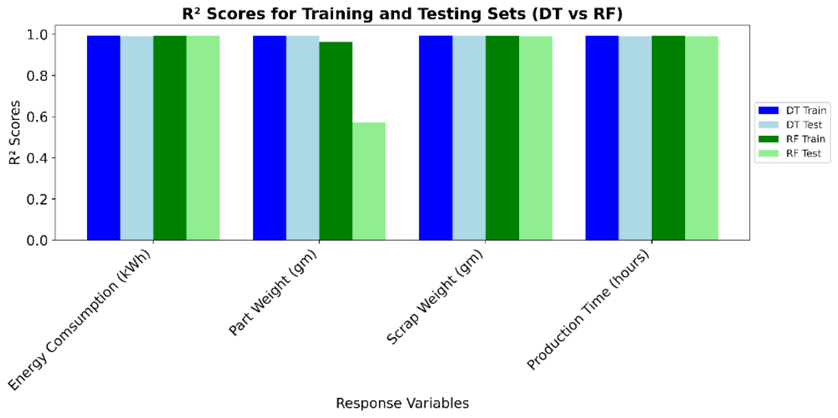

Table 1.
Hyperparameter configuration for DT and RF ML models.
| Model | Hyperparameters |
| Decision Tree | Random-state=42 |
| Random Forest | n-estimators=100, random-state=42 |
| Train-Test-Split | Test-size=0.2, random-state=42 |
| minimize (L-BFGS-B) | method='L-BFGS-B' |
Table 2.
The three levels of Process Parameters.
| Process Parameters | Levels | ||
| Layer thickness | 0.07 | 0.2 | 0.3 |
| Number of shells | 2 | 3 | 4 |
| Infill percentage | 50 | 75 | 100 |
| Infill type | Cross | Diamond | Honeycomb |
| Build orientation | Flat | On-edge | Up right |
Table 3.
Optimized Parameters for the best performing ML models.
| Model | Layer | No. of Shells | Infill % | Infill Type |
Build Orientation |
EC (kWh) | PW (gm) | SW (gm) | PT (hours) | |
| DT | 0.2 | 3 | 75 | Diamond | On-edge | 0.140 | 16.10 | 1.2 | 2.1 | |
| RF | 0.2 | 3 | 75 | Diamond | On-edge | 0.139 | 16.09 | 1.2 | 2 | |
Disclaimer/Publisher’s Note: The statements, opinions and data contained in all publications are solely those of the individual author(s) and contributor(s) and not of MDPI and/or the editor(s). MDPI and/or the editor(s) disclaim responsibility for any injury to people or property resulting from any ideas, methods, instructions or products referred to in the content. |
© 2025 by the authors. Licensee MDPI, Basel, Switzerland. This article is an open access article distributed under the terms and conditions of the Creative Commons Attribution (CC BY) license (https://creativecommons.org/licenses/by/4.0/).
Copyright: This open access article is published under a Creative Commons CC BY 4.0 license, which permit the free download, distribution, and reuse, provided that the author and preprint are cited in any reuse.


