Submitted:
20 December 2024
Posted:
24 December 2024
You are already at the latest version
Abstract
One of the most flexible assets in the financial markets is the options, the flexibility makes it possible to create virtually unlimited strategies among different underlying assets, and combinations, contrary to the stock market, where the mechanism to sell or buy is relatively simple, other elements, like time can play against the trader. The derivative market could be overwhelming considering the broad al-ternatives, with high entry barriers and a steep learning curve. The new traders try to jump these bar-riers without a plan, hurrying to place trades that follow their emotions, and losing money along the process, as the best alternative to learn from trial and error. This research proposes an options trading framework that can help reduce this gap and profit from time decay.
Keywords:
1. Introduction
2. Literature Review
- Relative Strength Index (RSI).
- Moving Average Convergence Divergence (MACD).
- Bollinger Bands (BB).
- Directional Movement Index (DI+, DI- and ADX).
2. Theoretical Framework
2.1. Options Strategies
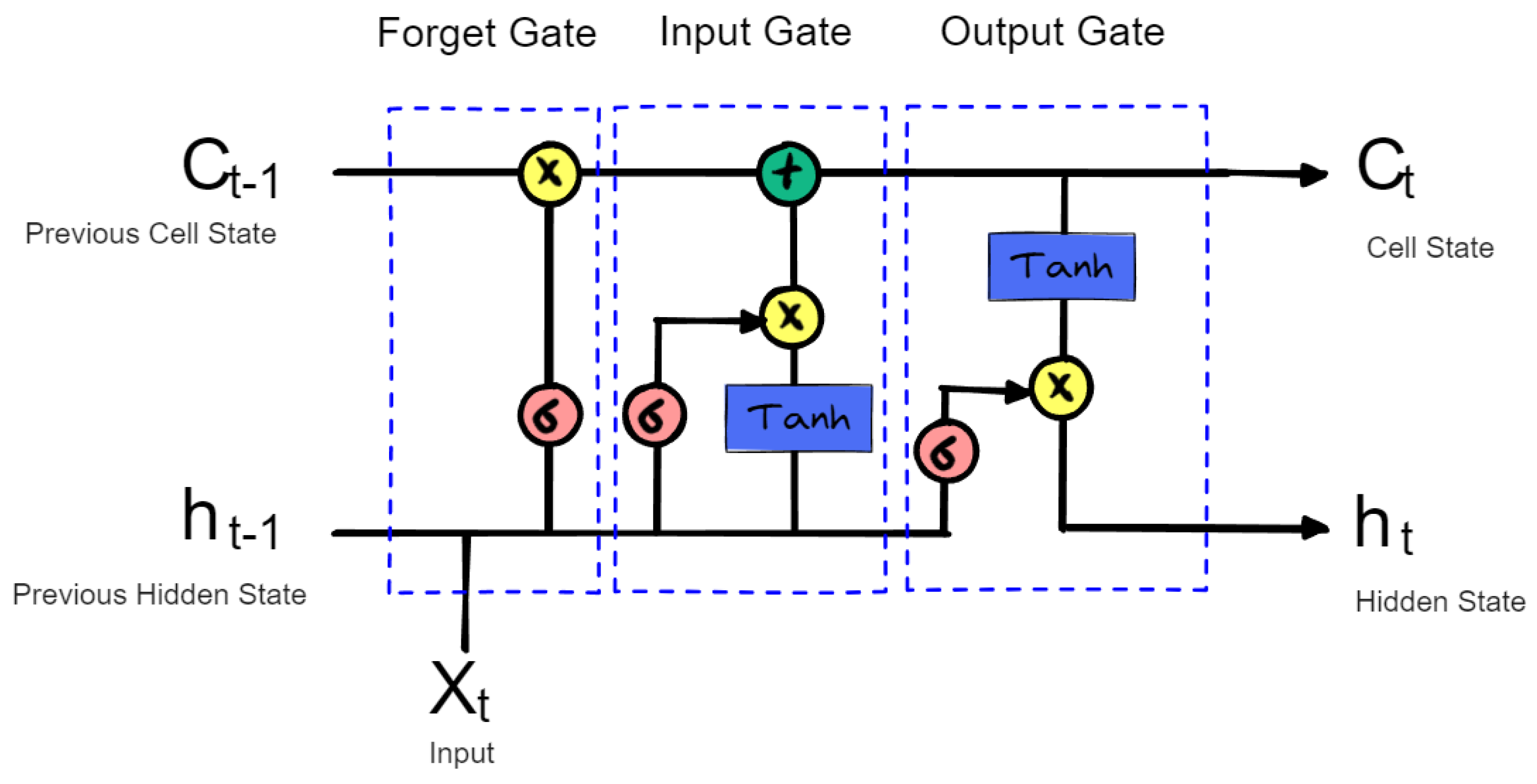
2.2. LSTM-CNN
- Forget gate: This is responsible for deciding the information that should not be in the cell state .
- Input gate: This gate decides which information is stored in the memory.
- Output cell: It is responsible for the information that is shown from the cell state at time .
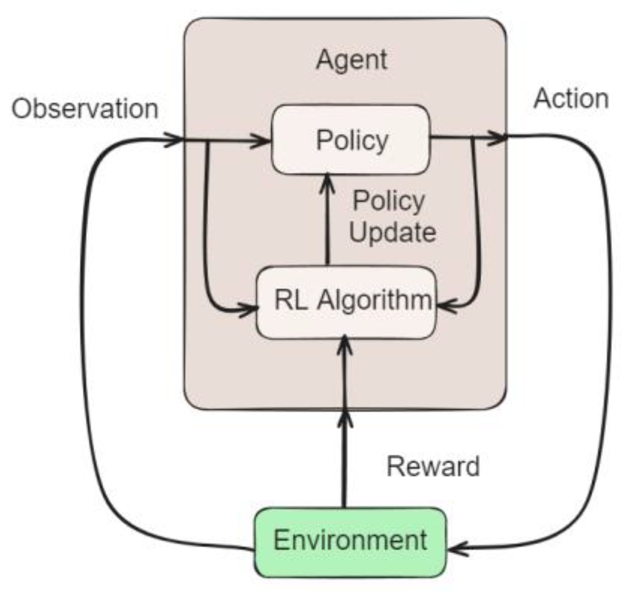
2.3. Reinforcement Learning
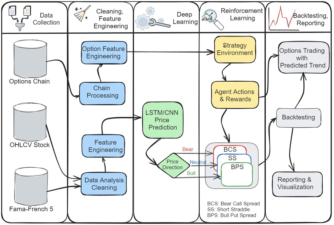
3. Methodology
3.1. Data Collection
3.2. Feature Engineering
- Relative Strength Index (RSI): This momentum indicator will give us insights about the uptrend or downtrend in the price, the direction and strength in price movement. The default configuration is to use 14 periods. It has a range value between 0 and 100.
- Moving Average Convergence Divergence (MACD): This is another momentum indicator. It is calculated by subtracting 12 and 26 EMA periods on closing prices. It identifies strengths, directions, and momentum in stock prices.
- Bollinger Bands (BB higher, low): The BB are used to know if the prices are high and low in relation to each other. This indicator can measure volatility and also trends in the stock movement.
- Directional Movement Index (DI+, DI- and ADX): These indicators also measure strength and direction, it is used to confirm trends, and it can be used together with ADX (Average Directional Index) to show momentum.
- Exponential Moving Average (EMA): This indicator gives us information about price change direction, values from 30 and 50 days are considered.
- On-Balance Volume (OBV): OBV helps to confirm uptrend or downtrend as regards price increase or the opposite, basically measuring the buying and selling pressure.
- Accumulation/Distribution Line (ADL): This measures the cumulative flow of money in and out of a stock, it belongs also to the volume group indicators.
- Aroon Indicator: It identifies changes in price trends, it is composed of two lines and their interactions give information about the strength of uptrend and downtrend.
- Average True Range (ATR): This is primarily used to measure volatility or average price range over time.
- CBOE Volatility Index (VIX): This reflects the market's expectations about volatility over the next 30 days, the volatility can be seen as a measure of risk in the market.
- Market Risk (Mkt-RF): This is the market excess returns over the risk-free rate (market premium).
- Size Factor (SMB - Small Minus Big): The returns between small-cap and large-cap stocks (size premium).
- Value Factor (HML - High Minus Low): The return spread between value and growth stocks (value premium).
- Profitability Factor (RMW - Robust Minus Weak): The return between stocks of companies with strong profitability and those with weak profitability.
- Investment Factor (CMA - Conservative Minus Aggressive): The return difference between conservative stocks investment companies and those that invest aggressively.
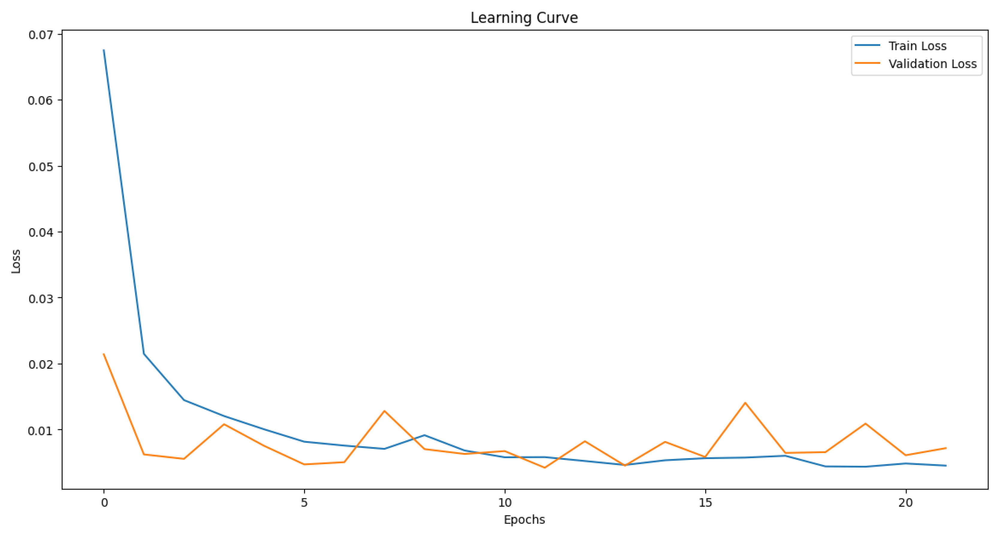
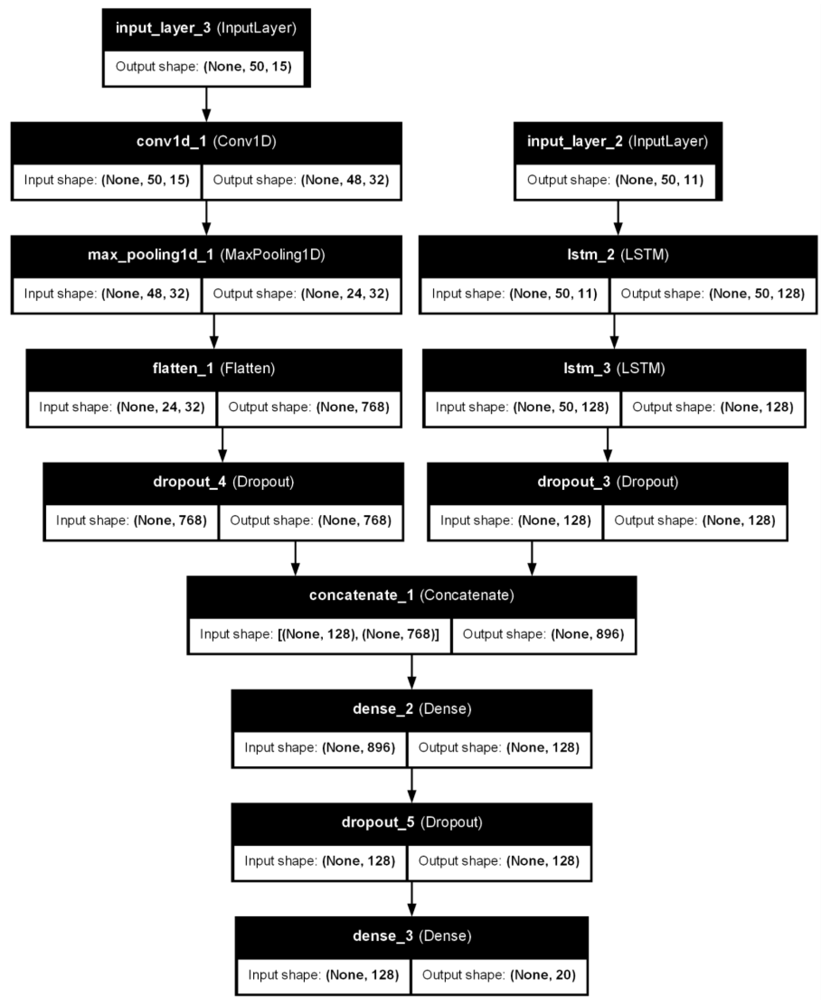
3.3 Deep Learning
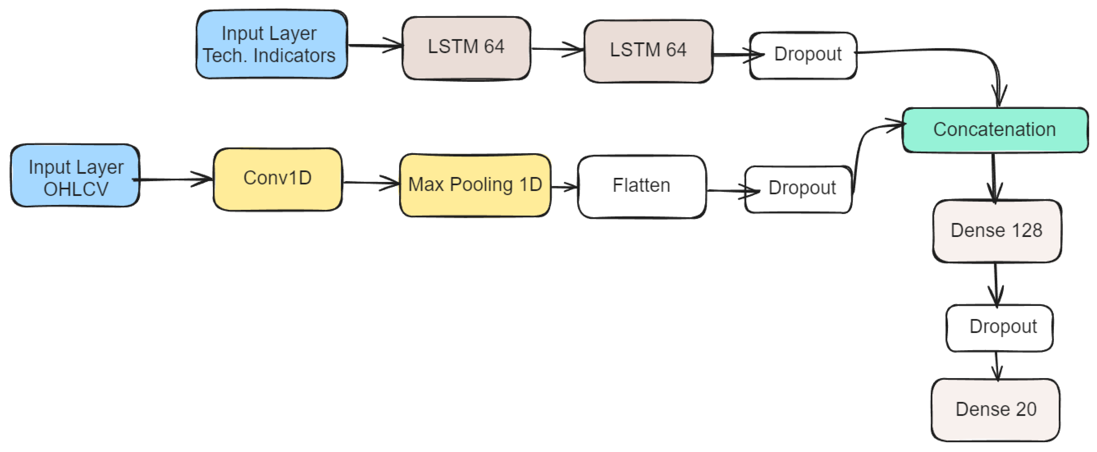
- Inputs: Stock data OHLCV (5), VIX, Fama-French (5) factors, and technical indicators (15).
- LSTM Leg (OHLCV): Two LSTM layers with 64 units each and a Dropout layer 0.2 to avoid overfitting.
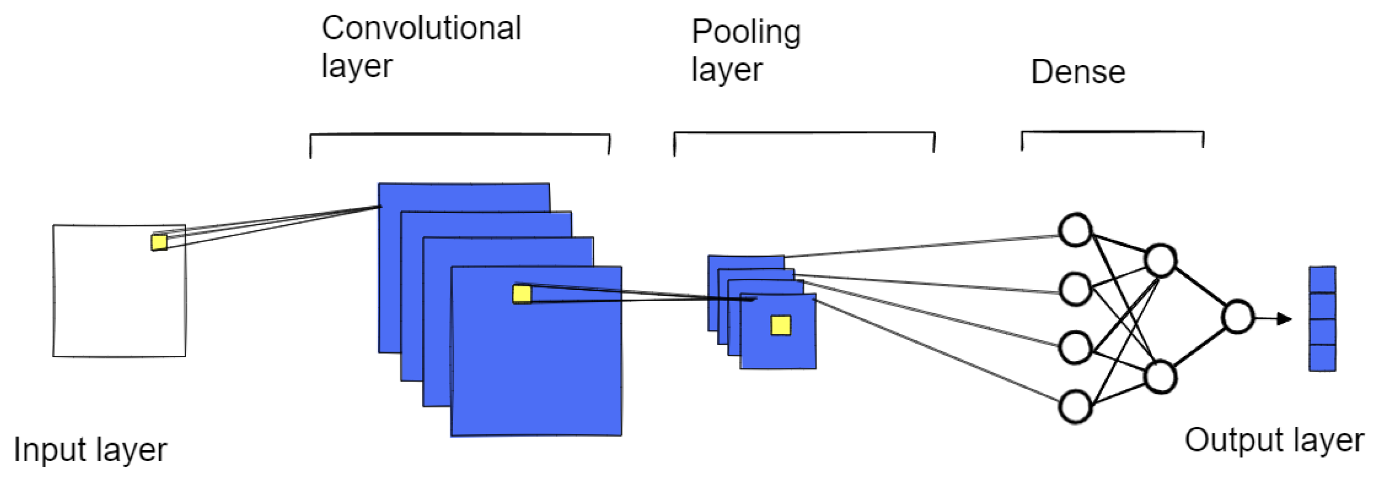
- CNN Leg (technical indicators): It is composed of Conv1D layer 32 filters and a kernel size of 3, MaxPooling1D layer with a pool size of 2, Flatten layer to convert the 2D output to 1D, and Dropout with a rate of 0.2.
- Legs concatenation and Output: These previous two legs are concatenated, and connected with a Dense layer of 128 units, then Dropout 0.2, and finally output Dense layer with 20 (days to be forecasted).
3.4. Historical Options Chain Analysis
- Analyze the historical options chains for AAPL and filter out the weekly expiry chains.
- Run exploratory data analysis to check and fix: The null values records, column names, data types of the columns, and zero volume records.
- For a given strategy, prepare the spreads/legs within the same expiry date and quote date for each combination of the lower and higher strike with the DTE, Greeks, IV, etc.
3.5. Feature Engineering for the Historical Options Chains
- Net Credit: It is the difference between the bid price and the asking price of the legs.
- Max Profit: In the case of selling strategies, the maximum profit is always the net credit received when the trader enters the trade.
- Max Loss: The maximum loss or strategy margin is the difference between both strikes and credit received.
- Net Delta: It is the difference between the delta values of both legs.
- Probability of expiring worthless; As delta also signifies the probability of an option strategy expiring ITM (In the Money), the inverse probability of Net Delta tells the probability of expiring worthless.
- Margin paid: This is the margin paid to the broker, since the strategies are short, so margin requirements would be higher and could be different in each strategy type.
- Expected Return on Margin: This is the expected return for the paid margin, which is basically the max profit divided by the paid margin.
3.6. Strategy Execution
3.6.1. Environment Setup
- Action 1 (Open): Rewards positively high probability if expiring worthless and substantial expected return on the paid margin and days to expiration between 15 and 45.
- Action 0 (Avoid): Else reward negative for the rest of combinations.
4. Results
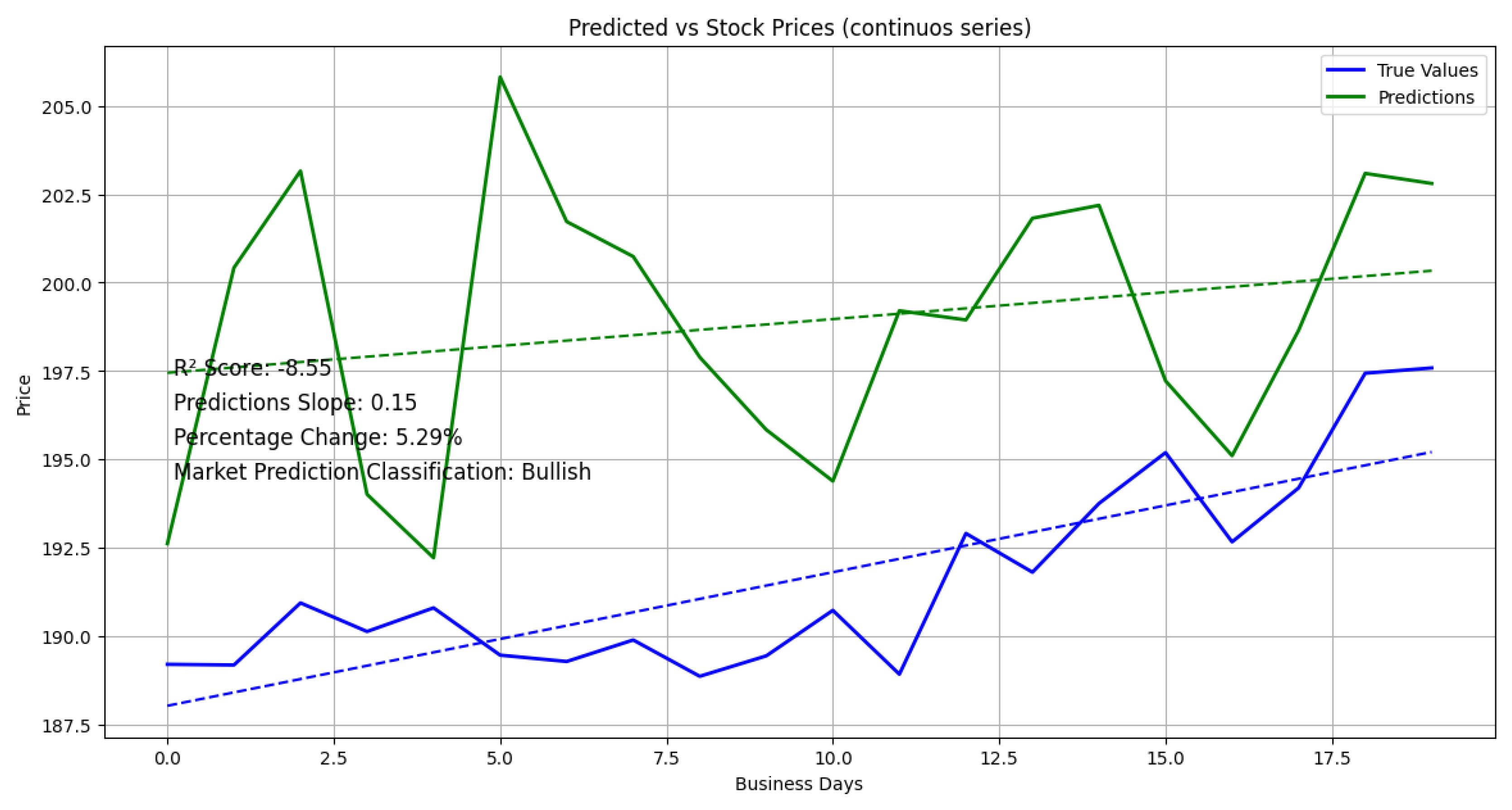
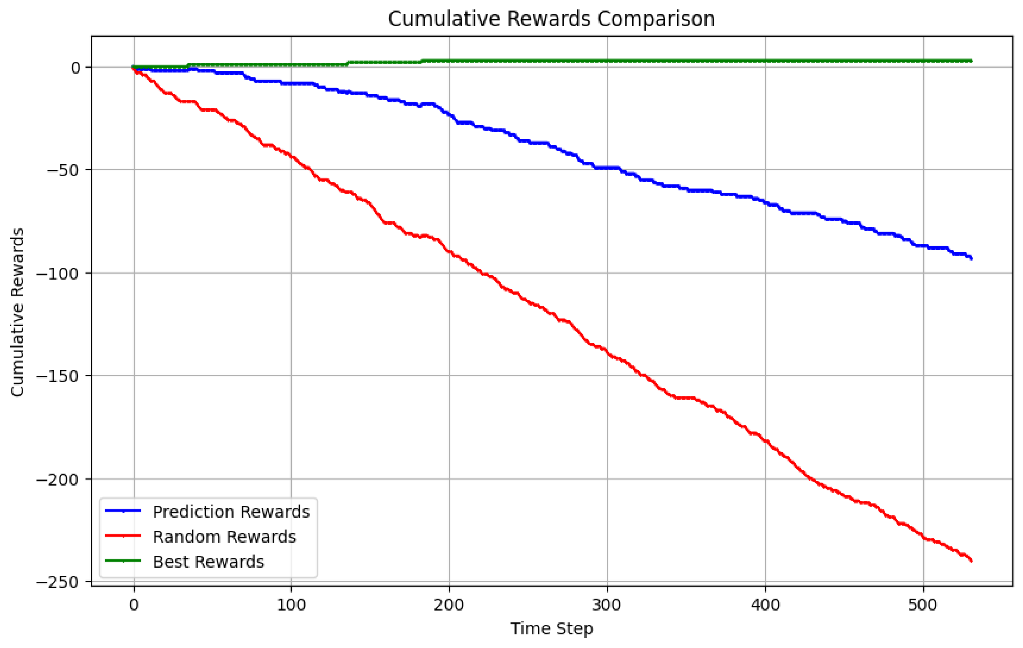
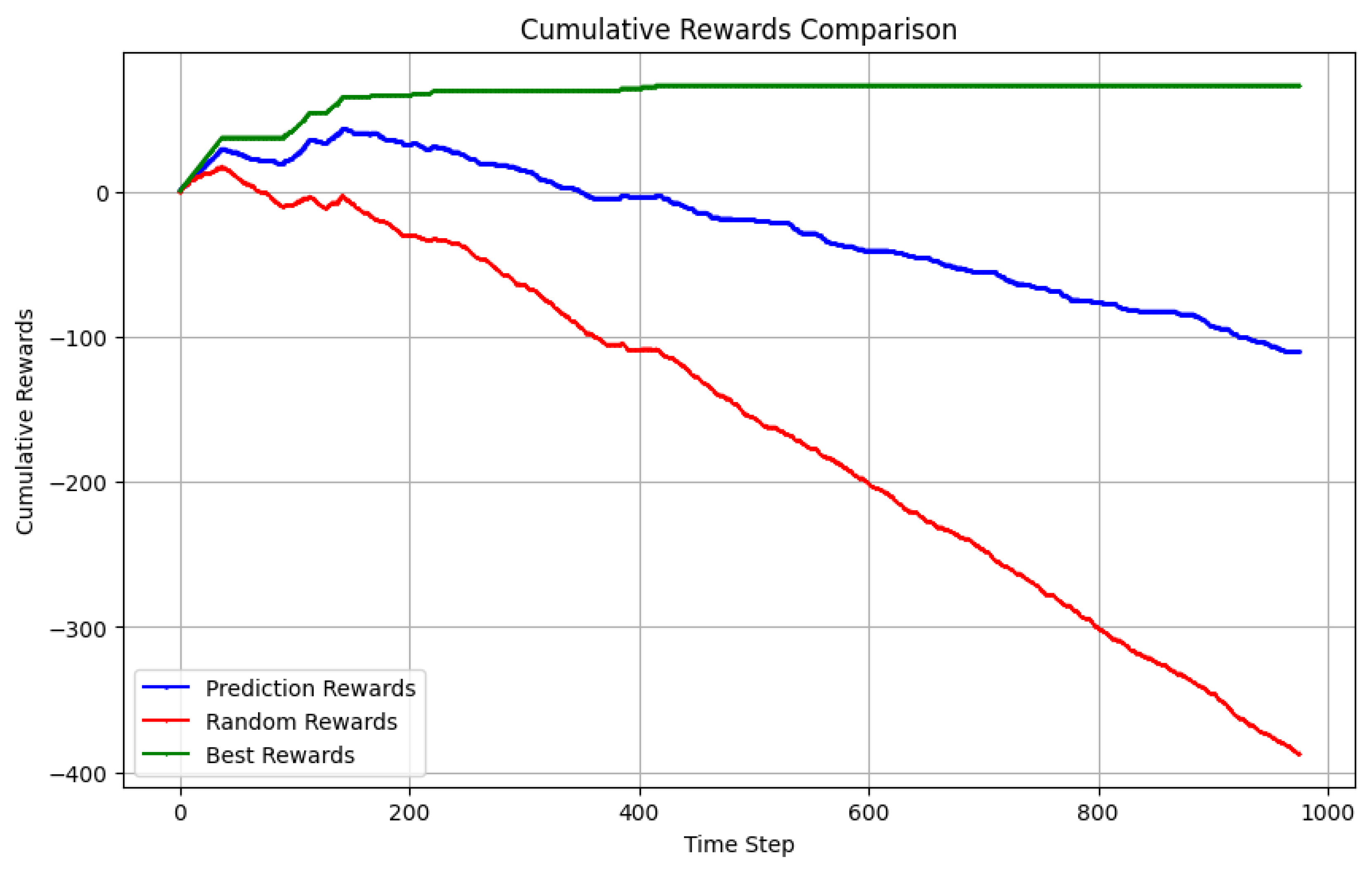
4.1. Underlying asset trend prediction
4.2. Options strategy evaluation
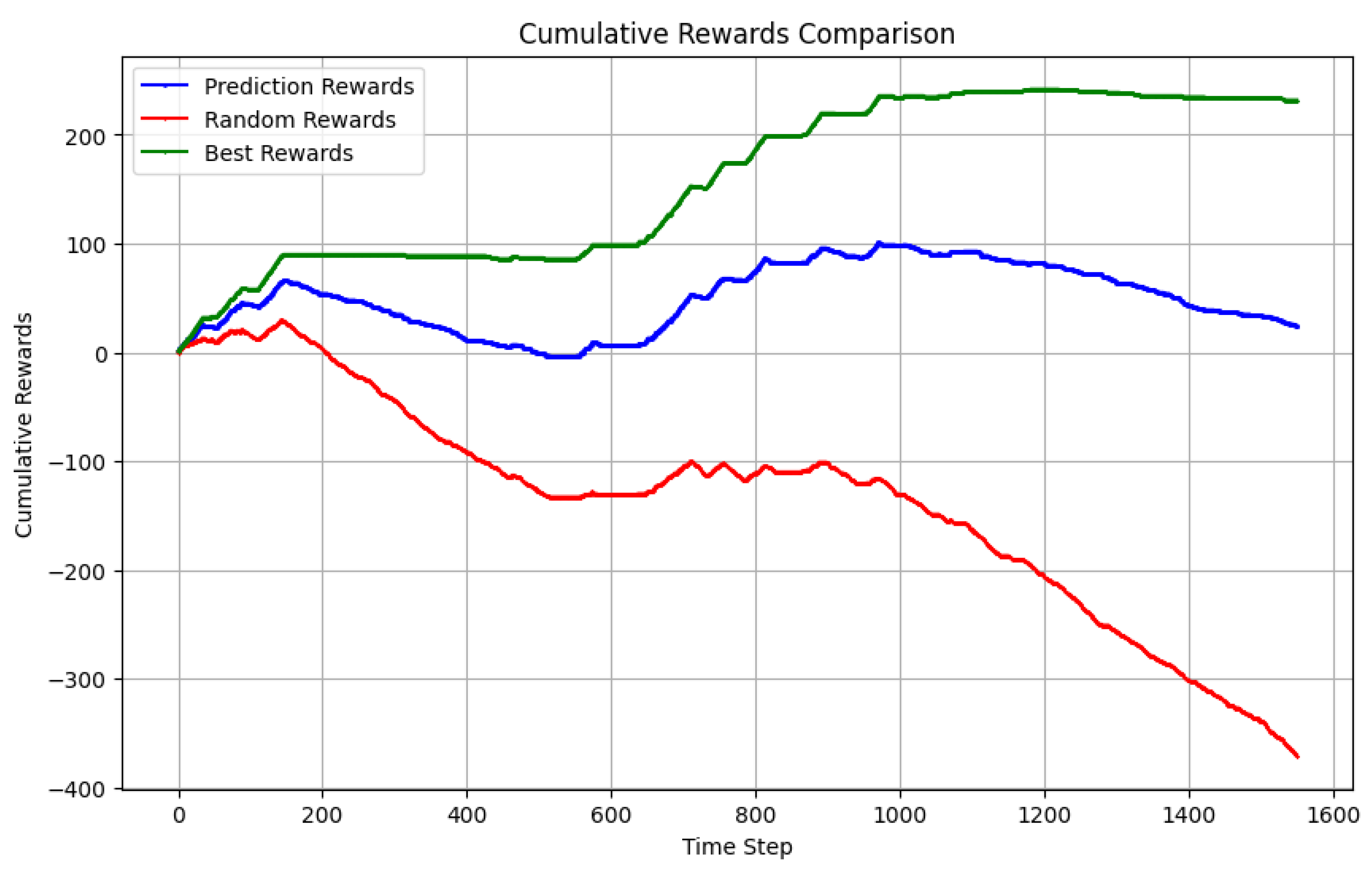
4.3. Backtesting
4.4. Option Selling with Predicted Trend
5. Discussion
6. Conclusion
Appendix
References
- P. Ciana, New Frontiers in Technical Analysis: Effective Tools and Strategies for Trading and Investing, 1st ed. Bloomberg Press, Sept.2011. [Online]. Available: https://learning.oreilly.com/library/view/new-frontiers-in/9781576603765/ (accessed Jul. 01, 2024).
- G. Cohen, Bible of options strategies, the: the definitive guide for practical trading strategies, 2nd ed. Pearson, 2005. pp.31,176,180. [Online]. Available: https://learning.oreilly.com/library/view/the-bible-of/9780133964431/ (accessed Jul. 03, 2024).
- V. Drakopoulou, "A Review of Fundamental and Technical Stock Analysis Techniques," Journal of Stock & Forex Trading, vol. 5, no. 1, Nov. 9, 2016. [Online]. Available: https://ssrn.com/abstract=3204667. (accessed Jul. 01, 2024).
- S. Ravichandiran, Hands-On Reinforcement Learning with Python. Packt Publishing, Jun. 2018. [Online]. Available: https://learning.oreilly.com/library/view/hands-on-reinforcement-learning/9781788836524/ (accessed Jul. 02, 2024).
- Y. Hilpisch, Artificial Intelligence in finance, 1st ed., O’Reilly Online Learning, Oct. 2020. [Online]. Available: https://learning.oreilly.com/library/view/artificial-intelligence-in/9781492055426/ (accessed Jul. 06, 2024).
- Joshi, B. Venkateswaran, and R. Bhattacharyya, “Options selling using machine learning,” Social Science Research Network, Apr. 2024. [Google Scholar] [CrossRef]
- Z. Kakushadze and J. A. Serur, “151 trading strategies”, Z. Kakushadze and J.A. Serur. 151 Trading Strategies. Cham, Switzerland: Palgrave Macmillan, an imprint of Springer Nature, 1st Edition (2018), XX, 480 pp. 17-39, 46, 40-60; ISBN 978-3-030-02791-9, Aug. 17, 2018. [Online]. Available: https://papers.ssrn.com/sol3/papers.cfm?abstract_id=3247865 (accessed Jul. 02, 2024).
- Li, W. Application of Machine Learning in Option Pricing: A Review. 2022 7th International Conference on Social Sciences and Economic Development (ICSSED 2022). LOCATION OF CONFERENCE, ChinaDATE OF CONFERENCE; pp. 209–214.
- Majidi, N.; Shamsi, M.; Marvasti, F. Algorithmic trading using continuous action space deep reinforcement learning. Expert Syst. Appl. 2023, 235. [Google Scholar] [CrossRef]
- McKeon, R. Empirical patterns of time value decay in options. China Finance Rev. Int. 2017, 7, 429–449. [Google Scholar] [CrossRef]
- V. Morris, B. Newman, A Guide To Investing With Options, 1st ed. Lightbulb Press, Feb. 2004.
- Naufal, G.R.; Wibowo, A. Time Series Forecasting Based on Deep Learning CNN-LSTM-GRU Model on Stock Prices. Int. J. Eng. Trends Technol. 2023, 71, 126–133. [Google Scholar] [CrossRef]
- Businessline, "Rules to Capture Time Decay," Jul. 24, 2022. [Online]. Available: www.proquest.com/newspapers/rules-capture-time-decay/docview/2693197982/se-2. [Accessed: Jul. 7, 2024].
- Businessline, "Trading Time Decay in Options," Nov. 6, 2022. [Online]. Available: www.proquest.com/newspapers/trading-time-decay-options/docview/2732145904/se-2. [Accessed: Jul. 7, 2024].
- Wang, X.; Li, J.; Li, J. A Deep Learning Based Numerical PDE Method for Option Pricing. Comput. Econ. 2022, 62, 149–164. [Google Scholar] [CrossRef]
- Wen, W.; Yuan, Y.; Yang, J. Reinforcement Learning for Options Trading. Appl. Sci. 2021, 11, 11208. [Google Scholar] [CrossRef]
- Wu, M.-E.; Syu, J.-H.; Chen, C.-M. Kelly-Based Options Trading Strategies on Settlement Date via Supervised Learning Algorithms. Comput. Econ. 2022, 59, 1627–1644. [Google Scholar] [CrossRef]
- Xu, F.; Ma, J. Intelligent option portfolio model with perspective of shadow price and risk-free profit. Financial Innov. 2023, 9, 1–28. [Google Scholar] [CrossRef]
- E. F. Fama and K. R. French, "Production of U.S. Rm-Rf, SMB, and HML in the Fama-French Data Library," Chicago Booth Research Paper No. 23-22, Fama-Miller Working Paper, Dec. 18, 2023. [Online]. Available: https://ssrn.com/abstract=4629613. [CrossRef]
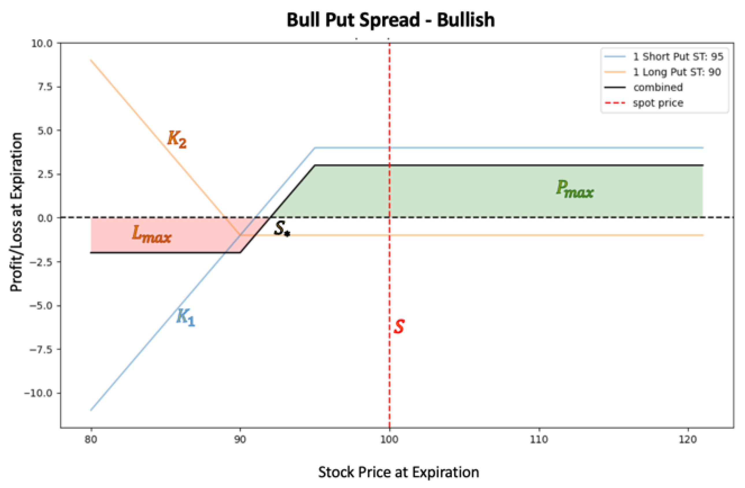


| Strategy | Equations | Definitions |
|---|---|---|
| Bull Put Spread | 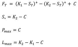 |
is the payoff at maturity T is the stock price at maturity T is the net credit received at t=0 is the break-even price is the maximum profit at maturity is the maximum loss at maturity |
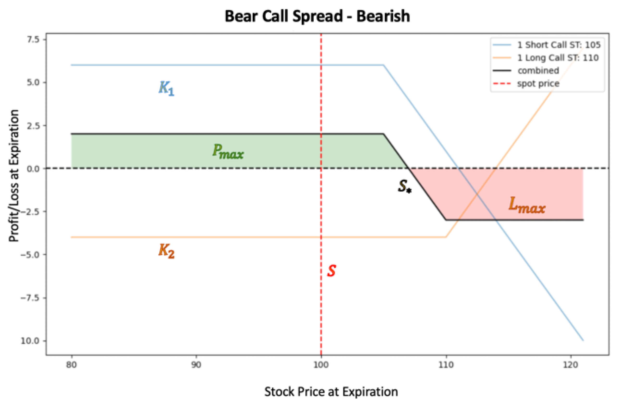
| Bear Call Spread | 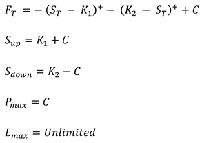 |
is the payoff at maturity T is the stock price at maturity T is the net credit received at t=0 is the break-even price is the maximum profit at maturity is the maximum loss at maturity |
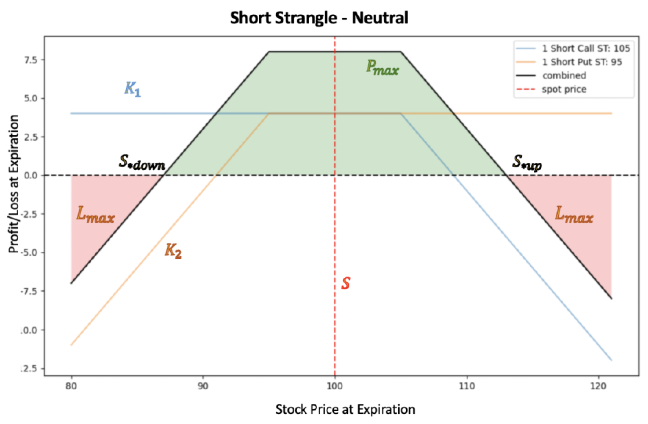
| Strangle | |
is the payoff at maturity T is the stock price at maturity T is the net credit received at t=0 is higher break-even is lower break-even is the maximum profit at maturity is the maximum loss at maturity |
| Data | From | To | Periodicity | Source |
|---|---|---|---|---|
| OHLCV | 2018-08-27 | 2023-12-14 | Daily | Yahoo Finance |
| Historical Options Chain | 2020-01-09 | 2023-10-31 | Daily (with monthly expiries) | OptionsDX |
| Future Options Chain | 2023-01-11 | 2023-12-31 | Daily (with monthly expiries) | Yahoo |
| Fama-French Factors | 2018-08-27 | 2023-12-14 | Daily | FF Research Data 5_Factors_2x3_daily |
| Bull Put Spread | Bear Call Spread | Short Strangle |
|---|---|---|
| HIGHER_STRIKE | HIGHER_STRIKE | HIGHER_STRIKE |
| LOWER_STRIKE | LOWER_STRIKE | LOWER_STRIKE |
| UNDERLYING_LAST | UNDERLYING_LAST | UNDERLYING_LAST |
| QUOTE_DATE | QUOTE_DATE | QUOTE_DATE |
| EXPIRY_DATE | EXPIRY_DATE | EXPIRY_DATE |
| SHORT_PUT_BID | SHORT_CALL_BID | SHORT_PUT_BID |
| SHORT_PUT_DELTA | SHORT_CALL_DELTA | SHORT_PUT_DELTA |
| LONG_PUT_ASK | LONG_CALL_ASK | SHORT_CALL_ASK |
| LONG_PUT_DELTA | LONG_CALL_DELTA | SHORT_CALL_DELTA |
| MAX_PROFIT | MAX_PROFIT | MAX_PROFIT |
| NET_DELTA | NET_DELTA | NET_DELTA |
| PROB_OF_EXPIRING_WORTHLESS | PROB_OF_EXPIRING_WORTHLESS | PROB_OF_EXPIRING_WORTHLESS |
| DTE | DTE | DTE |
| MAX_MARGIN | MAX_MARGIN | MAX_MARGIN |
| EXPECTED_RETURN_ON_MARGIN | EXPECTED_RETURN_ON_MARGIN | EXPECTED_RETURN_ON_MARGIN |
| Data | From | To | Model |
|---|---|---|---|
| Training/Validation | 2018-08-27 | 2023-05-22 | LSTM-CNN Hyperparameter Tuning and Training 80:20 |
| Testing | 2023-05-23 | 2023-11-15 | LSTM-CNN Price prediction |
| Prediction | 2023-11-16 | 2023-12-14 | Price Prediction 20 days |
| Parameter | Best Model | Search Space |
|---|---|---|
| LSTM units | 128 | min: 32, max: 128, step: 32, sampling: linear |
| Convolutional filters | 32 | min: 16, max: 64, step: 16, sampling: linear |
| Dense units | 128 | min: 64, max: 256, step: 64, sampling: linear |
| Learning rate | 0.00397 | min: 0.0001, max: 0.01, step: No, sampling: log. |
| Input LSTM leg | Long term data (11): AAPL OHLCV, EMA200, Fama-French 5 Factors | |
| Input CNN leg | Patterns (15): AAPL Technical indicators, VIX | |
| Output | 20 days prediction | |
| Target | Close price | |
| Validation loss | 0.003841 | |
| Data | From | To |
|---|---|---|
| Training | 2020-09-01 | 2023-05-22 |
| Testing | 2023-05-23 | 2023-10-31 |
| Prediction | 2023-11-01 | 2023-12-31 |
| Data | Value |
|---|---|
| Batch | 224 |
| Steps | 56 |
| Gamma (Discount Factor) | 0.930 |
| Learning Rate | |
| Entropy Coefficient | |
| Clip Range | 0.395 |
| Number of epochs | 3 |
| Lambda | 0.990 |
| Maximum Gradient Norm | 1.089 |
| Value Function Coefficient | 0.520 |
| Data | Value |
|---|---|
| Batch | 240 |
| Steps | 60 |
| Gamma (Discount Factor) | 0.880 |
| Learning Rate | |
| Entropy Coefficient | |
| Clip Range | 0.361 |
| Number of epochs | 13 |
| Lambda | 0.865 |
| Maximum Gradient Norm | 2.527 |
| Value Function Coefficient | 0.181 |
| Data | Value |
|---|---|
| Batch | 208 |
| Steps | 52 |
| Gamma (Discount Factor) | 0.893 |
| Learning Rate | |
| Entropy Coefficient | |
| Clip Range | 0.188 |
| Number of epochs | 3 |
| Lambda | 0.880 |
| Maximum Gradient Norm | 2.267 |
| Value Function Coefficient | 0.485 |
| Strategy | Bull Put Spread | Bear Call Spread | Short Strangle | |||
|---|---|---|---|---|---|---|
| PPO Model | Base | Best | Base | Best | Base | Best |
| Total Margin (USD) | 66678 | 80825 | 1023 | 1023 | 199330 | 232930 |
| Total Profit (USD) | 6341.9 | 8062 | 134 | 134 | 12563 | 15394 |
| Total Trades | 209 | 255 | 3 | 3 | 63 | 74 |
| Successful Trades | 149 | 181 | 2 | 2 | 51 | 61 |
| Unsuccessful Trades | 60 | 74 | 1 | 1 | 12 | 13 |
| Strategy | Bull Put Spread |
|---|---|
| PPO Model | Best/Trade |
| Total Margin (USD) | 1953 |
| Total Profit (USD) | 797 |
| Total Trades | 7 |
| Successful Trades | 7 |
| Unsuccessful Trades | 0 |
Disclaimer/Publisher’s Note: The statements, opinions and data contained in all publications are solely those of the individual author(s) and contributor(s) and not of MDPI and/or the editor(s). MDPI and/or the editor(s) disclaim responsibility for any injury to people or property resulting from any ideas, methods, instructions or products referred to in the content. |
© 2025 by the authors. Licensee MDPI, Basel, Switzerland. This article is an open access article distributed under the terms and conditions of the Creative Commons Attribution (CC BY) license (https://creativecommons.org/licenses/by/4.0/).


