
Submitted:
20 December 2024
Posted:
23 December 2024
You are already at the latest version
Abstract
Supersonic vacuum generators, or ejectors, operate pneumatically to extract air from a tank for industrial applications. A key performance metric for ejectors is the Total Evacuation Time (TET), which measures the time required to reach minimum pressure. This research predicts TET using analytical models that rely on two key metrics: the characteristic curve, relating absorbed flow rate to the working pressure, and the polytropic curve, which describes the evolution of the polytropic coefficient across working pressures. Accurately capturing both curves for subsequent fitting to polynomial curves, is crucial for forecasting TET. Several experimental setups were employed to capture the curves, each of which refined the data and improved the quality of the polynomial fits and coefficients. Multiple setups were necessary to pinpoint the break point, from supersonic to subsonic operation mode, which is a critical factor that affects the characteristic curve and the TET. Furthermore, the research shows an improvement in the TET forecasts for each setup with deviations between experimental and predicted TET ranging from 7.6 % (14.5 s}) to a 1.4 % (2.6 s) in the most precise setup. Once the models were validated, a new ejector obtained through CFD simulations, extracted from an authors previous article, was tested. It revealed a 4 % improvement (8 s}) in the TET. These results highlight the importance of the mathematical models developed, which can be used in the future to compare ejectors and reduce the need for experimental data.
Keywords:
Experimental study
; Vacuum generator
; One-stage Supersonic ejector
; Characteristic curve
; Polytropic curve
; Evacuation time
1. Introduction
Supersonic vacuum generators, also known as vacuum ejectors or simply ejectors, are essential components in modern industrial automation systems [1]. A key performance metric for ejectors is the Total Evacuation Time (TET), which measures the time required to reach the minimum pressure, with shorter times preferred for evacuating a reference volume. This research focuses on analytical prediction of the TET, referred to as the Predicted Total Evacuation Time (PTET). Other key design metrics for ejectors include the characteristic curve , which relates the change of the absorbed flow rate (or secondary flow) to the working pressure [2], and the polytropic coefficient evolution curve , which relates the change of the polytropic coefficient to the working pressures. These metrics provide the basis for comparing ejectors and improving their performance. Since TET directly influences the efficiency and suitability of ejectors for various applications [3], accurately predicting PTET relies on precisely capturing both the characteristic curve and the polytropic curve . Precise experimentation setups allows to evaluate the variation of flow rate and the polytropic coefficient across different working pressures, leading to the development of the and curve.
This paper is organised as follows. Section 2 explains the operation principle for the ejectors and reviews the existing literature regarding experiments of ejectors performance. Section 3 outlines the experimental setups for data collection, shows the polynomial formulas used, and introduces the analytical mathematical model to forecast the evacuation time. Section 4 presents the experimental findings and compares them with the results of the mathematical model. Finally, Section 5 discusses the results, while Section 6 draws the conclusions of the study.
2. Operating Principles and Background of Ejectors
The operational performance of the ejector is primarily determined by its internal geometry. Using the Venturi principle, the ejectors use compressed air as the primary flow to create the secondary flow rate of air from the secondary inlet. When the secondary inlet gets connected to a closed tank, this process empties the tank, enabling the use of the generated vacuum for automation applications, such as the use of vacuum cups for moving objects. This process is captured with the curve. The minimum pressure is achieved when the ejector can no longer absorb air, causing the secondary inlet flow rate to drop to zero. Figure 1 shows the internal configuration of an ejector and the two working flow rates. Thermodynamically, the emptying of an air-filled tank has a polytropic impact, shown by the polytropic curve.
Plenty of literature has been written on experiments with supersonic nozzles. As part of geometric and operating parameter studies, Hedge [4] explored nozzle positioning for industrial supersonic ejectors, and Lamberts [5] validated Fabri-choking’s significance. Ramesh [6,7] optimized the efficiency of ejector refrigeration through geometric adjustments and integration of renewable energy, while Chen [8] analysed the pressure distribution in a two-stage multi-nozzle system. Garcia del Valle [9,10] studied R-134a ejector refrigeration systems, focusing on pressure recovery and mixing chamber designs. His experiments revealed a transition point where the secondary flow rate changes from supersonic to subsonic. Mazzelli [11] validated a CFD model for a supersonic air ejector, highlighting accurate turbulence modelling, while Jafarian [12] validated a numerical model improving suction flow rate and reducing incidence time in vacuum ejectors, both with experimentation, highlighting the importance of the TET. Others have focused their research on the optimisation and performance enhancement of ejectors, Alimohammadi [13] developed a validated optimization method for a supersonic ejector compressor used in vehicle waste heat recovery, while Zhang [14] explored the optimal position of the nozzle for subsonic ejectors through experimental and CFD analysis. Ameur et al. [15,16,17] provided extensive experimental results on two-phase R134a ejectors, highlighting that a convergent-divergent nozzle improves the entrainment ratio, while a convergent nozzle is less affected by subcooling variations. Experimenting with the adjustable multistage ejector, Chen et al. [18,19] found that two-stage ejector refrigeration systems driven by dual heat sources offer better refrigerating effects at condensation temperatures below 21. C compared to single stage systems. Kun [20] examined adjustable ejectors with axial spindles, showing that a smaller nozzle throat area increases the entrainment ratio but reduces the discharge pressure, suggesting more economical design possibilities. In Noise Reduction and Mixing Characteristics, Zaman [21] found that tabs and ejectors reduced noise but less than expected due to flow instability. Karthick [22] showed experimentally that the entrainment ratio in a rectangular supersonic ejector varies with the expansion mode and Mach number ratio.
As noted above, the polytropic coefficient is crucial in the process of discharging an air-filled tank, as highlighted in authors previous studies [3]. Thorncroft [23] developed a model to predict the pressure and temperature of the tank during charging and discharging, noting that the polytropic exponent varies with the conditions and time.
Although the literature agrees on the importance of the TET, no literature was found regarding the PTET through analytical models.
3. Materials and method
3.1. Analytic Equation
As stated in the Section 1, TET is a key metric for comparing the performance of vacuum ejectors. For the PTET, it is necessary to establish a relationship between the decrease in pressure with time (), the and the curves. Both curves depend on the pressure inside the tank [3]. The relation can be found by taking the derivative of the definition of density and reorganising terms:
The reorganization of the polytropic equation we obtain:
where the k is a generic constant. Combining Eq. (2) with the perfect gas equation yields:
Combining Eq. (1) and Eq. (2) makes:
Introducing Eq. (3) in Eq. (4), derives into the relation between the differential pressure and time, the polytropic curve, and the characteristic curve, :
where the volume (V) in this work is considered constant value of 0.. The temperature (T) can be approximated as constant as 298K and r is the constant of the air gas equal to 287J kg K.
3.2. Parameterization of the Fitting Curves
The characteristic curve, , is the relationship between the secondary flow and the working pressure of an ejector. This relation is linear, according to [1,3], and it is parameterized by the first-order polynomial equation:
where a is the offset and b is the multiplier.
The improved experimental setups refined the data and exposed the transition or break point (bP), as exposed by [3,9,10], where is the value of the bP’s pressure and is the bP’s flow rate. Beyond bP, the behaviour of the secondary flow changes and the parameters of the linear equation adjust, captured piece-wise:
The polytropic curve, , relates the polytropic coefficient evolution to the ejector’s working pressure or secondary pressure. Authors past work[3] showed that near atmospheric pressure, the polytropic coefficient is adiabatic (), and near the minimum working pressure of the ejector it is isothermal (). Depending on the data trend, the fitting curve is first-order polynomial:
Or a second-order polynomial, its terms appear in blue.
3.3. Experimental Data Acquisition Setups
Two types of experiments are required to capture the characteristic and polytropic curves. Both use the same setup with different configurations. Figure 2 shows the experimental schematic and Figure 3 shows the laboratory setup used to obtain data for fitting to the curves explained in Section 3.2.
Valve V1 starts the experiment. The flow meter DP, a differential manometer, measures the primary flow rate and has the same error along the setups of kg s (1%). LRN, a long radius nozzle, measures the secondary flow rate of the secondary inlet. They were both constructed as instructed in ISO 5167-2:2022 [24]. Pressure sensor P1 measures the primary inlet pressure and has the same error along the setups of 0.0175bar (0.25%). A vacuum pressure sensor P2 measures the tank pressure which ranges from 1 bar(a) to 0.2bar(a). The first experiment captures the characteristic curve. The two-way flow restrictor valve V2 is closed incrementally and flow rates are measured with the flow meter, LRN. The second experiment captures the evolution of secondary pressure over time with the valve V2 closed preventing atmospheric air from entering.
In this study, two different sensor approaches are used for the experiments, and up to four setups are used to capture the required data, as explained in Section 3.2. The first approach is used in the setups 1, 2 and 3. It uses hydrostatic liquid column manometer sensors. The second approach was only used in the setup 4. It uses electronic WIKA transducers (A-10) connected to a Keysight DAQ970A/DAQ973A, a Data Acquisition System (DAS), shown in Figure 4.
For the first approach, the data was taken manually which had an uncomputed impact on the exact error, and the chronometer, not shown in Figure 2, is used to capture time. The chronometer is already incorporated into the DAS system, the setup 4. P2 is a heavier density fluid manometer. LRN uses a manometer to capture the flow rate and its design was different along the setups as detailed in the list.
- Setup 1: Used a long-radius nozzle of 10.5mm, shown in Figure 5. Water is used.
- Setup 2: Used a long-radius nozzle of 5.15mm, shown in Figure 5. Water is used.
- Setup 3: The same as in setup 2. Alcohol is used, with 0.7918.
- Setup 4: WIKA A-10 transducters sensors are used for the P1, LRN and P2. All are connected to the DAS as shown in Figure 4. LRN used a long-radius nozzle of 10.5mm.
Table 1 outlines the errors introduced per setup and sensor devices. The implementation of the multiplexer enabled simultaneous data capture across multiple instances, resulting in greater accuracy. However, quantifying the exact improvement remains a challenge. Although the electronic device of the WIKA transducer provided slightly less precision, it facilitated capture of data points simultaneously, enhancing overall data acquisition efficiency.
3.4. Mathematical Models to Predict Evacuation Time
Evacuation time is a key characteristic in comparing the performance of the vacuum ejector. It can be predicted using Eq.( 5), with the fitted experimental curve formula, explained in Section 3.2, for and . The mathematical model to forecast analytically the evacuation time, and the PTET, for the setups 1;2 is given by:
A piece-wise integration is required due to the regime change of , when the bP is evident, used for setup 3:
Finally, to predict the evacuation time for setup 4;5:
These integrals have been solved using the python environment quad, from the library scipy.integrate, that provides an interface to the library QUADPACK [25].
3.5. Testing Optimized Vacuum Ejector
In a previous study [2], the authors used CFD simulations to optimize the performance of a new ejector by changing its internal geometry. The parameters for this new design, referred to as setup 5, are and d (discussed in Section 3.2) and they are shown in Table 2. To validate the optimization, a PTET is forecasted and compared with the experimental TET. The analytical models developed in this study were applied, once validated, to determine the PTET.
To predict the evacuation time for the setup 5, the polytropic curve from the setup 4 were used due to the shared similarity of the characteristic curves.
4. Results
4.1. Experimental Results
As explained in Section 3.4, two types of experiments were conducted to collect the data. The first was used to obtain the characteristic curve , while the second was used to obtain the polytropic curve . Multiple setups were used to gradually improve the quality of the data, as explained in Section 3.3. These data were used to determine the fitting polynomial coefficients of and , both of which depend on the secondary pressure.
Figure 6 shows the refinement of the data used to capture the characteristic curve of , by setups 1;2;3. Setup 2 uses the data obtained in the setup 1 (in blue) and added the new captured data (in red). The same procedure for setup 3, which used the data captured by setup 1;2 (in blue) and added the new data (in red). The setup 3, described in Section 2, shows the evidence of the bP and was used in the piece-wise fitting equation.
Figure 7 shows the polytropic curve , and the corresponding fitting equations for each setup. The curve transitions from approximately 1.4 (adiabatic behaviour) at the start of evacuation (secondary pressure around 1bar) towards approximately 1 (isothermal behaviour), as outlined in [3]. The data captured by the setups 1;2;3 does not show a second-order polynomial trend.
Figure 8 shows on the left the characteristic curve captured with the setup 4. In the same graph it is compared the setup 4 and setup 5, taken from [2]. The data is presented along with its fitting curves, its equations, and the pressure break point. On the right there is the polytropic curve captured with setup 4 and its fitting curve. Capturing this curve using setup 4 shows a perfect second-order polynomial trend.
Table 3 shows the progression of the coefficients for the characteristic curve : a, b, and, if used, c and d as a piece-wise curve. The coefficients for the polytropic curve use the parameters e, f, and, if used, g. The n_exp1 shows the number of data used to obtain the coefficients of the experiment type 1.
4.2. Results on the Prediction of the Evacuation Time
The TET is a key metric for vacuum ejectors. Accurate PTET, as discussed in Section 3.4, relies on precise data capture to fit the polynomial coefficients of the characteristic and polytropic curves (Section 3.2). Table 4 displays the predicted and experimental evacuation times to reach the ejector minimum pressure from atmospheric pressure.
Figure 9 compares the deviation of predicted and experimental evacuation time for setups 1;2;3;4. The errors between PTET and experimental values are as follows: setup 1 has the highest error with a deviation of 14.5s (7.6%), setup 2 shows an error of 10.2s (5.3%), setup 3 has an error of -5.5s (2.9%), and setup 4 has the smallest error of 2.6s (1.4%), closely matching the experimental TET.
Setup 5 characteristic curve coefficients are given in Section 3.5. The polytropic curve obtained with setup 4 was used due to characteristic curve similarity. Figure 10 shows the predicted evacuation time for setup 4;5. The right graph zooms in on the end of the evacuation time. As anticipated in [2], the minimum pressure of setup 5 is lower than the tested with the setups 1;2;3;4, due to its optimized internal geometry.
Figure 11 illustrates the deviation between the experimental evacuation time and the predicted time from setup 5. At higher pressures, the predicted evacuation time exceeds the experimental values, with a maximum difference of 2s at 0.5bar(a). However, at lower pressures, setup 5 demonstrates improved performance by reducing the PTET by 8.1s (4%) compared to the experimental TET. This data is further corroborated in Table 4.
5. Discussion
The aim of this research was to anallytically predict the TET by creation mathematical models and using the characteristic and polytropic curves. The fitting of experimental data to polynomial curves is employed as a method for analytically predicting TET, as explained in Section 3.4. The R-squared values, which reflect the accuracy of the fit, are directly related to the refinement of the polynomial coefficients. Figure 6 presents the R-squared values for setups 1;2;3. Setup 1, despite having less data, shows a strong fit with an R-squared value rounded to 0.99805. In contrast, setup 2, which includes more data but has an ambiguous bP, displays greater variation and is the least consistent, with a rounded R-squared of 0.99794. Setup 3, where the bP is evident, demonstrates a better fit, yielding a rounded R-squared of 0.99876. Setup 4 achieves the highest data precision, as shown in Figure 8, where the R-squared value is rounded to 1.0, indicating an almost perfect fit. Table 3 presents the refinement of the polynomial coefficients and the appearance of the bP in setups 3;4. Table 4 highlights the significance of the polynomial coefficients and R-squared values, showing deviations in the PTET ranging from 7.6% to 1.4%. Incorporation of bP into and in the mathematical model has a significant impact on the PTET by almost halving it: in setup 2 the PTET against experimental TET deviation is 5.3% whereas in setup 3 is 2.9%.
Polytropic curve data from the setups 1;2;3 were fitted to a first-order polynomial due to the absence of a second-order trend (see Figure 7). In contrast, the setup 4 exhibited a second-order polynomial trend in its polytropic data (see Figure 8)), which contributed to a better fit. The second-order polynomial trend has a clear impact on PTET, as shown in Figure 9. In setup 3, the deviation between PTET and experimental TET is 2.9%, whereas in setup 4 halves this deviation to 1.4%. The PTET deviation of 1.4% (2.6s in absolute terms) demonstrates that the model successfully matches the TET, confirming its validity.
After model validation, a new optimized ejector, setup 5, was tested using data from an author’s previous work [2]. Figure 10 shows a setup 5 being the best with an overall performance improvement by reducing the minimum secondary pressure achieved and lowering the PTET by 4% (8s). The curve coefficients obtained in setup 4 are used to calculate the PTET for the setup 5, due to the similarity of . Figure 11 indicates that while PTET is lower, evacuation time is higher at mid-range working pressures, peaking at 2s at 0.5bar (a). Nonetheless, this is not a significant issue as the main objective of this research is to improve PTET relative to experimental TET.
Finally, the PTET of the experimental setup 4 shows a deviation error of 1.4% and the tested setup 5 showed an increase of performance about 4%. This difference exceeds the experimental error of1.4%, indicating its significance. These results highlight the importance of the mathematical models developed, which can be used in the future to compare ejectors and reduce the need for experimental data.
6. Conclusions
In this research, the Total Evacuation Time (TET), which measures how quickly an ejector can reach the lowest minimum pressure, is predicted by developing accurate analytical models that incorporate key ejector performance metrics, such as the characteristic curve and polytropic curve. Through refined experimental setups, it was succeeded in capturing data that improved the precision of these models, minimizing deviations between experimental and predicted results.
One findings of this work is the importance of the characteristic curve, which links the absorbed flow rate to the working pressure. The data and literature revealed a critical transition point, or breakpoint (bP), where the operation mode of the ejector shifts from supersonic to subsonic. This transition influences both the curve and the Predicted TET (PTET), and pinpointing this bP improved the accuracy of the mathematical models. The research demonstrated that with each refined setup, the PTET approached the actual experimental values more closely, reducing the error margin from 7.6% to just 1.4% in the most precise setup. The polytropic curve, which describes how the polytropic coefficient evolves as a function of working pressure, played an important role in forecasting the PTET. The experiments demonstrated that at higher pressures, the polytropic coefficient behaves adiabatically (1.4), while at lower pressures, it approaches isothermal conditions (1.0). Refinement of the experimental setup improved the fitting of data to the second-order polynomial trend, critically halving PTET error deviation from 2.91.4 in the most refined setup. The PTET error of 1.4% (2.6s in absolute terms) demonstrates that the analytical model successfully matches the TET, confirming its validity.
With the models validated, an optimized vacuum ejector design was tested, based on previous authors research via CFD simulations. This optimized ejector showed a 4% improvement in PTET (about 8s), exceeding the PTET error. The analytical models based on these curves, proved highly effective in reducing the dependency on additional experimental data, allowing for faster comparison and optimization of different ejector designs. This underscores the potential for combining experimental data with simulations to design more efficient industrial components, such as vacuum ejectors.
7. Future work
Pourmovahed [26] identified a relationship between the shape of the evacuation tank and the polytropic coefficient. He provided an experimental thermal time-constant correlation for gas-charged hydraulic accumulators, which enables an accurate prediction of thermodynamic losses and the history of gas pressure and temperature during compression or expansion. To validate Pourmovahed’s suggested thermal time-constant, future work will involve testing the ejector’s characteristic and polytropic curves with evacuation tanks of different shapes.
Another aspect of future work includes constructing the optimized ejector and testing it with the most refined setup configuration.
Acknowledgments
This research received external funding from Generalitat de Catalunya. Support of Industrial Doctorate (2018 DI 025) from Generalitat de Catalunya is acknowledged. Many thanks to laboratory technicians (J. Bonastre, Sr and J. Bonastre, Jr.), and the intern (J. Martinez) for their help.
References
- Macià, L.; Castilla, R.; Gamez-Montero, P.J.; Camacho, S.; Codina-Macia, E. Numerical Simulation of a Supersonic Ejector for Vacuum Generation with Explicit and Implicit Solver in Openfoam. Energies 2019. [Google Scholar] [CrossRef]
- Macia, L.; Castilla, R.; Gamez-Montero, P.J.; Raush, G. Multi-Factor Design for a Vacuum Ejector Improvement by In-Depth Analysis of Construction Parameters. Sustainability 2022, 14. [Google Scholar] [CrossRef]
- Macia, L.; Castilla, R.; Gámez, P.J. Simulation of ejector for vacuum generation. IOP Conference Series: Materials Science and Engineering 2019, 659, 012002. [Google Scholar] [CrossRef]
- Hegde, G.; Himakar, B.; Rao V, S.M.; , a. ; Kim, M.; Sohn, Y.J.; Lee, W.Y.; Falsafioon, M.; Aidoun, Z.; Poirier, M. A Numerical and Experimental Study of Ejector Internal Flow Structure and Geometry Modification for Maximized Performance. IOP Conference Series: Materials Science and Engineering 2017, 280, 012011. [Google Scholar] [CrossRef]
- Lamberts, O.; Chatelain, P.; Bartosiewicz, Y. Numerical and experimental evidence of the Fabri-choking in a supersonic ejector. International Journal of Heat and Fluid Flow 2018, 69, 194–209. [Google Scholar] [CrossRef]
- Ramesh, A.S.; Joseph Sekhar, S. Experimental Studies on the Effect of Suction Chamber Angle on the Entrainment of Passive Fluid in a Steam Ejector. Journal of Fluids Engineering 2017, 140. [Google Scholar] [CrossRef]
- Ramesh, A.S.; Sekhar, S.J. Experimental and numerical investigations on the effect of suction chamber angle and nozzle exit position of a steam-jet ejector. Energy 2018, 164, 1097–1113. [Google Scholar] [CrossRef]
- Chen, W.; Xue, K.; Chen, H.; Chong, D.; Yan, J. Experimental and Numerical Analysis on the Internal Flow of Supersonic Ejector Under Different Working Modes. Heat Transfer Engineering 2018, 39, 700–710. [Google Scholar] [CrossRef]
- García Del Valle, J.; Saíz Jabardo, J.M.; Castro Ruiz, F.; San José Alonso, J.F. An experimental investigation of a R-134a ejector refrigeration system. International Journal of Refrigeration 2014, 46, 105–113. [Google Scholar] [CrossRef]
- García del Valle, J.; Sierra-Pallares, J.; Garcia Carrascal, P.; Castro Ruiz, F. An experimental and computational study of the flow pattern in a refrigerant ejector. Validation of turbulence models and real-gas effects. Applied Thermal Engineering 2015, 89, 795–811. [Google Scholar] [CrossRef]
- Mazzelli, F.; Little, A.B.; Garimella, S.; Bartosiewicz, Y. Computational and experimental analysis of supersonic air ejector: Turbulence modeling and assessment of 3D effects. International Journal of Heat and Fluid Flow 2015, 56, 305–316. [Google Scholar] [CrossRef]
- Jafarian, A.; Azizi, M.; Forghani, P. Experimental and numerical investigation of transient phenomena in vacuum ejectors. Energy 2016, 102, 528–536. [Google Scholar] [CrossRef]
- Alimohammadi, S.; Persoons, T.; Murray, D.B.; Tehrani, M.S.; Farhanieh, B.; Koehler, J. A Validated Numerical-Experimental Design Methodology for a Movable Supersonic Ejector Compressor for Waste-Heat Recovery. Journal of Thermal Science and Engineering Applications 2013, 6. [Google Scholar] [CrossRef]
- Zhang, X.; Jin, S.; Huang, S.; Tian, G. Experimental and CFD analysis of nozzle position of subsonic ejector. Frontiers of Energy and Power Engineering in China 2009, 3, 167–174. [Google Scholar] [CrossRef]
- Ameur, K.; Aidoun, Z.; Ouzzane, M. Experimental performances of a two-phase R134a ejector. Experimental Thermal and Fluid Science 2018, 97, 12–20. [Google Scholar] [CrossRef]
- Ameur, K.; Aidoun, Z. Nozzle Displacement Effects on Two-Phase Ejector Performance: An Experimental Study. Journal of Applied Fluid Mechanics 2018, 11, 817–823. [Google Scholar] [CrossRef]
- Ameur, K.; Aidoun, Z.; Falsafioon, M. Experimental Performance of a Two-Phase Ejector: Nozzle Geometry and Subcooling Effects. inventions 2020. [Google Scholar] [CrossRef]
- Chen, G.; Zhang, R.; Zhu, D.; Chen, S.; Fang, L.; Hao, X. Experimental study on two-stage ejector refrigeration system driven by two heat sources. International Journal of Refrigeration 2017, 74, 295–303. [Google Scholar] [CrossRef]
- Chen, P. Experimental study on the entrainment performance and flow choking phenomenon of a two-stage multi-nozzle ejector. International Journal of Modern Physics B 2020, 34, 2040099. [Google Scholar] [CrossRef]
- Kun, Z.; Shengqiang, S.; Yong, Y.; Xingwang, T. Experimental Investigation of Adjustable Ejector Performance. Journal of Energy Engineering 2012, 138, 125–129. [Google Scholar] [CrossRef]
- Zaman, K.Q.; Castner, R.S.; Bridges, J.E.; Fagan, A.F.; Upadhyay, P. Experiments on Thrust, Flowfield and Noise of a Rectangular Mixer-Ejector Nozzle. In Proceedings of the AIAA Scitech 2020 Forum. American Institute of Aeronautics and Astronautics, AIAA SciTech Forum; 1 2020; p. 1. [Google Scholar] [CrossRef]
- Karthick, S.K.; Rao, S.M.V.; Jagadeesh, G.; Reddy, K.P.J. Parametric experimental studies on mixing characteristics within a low area ratio rectangular supersonic gaseous ejector. Physics of Fluids 2016, 28, 076101. [Google Scholar] [CrossRef]
- Thorncroft, G.; Patton, J.S.; Gordon, R. Modeling Compressible Air Flow in a Charging or Discharging Vessel and Assessment of Polytropic Exponent. Technical report, California Polytechnic State University, Honolulu, Hawaii, 2007. [CrossRef]
- ISO 5167-2:2022 - Measurement of fluid flow by means of pressure differential devices inserted in circular cross-section conduits running full — Part 2: Orifice plates, 2000.
- R. Piessens, E.D.D.K.; Überhuber., C.W. R. Piessens, E.D.D.K.; Überhuber., C.W. QUADPACK: a subroutine package for automatic integration, 1983. [Google Scholar]
- Pourmovahed, A.; Otis, D.R. An Experimental Thermal Time-Constant Correlation for Hydraulic Accumulators. Journal of Dynamic Systems, Measurement, and Control 1990, 112, 116–121. [Google Scholar] [CrossRef]
Figure 1.
Diagram of ejector geometry with internal geometry showing the two most important characteristics. The flow direction is from the left (main inlet) to the right (outlet).
Figure 1.
Diagram of ejector geometry with internal geometry showing the two most important characteristics. The flow direction is from the left (main inlet) to the right (outlet).
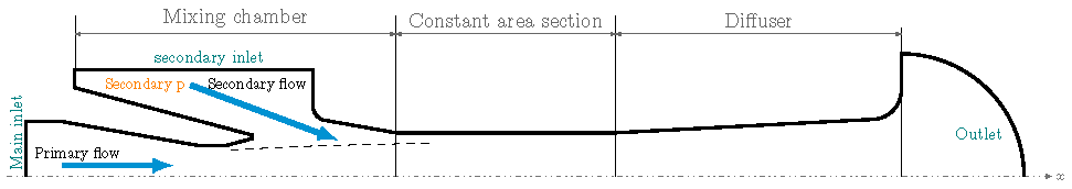
Figure 2.
Schematic of the setups used for experiments.
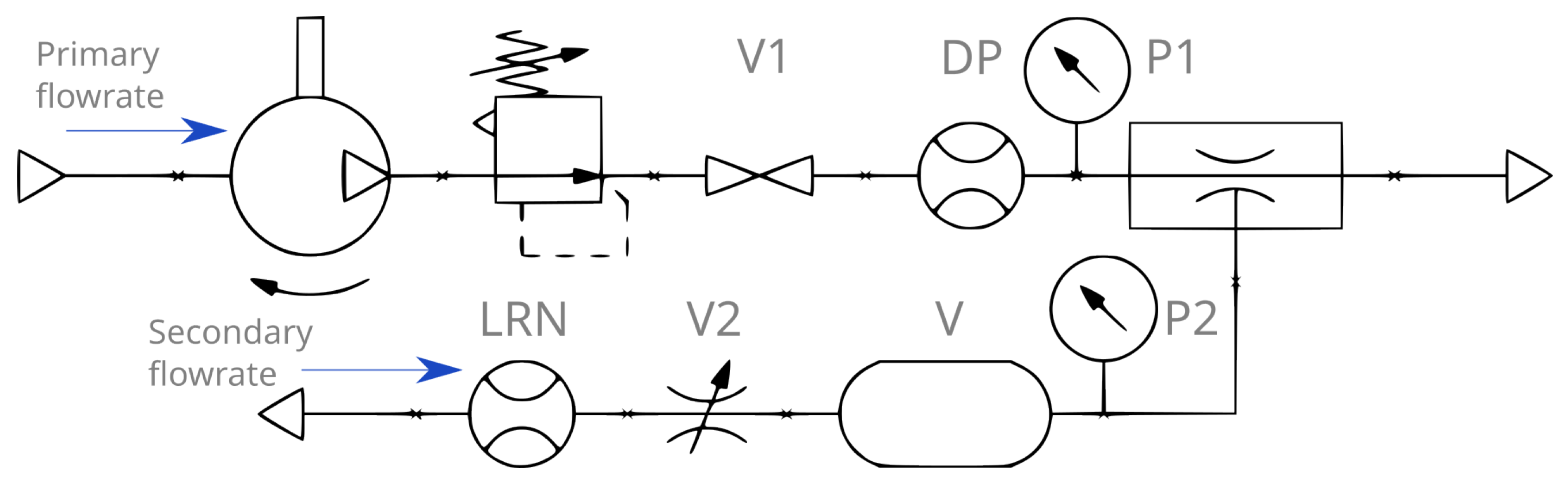
Figure 3.
Laboratory view of the experimental setup.
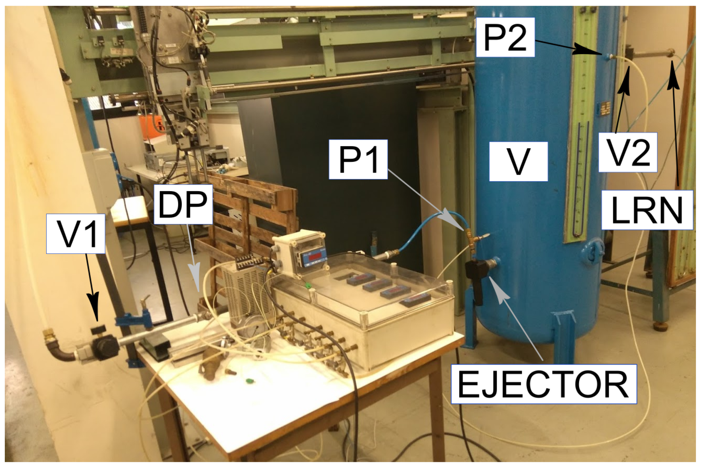
Figure 4.
Electronic circuit used to connect the WIKA sensors to the multiplexer.
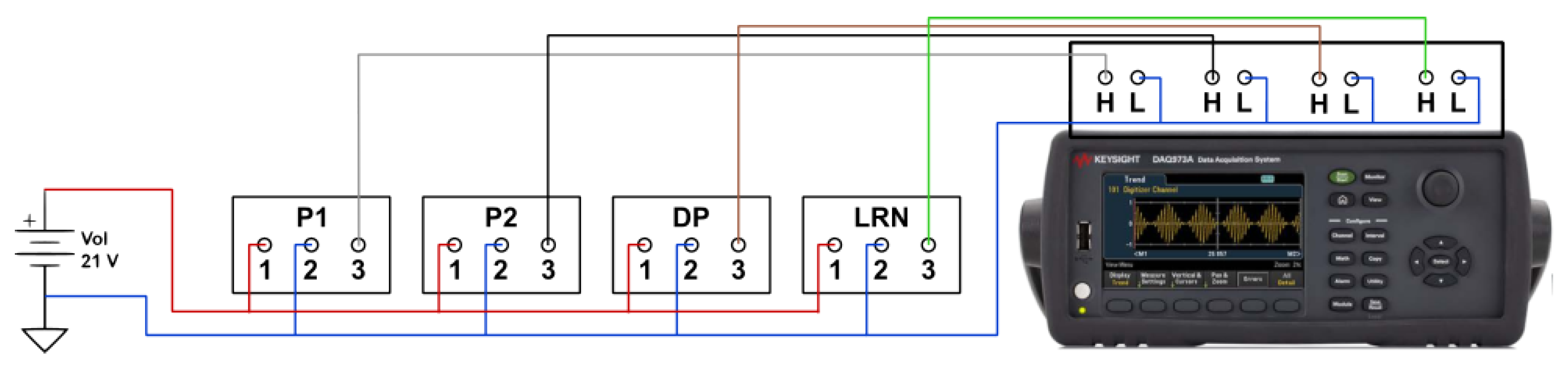
Figure 5.
Flowmeter LRN (a) used in setup 1;4 (b) used in setup 2;3 (c) Drawing of (b)
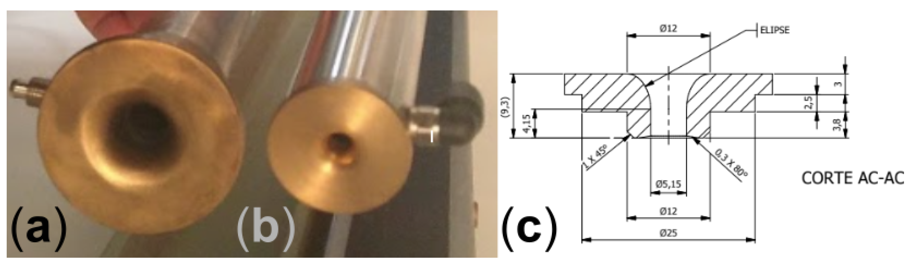
Figure 6.
Characteristic curve, , Setups 1;2;3. bP was introduced in setup 3.
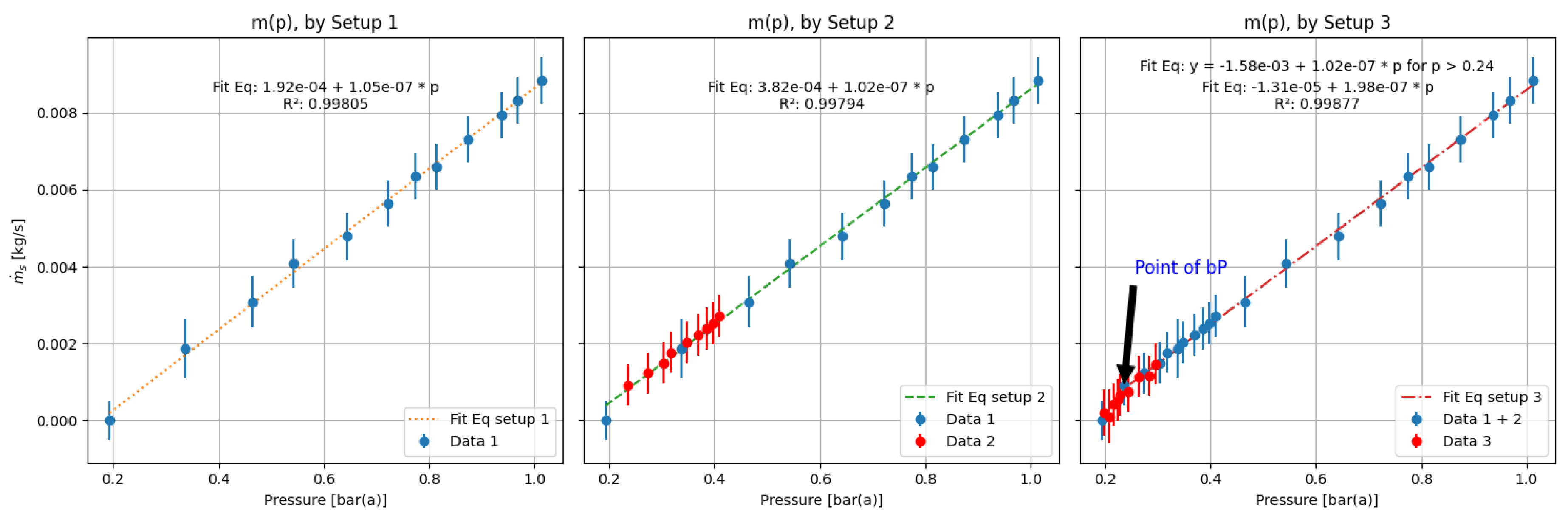
Figure 7.
Polytropic coefficient evolution, n(p), for setups 1;2;3.
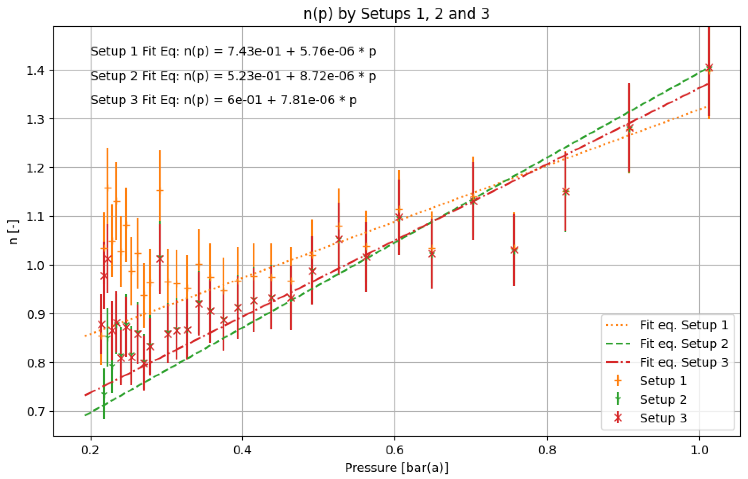
Figure 8.
Left: Characteristic curves, , captured by setup 4 and setup 5 [2]. Right: Polytropic curve, , captured by setup 4.
Figure 8.
Left: Characteristic curves, , captured by setup 4 and setup 5 [2]. Right: Polytropic curve, , captured by setup 4.
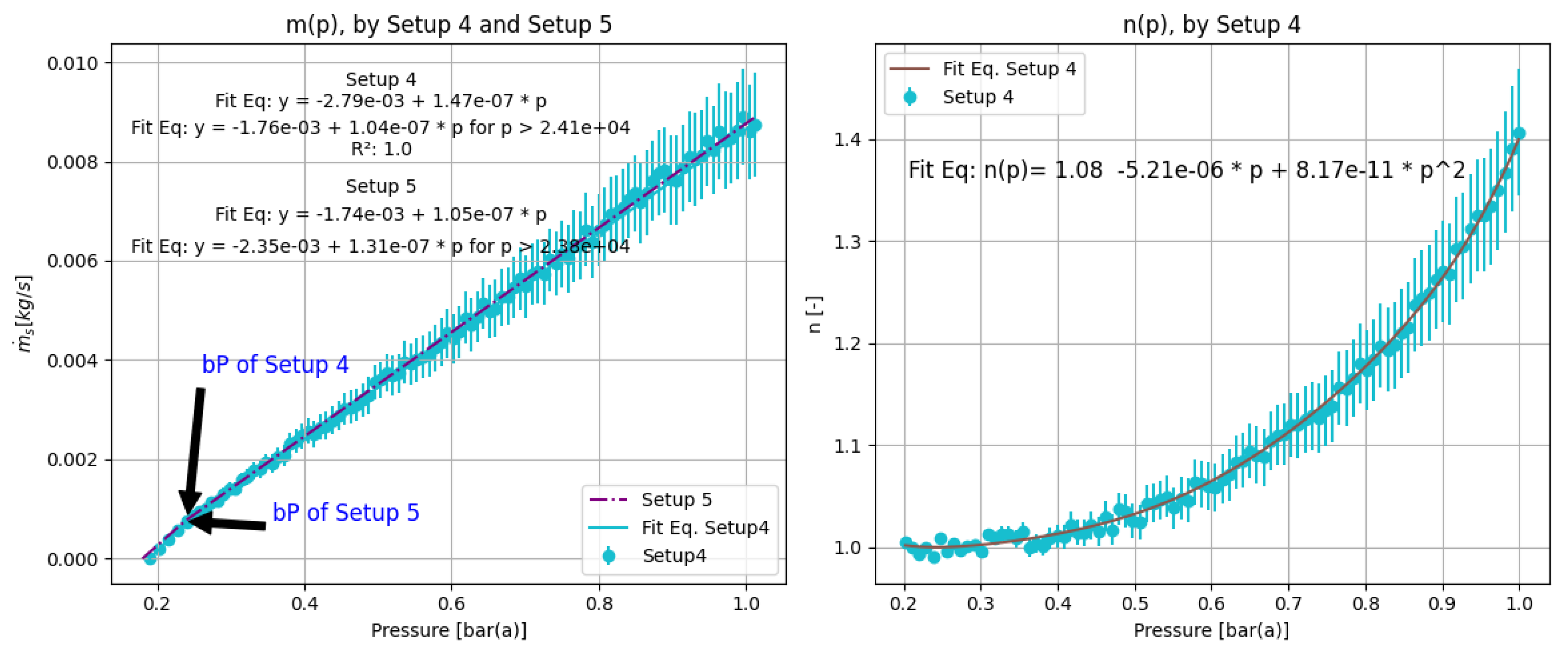
Figure 9.
Percentage deviation or error between experimental and predicted evacuation time for setups 1;2;3;4, for a tank with a volume of 0.5.
Figure 9.
Percentage deviation or error between experimental and predicted evacuation time for setups 1;2;3;4, for a tank with a volume of 0.5.
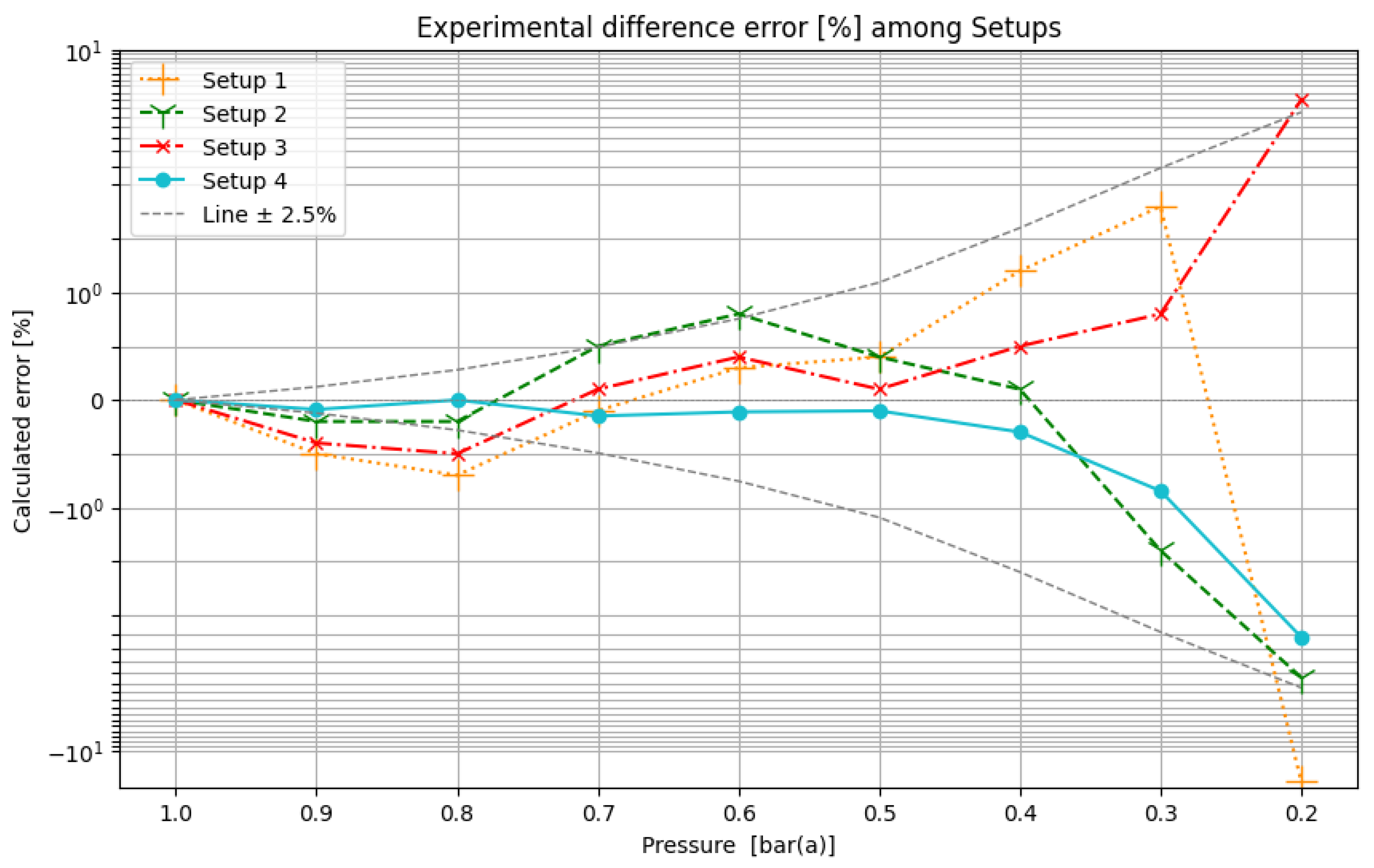
Figure 10.
Left: Predicted evacuation time graph for setups 4;5. Right: Zoomed-in view of the final evacuation stage. Setup 5 demonstrates better performance, achieving lower minimum pressure and shorter evacuation times.
Figure 10.
Left: Predicted evacuation time graph for setups 4;5. Right: Zoomed-in view of the final evacuation stage. Setup 5 demonstrates better performance, achieving lower minimum pressure and shorter evacuation times.
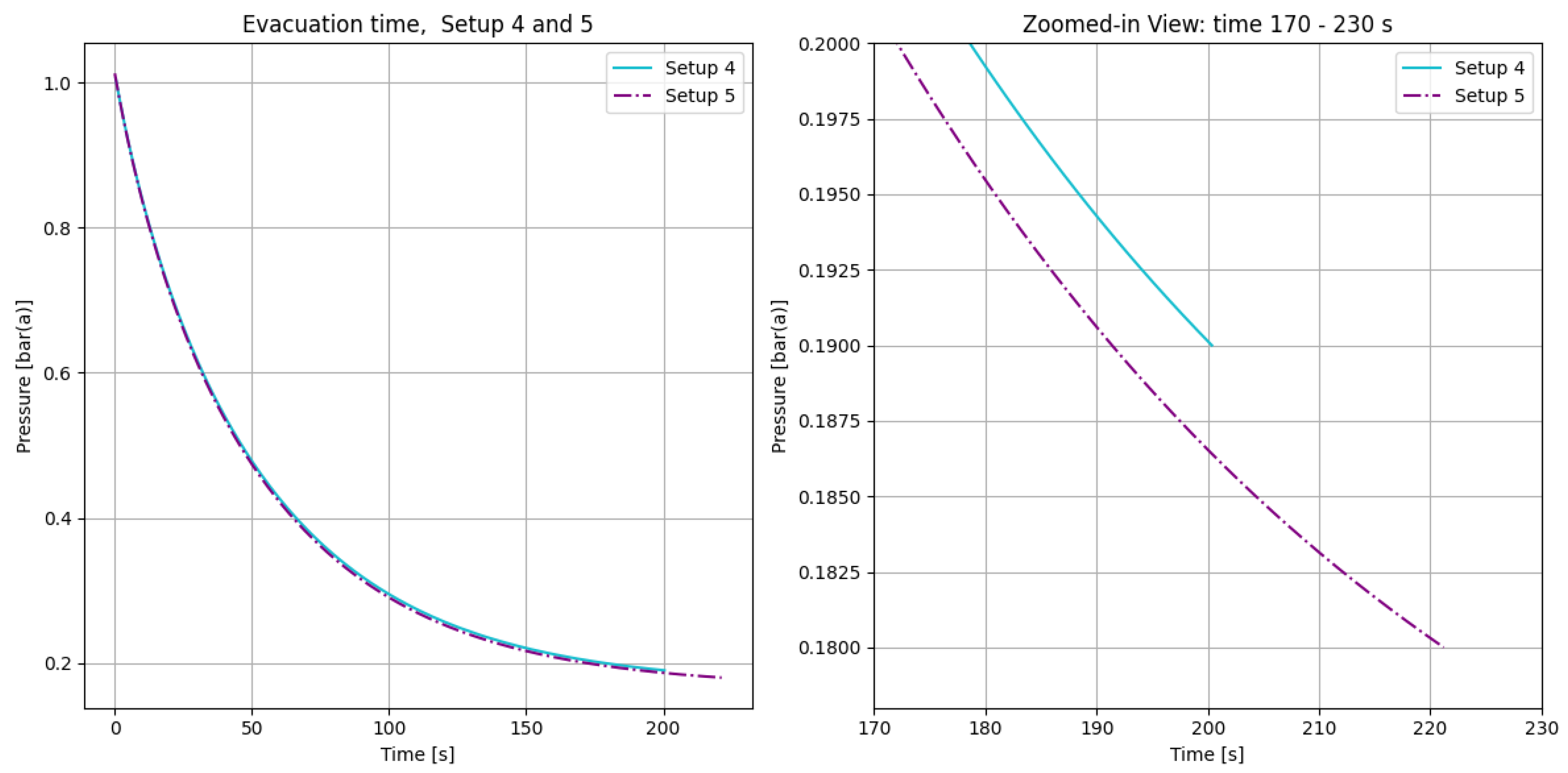
Figure 11.
Time deviation in seconds between experimental and predicted TET for setup 5, for a tank with a volume of 0.5.
Figure 11.
Time deviation in seconds between experimental and predicted TET for setup 5, for a tank with a volume of 0.5.
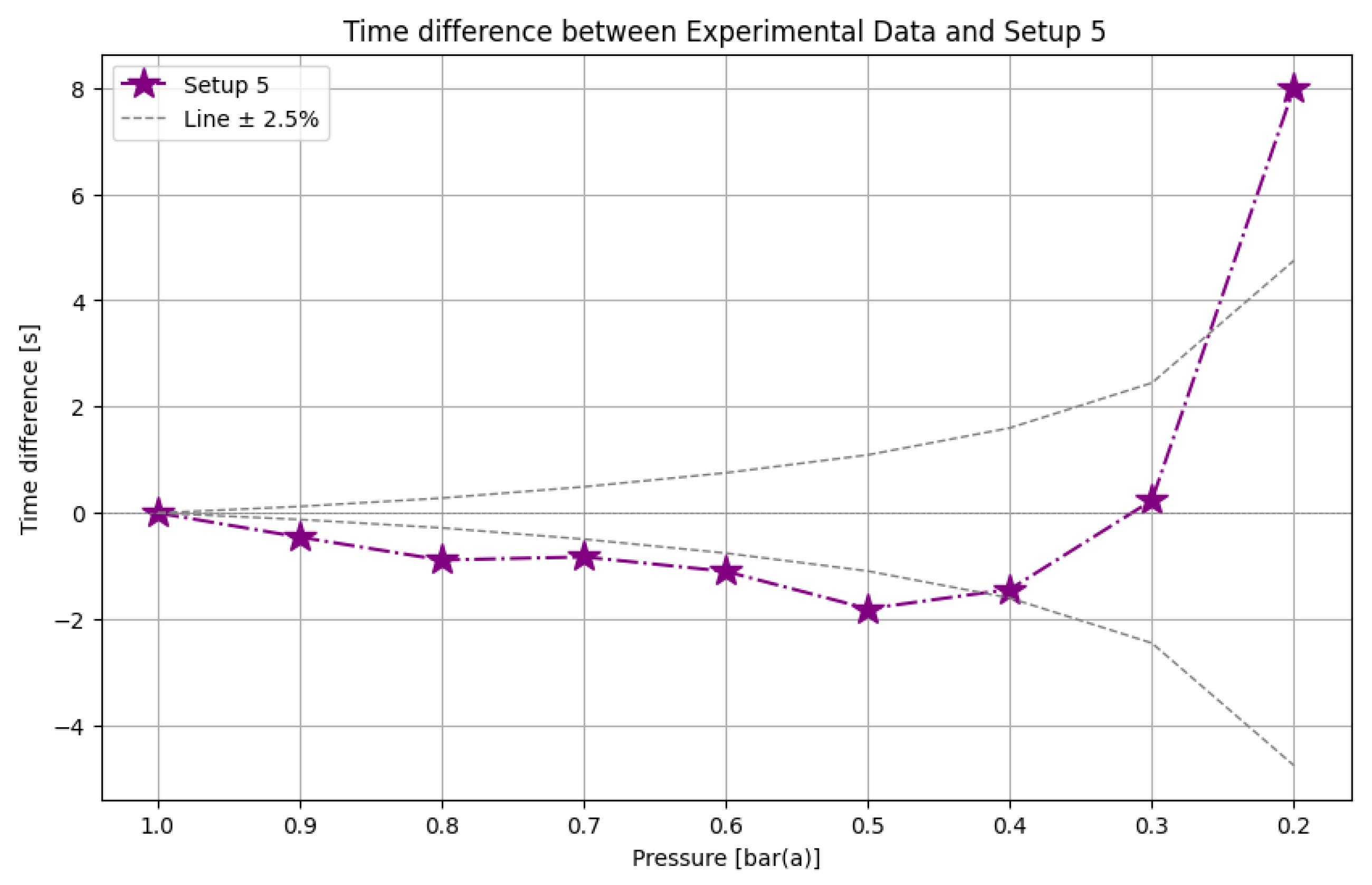

Table 1.
Error introduced per setup and sensor device
| Sensor | Unit | Setup 1 | Setup 2 | Setup 3 | Setup 4 |
|---|---|---|---|---|---|
| LRN | [kg s] | ||||
| LRN | [%] | 1.35 | 0.29 | 0.23 | 2.82 |
| P2 | [bar] | ||||
| P2 | [%] | 2.62 | 2.62 | 2.62 | 0.25 |
| Chronometer | [s] | 1 s | 1 s | 1 s | 0.01 s |
Table 2.
Coefficients used for the setup 5 [2]
Table 2.
Coefficients used for the setup 5 [2]
| Setup | a | b | c | d | ||
|---|---|---|---|---|---|---|
| 5 |
Table 3.
Summarized coefficients per setup
| Setup | a | b | c | d | e | f | g | n_exp1 | ||
|---|---|---|---|---|---|---|---|---|---|---|
| 1 | – | – | – | – | – | 12 | ||||
| 2 | – | – | – | – | – | 21 | ||||
| 3 | – | 30 | ||||||||
| 4 | 95 |
Table 4.
Temporal comparison at specific vacuum pressure levels.
|
Pressure [bar(a)] |
Experimental [s] | Setup 1 [s] | Setup 2 [s] | Setup 3 [s] | Setup 4 [s] | Setup 5 [s] |
|---|---|---|---|---|---|---|
| 1.0 | 0.0 | 0.0 | 0.0 | 0.0 | 0.0 | 0.0 |
| 0.9 | 4.9 | 5.4 | 5.1 | 5.3 | 5 | 5.4 |
| 0.8 | 11.2 | 11.9 | 11.4 | 11.7 | 11.2 | 12.1 |
| 0.7 | 19.7 | 19.8 | 19.2 | 19.6 | 19.8 | 20.5 |
| 0.6 | 30.2 | 29.9 | 29.4 | 29.8 | 30.3 | 31.3 |
| 0.5 | 43.7 | 43.3 | 43.3 | 43.6 | 43.8 | 45.5 |
| 0.4 | 64.0 | 62.8 | 63.9 | 63.5 | 64.3 | 65.4 |
| 0.3 | 97.9 | 96.1 | 99.3 | 97.1 | 98.7 | 97.7 |
| 0.2 | 190.0 | 204.5 | 200.2 | 184.5 | 192.6 | 181.9 |
Disclaimer/Publisher’s Note: The statements, opinions and data contained in all publications are solely those of the individual author(s) and contributor(s) and not of MDPI and/or the editor(s). MDPI and/or the editor(s) disclaim responsibility for any injury to people or property resulting from any ideas, methods, instructions or products referred to in the content. |
© 2024 by the authors. Licensee MDPI, Basel, Switzerland. This article is an open access article distributed under the terms and conditions of the Creative Commons Attribution (CC BY) license (http://creativecommons.org/licenses/by/4.0/).
Copyright: This open access article is published under a Creative Commons CC BY 4.0 license, which permit the free download, distribution, and reuse, provided that the author and preprint are cited in any reuse.


