
Submitted:
18 December 2024
Posted:
19 December 2024
You are already at the latest version
Abstract
This study examines how uncertainty and global risk affect financial markets in emerging economies, focusing on foreign investment, CDS spreads, exchange rates, and stock return volatility. Using over 8.6 million ticker-transaction observations and structural vector autoregression (VAR) models, the research finds that increases in Economic Policy Uncertainty (EPU) significantly reduce foreign net buys, more than global market volatility (VIX). While global volatility drives CDS spreads, these spreads influence exchange rates, causing currency depreciation. The findings highlight the interconnectedness of uncertainty, global risk, and market instability, offering insights for managing risks in opaque markets and improving financial stability.
Keywords:
Global risk
; uncertainty
; volatility
; opacity
; foreign investors
; VAR
; BSADF test
1. Introduction
Uncertainty has long been a defining characteristic of financial markets, influencing decisions made by policymakers, institutional investors, and individual market participants. At its core, uncertainty refers to situations in which the probabilities of future events are either unknown or unknowable, making predictions and risk management exceedingly challenging [1]. While risk can often be quantified and mitigated through established statistical techniques, uncertainty represents a more profound informational void, arising from ambiguous signals, incomplete data, or structural inefficiencies within financial systems. This distinction between risk and uncertainty is not merely academic; it has implications for asset pricing, market efficiency, and investor behavior.
In emerging economies, the challenges posed by uncertainty are particularly acute. Unlike mature markets, which are characterized by robust regulatory frameworks, high levels of transparency, and deep liquidity, emerging markets often exhibit weak corporate governance, insufficient regulatory oversight, and limited access to reliable information [2,3]. These factors contribute to heightened informational opacity, making it difficult for both domestic and international investors to accurately assess the risks associated with specific assets or markets. Consequently, uncertainty in these contexts amplifies the likelihood of mispricing, inefficient resource allocation, and episodes of extreme market volatility. A critical dimension of this issue is the role of international investors, who are often key players in emerging market economies. These investors, motivated by the prospect of higher returns, frequently engage in aggressive trading strategies during periods of heightened uncertainty, rapidly moving capital across borders in response to shifting risk perceptions [4]. Such behavior can exacerbate volatility, destabilize local financial systems, and create spillover effects that extend beyond national boundaries. Understanding how uncertainty shapes the behavior of international investors—and, in turn, the broader dynamics of emerging financial markets—is essential for developing effective policy responses and investment strategies.
This study aims to address this gap by examining the dynamic relationships between uncertainty, global risk factors, and international investment flows in emerging stock markets. Specifically, it investigates how innovations in uncertainty, as measured by indices like the Economic Policy Uncertainty (EPU) index, influence foreign investors’ net buying behavior, market volatility, and the broader financial ecosystem. While previous research has extensively documented the role of uncertainty in asset pricing [5,6,7], this study advances the literature by integrating multiple dimensions of risk and uncertainty, including global market volatility (captured by the VIX index), credit default swap (CDS) spreads, and exchange rate fluctuations. A central focus of this research is the phenomenon of price explosiveness—periods characterized by sudden and sharp increases in asset prices. These episodes, often observed in opaque markets, are particularly susceptible to the influence of uncertainty and risk. While some scholars argue that heightened uncertainty reduces the likelihood of such episodes by dampening investor confidence [8], others contend that uncertainty can fuel speculative bubbles, especially in contexts where traditional valuation metrics are less reliable [9]. By analyzing the conditions under which uncertainty contributes to price explosiveness, this paper seeks to reconcile these conflicting perspectives and provide actionable insights for market participants.
The empirical analysis is based on a proprietary dataset of ticker-transaction records, encompassing over 8.6 million observations from January 2008 to November 2016. This dataset includes detailed information on daily buys and sells, which is aggregated to calculate monthly net buys by foreign investors. Additionally, 21-day rolling return volatility is computed for individual stocks to capture time-varying market dynamics. Structural vector autoregression (VAR) models are employed to estimate the impact of uncertainty and risk on key financial indicators, while variance decomposition is used to disentangle the relative contributions of different shocks to observed market fluctuations.
The results of this analysis reveal several important findings. First, positive innovations in uncertainty, as measured by the EPU index, have a significant negative impact on foreign investors’ net buying activity. This effect is more pronounced than the influence of global market volatility, underscoring the dominant role of localized uncertainty in shaping investment flows. Second, global market volatility, while less impactful on investment behavior, plays a critical role in driving CDS spreads and exchange rate movements, highlighting the interconnectedness of financial risks. Finally, episodes of price explosiveness are strongly associated with both uncertainty and global risk, suggesting that these factors jointly contribute to extreme market outcomes.
This paper contributes to the existing literature on uncertainty and risk in stock markets in several ways. First, it offers a comprehensive analysis of the dynamic relationships between international investors’ activity and various measures of risk and uncertainty, extending beyond traditional assessments of stock market risk. Second, the identification of uncertainty’s significant impact on foreigners’ net buys underscores its dominant role over global market volatility, providing valuable insights for policymakers and investors addressing the interconnected dynamics of risk and uncertainty in financial markets. Third, the variance decomposition analysis highlights the relative importance of different shocks in driving stock market fluctuations, particularly the substantial impact of global market volatility on CDS spreads, which subsequently influence exchange rate movements and stock return volatility. Finally, by estimating the start and end dates of episodes of accelerating price growth, this research reveals how uncertainty and global risk emerge as primary factors affecting opaque stock prices.
2. Materials and Methods
2.1. Data
The Economic Policy Uncertainty (EPU) index, used in [10] and [11], was originally developed by [12] and later extended to emerging markets by [13]. The index is available on the EPU website 1 and covers the period from January 1994 to December 2016. It is constructed based on a monthly count of news articles that include keywords from categories such as economics, uncertainty, fiscal policy, monetary policy, and regulations. As a measure of global market risk sentiment, I use the CBOE Market Volatility Index (VIX), following [4] and [14], along with credit default swap spreads to capture sovereign risk. The exchange rate is also incorporated into the analysis, given its relevance for investment decisions in opaque emerging markets [15].
Figure 1.
Macroeconomic Series. Note: The figure displays data on Colombia’s Economic Policy Uncertainty (EPU) index, foreigners’ aggregate net buys, the COP/USD exchange rate, the CBOE Market Volatility Index (VIX), and credit default swap (CDS) spreads.
Figure 1.
Macroeconomic Series. Note: The figure displays data on Colombia’s Economic Policy Uncertainty (EPU) index, foreigners’ aggregate net buys, the COP/USD exchange rate, the CBOE Market Volatility Index (VIX), and credit default swap (CDS) spreads.
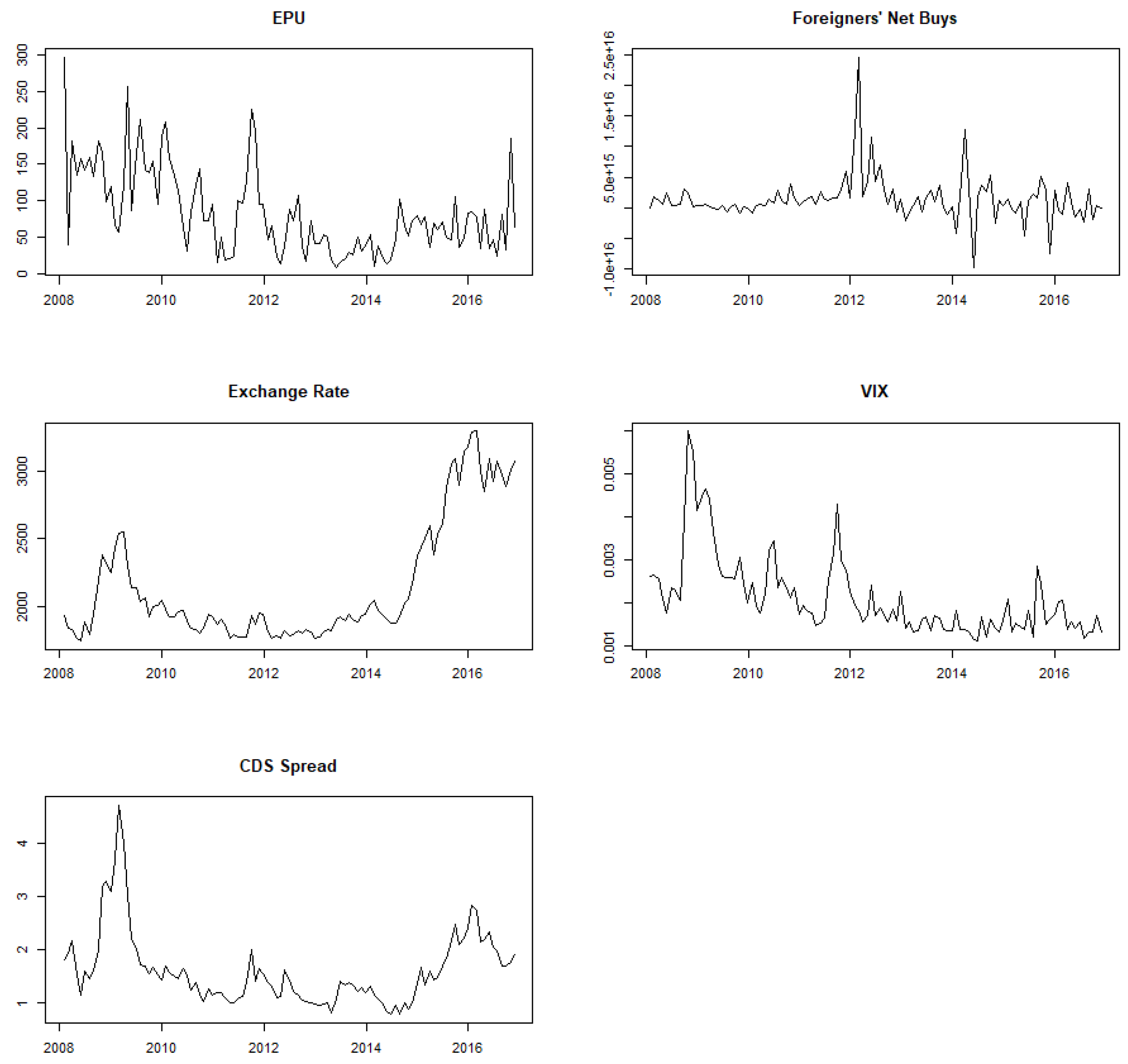
Net buys of foreign investors for each stock are calculated by subtracting the total sales value (in local currency) of the stock, by each investor on a given day, from the total buys, and then aggregating this data on a monthly basis. The dataset includes 8,609,594 ticker-transaction observations (both buys and sells) spanning from January 2, 2008, to November 30, 2016 2. Additionally, I calculate the 21-day rolling return volatility for each stock.
2.2. Methodology
2.2.1. The SVAR model
A VAR model captures the dynamic interactions between economic uncertainty, risk, and investment decision-making without imposing prior restrictions on the structural relationships [16,17,18]. The structural VAR is as follows:
where is a vector containing the following six variables: the percentage change in the EPU index for an opaque market, the change in the VIX index, the change in the CDS spread, the change in the exchange rate, the logarithm of foreigners’ net buys, and the 21-day rolling return volatility. are matrices of coefficients to be estimated, and is a vector of serially and mutually uncorrelated structural innovations. The reduced form of the VAR model is:
where is the vector of estimated residuals in the reduced form. I employ Cholesky ordering, where the EPU index is considered the most exogenous variable and is thus placed first. This first variable affects other variables contemporaneously while being influenced by them with some lag. The second variable is global market risk sentiment, which impacts sovereign risk, the third variable in the ordering. The difference in the exchange rate and foreigners’ net buys are the fourth and fifth variables, respectively. Finally, stock volatility is ordered as the sixth variable. The errors of the reduced form represent linear combinations of the structural errors and can be decomposed into the following components:
where the zero element in the matrix signifies that there is no expected immediate impact from specific shocks, while the nonzero elements represent the coefficients for the i-th response to shocks j. The identified structural innovations and correspond to six types of shocks: changes in economic policy uncertainty, changes in the VIX, changes in the CDS spread, changes in the US dollar exchange rate, changes in the logarithm of foreigners’ net buys, and changes in stock return volatility. I estimate the orthogonalized impulse response functions (IRFs) to assess the impacts of a one-standard-deviation shock from these six influencing factors, along with the forecast error variance decomposition (FEVD) to evaluate the contributions of each factor.
2.2.2. Sudden Price Increases
Stock markets are susceptible to episodes of rapid price increases [19,20,21]. The following is an extension of the Augmented Dickey-Fuller specification used to test for explosivity [22,23]:
The parameters , , and for are to be estimated. The term represents the unobserved random shock, and defines the start and end points of a subsample, where and are expressed as fractions of T.
[24] propose estimating 3 recursively by expanding the end point of the subsamples forward, i.e., by fixing and progressively increasing from a minimum value toward 1. The Augmented Dickey-Fuller statistics are calculated for several values of , and the supremum of these values constitutes the SADF test. The Generalized SADF (GSADF) test allows for flexible window sizes, applying the SADF test to every subperiod by varying both and .
Comparing the statistic with the critical value from the right tail of the limiting distribution provides insight into the null hypothesis versus the alternative . Following [25] and [22], the minimum window size is set to to estimate equation 4 for all possible subsamples, allowing both and to vary. Once exuberant episodes are identified, the supremum of a sequence of backward SADF statistics is computed for each final observation in every regression, yielding the statistic used to estimate the initiation and termination dates of explosive episodes, referred to as the BSADF. Critical values for each test are obtained via Monte Carlo simulations with at least 1,000 replications.
2.3. Probability Model
After identifying episodes of rapid price increases (date-stamping), I perform logistic regression to determine whether economic uncertainty, risk, and foreign investment influenced the likelihood of explosivity in stock prices. Following the approach of [9,26] and [27], I analyze the periods of rapid price increments, represented by a dummy variable , using the following logistic regression:
where the dependent variable is a dummy variable that takes the value of one if , indicating price explosiveness as evidenced by the increase of the BSADF sequence above the corresponding critical value, and zero otherwise. is a vector of parameters to be estimated, and represents a set of explanatory variables.
3. Results
This section presents the main results from the VAR model analysis outlined in Section 2.2.1. The IRFs capture the short-run dynamic responses of the dependent variables to structural shocks. Figure 2 displays the orthogonalized responses of aggregate foreigners’ net buys to positive innovations in the percent changes of the EPU index, using a 5-SVAR system. The significant impact on foreign activity is negative.
This result is further supported by the IRFs from a 6-variable dynamic system, which includes stock return volatility and foreigners’ net buys of individual stocks, as shown in Figure A1 of the Appendix. The analysis uses 90% confidence intervals (CIs), which are considered rigorous. For comparison, [4] use 90% CIs, [28] use 84%, [18] use 68%, and [29] do not rely on CIs. Stability conditions are verified in the Appendix; Figure A16 shows that the estimated VAR model is stable, as all roots lie inside the unit circle.
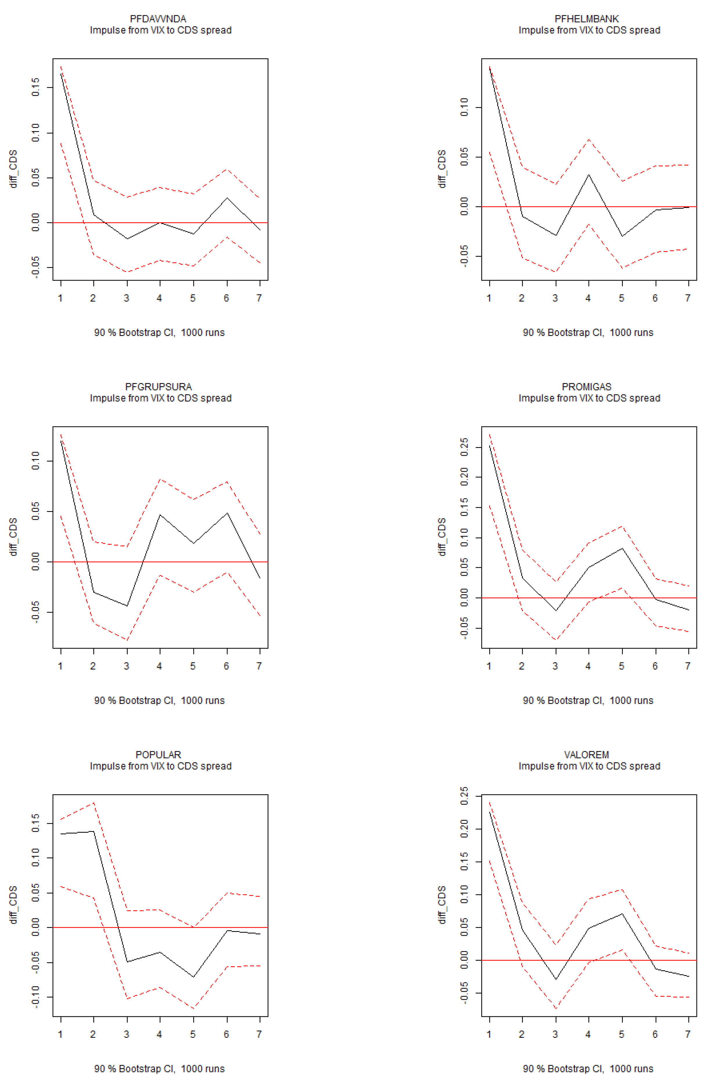
Figure 3 presents the forecast error variance decomposition. Uncertainty plays the most significant role in explaining international activity, surpassing global market volatility as measured by the VIX index. Global market volatility, however, accounts for a substantial portion of the variance in CDS spreads. This result is consistent with the IRFs from the 6-variable dynamic system estimated on individual stocks (Figure A11), where a positive shock to global market volatility significantly increases the CDS spread. Figure 3 and Figure A5 indicate that the CDS spread is relevant for exchange rate movements, with shocks to the CDS spread leading to short-term currency depreciation. Additionally, shocks to the exchange rate are closely linked to individual stocks, as they significantly increase stock return volatility (Figure A7).
The analysis reveals that positive shifts in the Economic Policy Uncertainty (EPU) index significantly reduce foreign investors’ net buying activity, highlighting the stronger influence of localized uncertainty compared to global market volatility. Furthermore, exchange rate shocks substantially affect individual stock volatility, illustrating the sensitivity of domestic markets to external economic factors. Global volatility influences credit default swap (CDS) spreads and exchange rate movements, revealing the interconnected nature of financial risks. However, uncertainty demonstrates a more pronounced impact on international investment activity, emphasizing its central role in speculative and less transparent markets.
Figure 5.
BSADF Tests (Continuation...). Note: Date-stamping of stock price explosiveness.
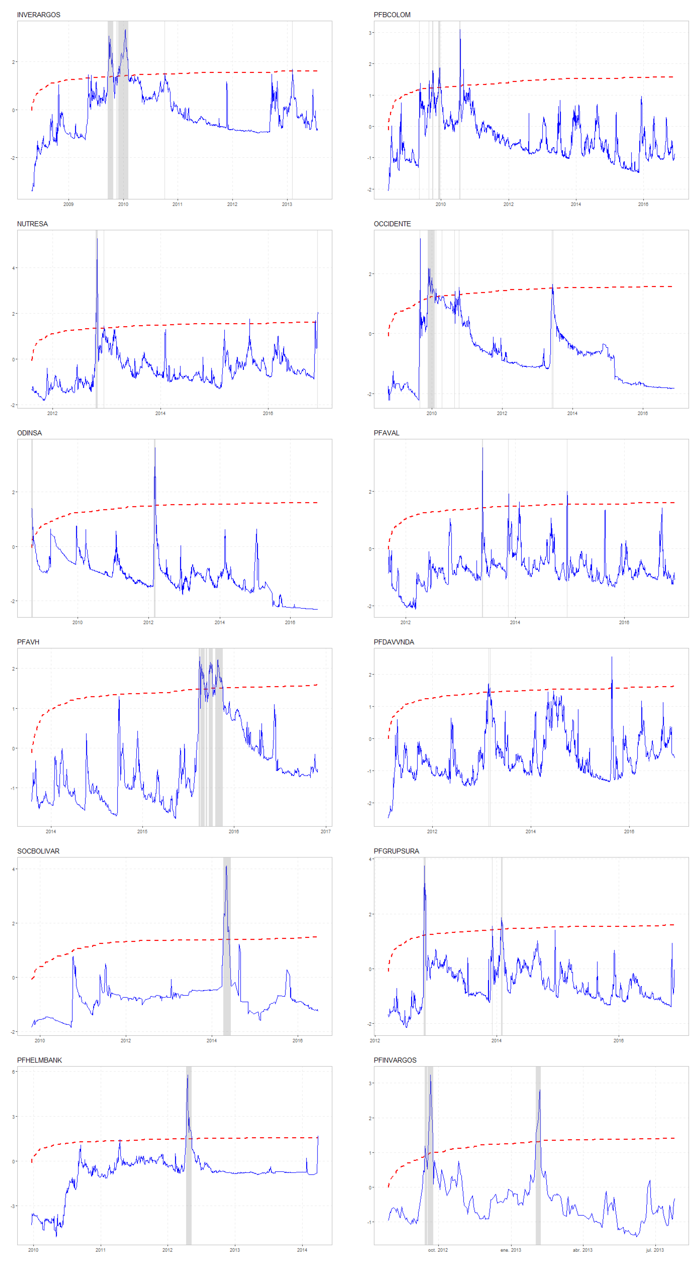
Below, I present the main results from the analysis of price explosiveness outlined in Section 2.3 and Section 2.2.2. Episodes of sudden price increases are identified and displayed in Figure 6, while the results of the probability regression models are shown in Table 1. The dependent variable in these models is a dummy variable , which takes the value of one if . Given that price explosiveness is also related to monetary policy [30,31], the dummy variables and take the value of one during periods of consistent decreases in U.S. and local monetary policy rates, respectively.
Global risk and uncertainty both influence the probability of episodes of accelerating price growth in stocks, as indicated by the statistically positive parameters for the VIX index and the EPU index. Additionally, international investors and monetary policy contribute to explaining episodes of price explosiveness. In contrast, local risk—measured by stock return volatility and the CDS spread—does not appear to drive these rapid price increases. Overall, uncertainty and global risk are the primary factors affecting opaque stock prices.
4. Discussion
Ambiguity in estimating an asset’s value, arising from hard-to-observe risks, is known as uncertainty [7,32,33]. Unlike risk, uncertainty cannot be predicted as there is no clarity on the true probabilistic model [1], while risk refers to uncertainty with a known probability distribution [34]. Uncertainty shocks caused by economic activity and policy reveal the link between different types of financial risks and financial markets [11,35,36,37,38,39]. Incorporating uncertainty is important for asset allocation, as it is significantly correlated with illiquidity [32] and future stock returns at the aggregate level [7,40]. Uncertainty in financial markets, along with the growing linkages and feedback effects between risks and the financial environment, is increasing. This connection has played a key role in driving various recent financial outcomes, including those related to lottery stocks [41] and investor underreaction [42]. At the aggregate level, uncertainty and risk are related. [43] find that uncertainty is related to the Dow Jones volatility and [29] show that while the VIX index does not respond to a Twitter-based market uncertainty index (TMU), a positive shock to the VIX decreases TMU. Researchers puzzled by the mixed empirical findings regarding the relationship between firm opacity and information production in stock markets [44,45] can gain new insights from the analysis of the relation between risk and uncertainty.
Evidence showing that stock markets are susceptible to episodes of rapid price increases is extensive [19,20,21]. Risk and uncertainty are related to explosive episodes in prices, although the literature is not conclusive. In cryptocurrencies, [9] shows that uncertainty exhibits a positive relationship with the probability of price explosiveness, and [46] finds that opacity contributes to speculative bubbles in stock prices. [8] document that the likelihood of sudden price increases in oil prices decreases with heightened uncertainty. Also, [47] argue that the risk premium is related to uncertainty.
Heightened information uncertainty contributes to the price of risk [5] and undermines the stability of financial markets [48]. Emerging stock markets are more opaque than mature stock markets [2], so that during periods of heightened uncertainty, international investors may engage in aggressive trading [4] in emerging economies. Additionally, poor corporate governance and weak prosecution for insider trading contribute to informational inefficiencies [3], and investments in ambiguous assets come with an extra alpha relative to a risky benchmark .
5. Conclusions
Uncertainty and global risk play pivotal roles in shaping financial markets, particularly in emerging economies characterized by informational opacity and structural inefficiencies. This study examines the dynamic relationships between international investors’ activity and measures of uncertainty and risk in an emerging market context, focusing on their influence on net foreign buys, credit default swap (CDS) spreads, exchange rates, and stock return volatility. Using a proprietary dataset of over 8.6 million ticker-transaction observations, this research employs structural vector autoregression (VAR) models and variance decomposition to identify the key drivers of market fluctuations.
The findings reveal that positive innovations in uncertainty, as measured by the Economic Policy Uncertainty (EPU) index, significantly reduce foreign investors’ net buys, a pattern more pronounced than the effects of global market volatility captured by the VIX index. While global volatility is a primary driver of CDS spreads, these spreads are shown to strongly influence exchange rates, leading to short-term currency depreciation. Additionally, heightened uncertainty and global risk contribute to episodes of accelerating price growth, demonstrating their interconnected role in market instability. This paper advances the literature on financial uncertainty by emphasizing its dominant influence over global factors in driving international investment behavior and by highlighting its role in episodes of price explosiveness. The results provide actionable insights for policymakers and investors, underscoring the importance of managing localized uncertainty and global risks in opaque markets.
These findings offer valuable insights for investors and policymakers. They reveal how risk and uncertainty drive rapid price growth, particularly in opaque markets where external conditions dominate. Addressing these challenges requires stronger regulatory frameworks, improved transparency, and measures to mitigate the disruptive effects of uncertainty on financial systems.
Funding
This research received no external funding
Data Availability Statement
The data supporting the findings of this study are publicly available from the Economic Policy Uncertainty website (https://www.policyuncertainty.com/). Measures of risk are available through Bloomberg Terminals; however, access to these data is restricted, as they were used under license for this study and are not publicly available. Data on public companies, such as ticker-transaction observations (both buys and sells) and type of investor, were kindly provided by Diego Agudelo at Universidad EAFIT. Due to restrictions on these data, public financial information must be sourced through alternative providers.
Acknowledgments
I thank Diego Agudelo at the Area of Macroeconomics and Finance at Universidad EAFIT for providing proprietary data on the stock market. I am also very grateful for his insightful comments.
Conflicts of Interest
The author declare no conflicts of interest.
Abbreviations
The following abbreviations are used in this manuscript:
| CDS | Credit Default Swap |
| VIX | CBOE Volatility Index |
| EPU | Economic Policy Uncertainty Index |
| 6-SVAR | 6-variable structural vector autorregression |
| GSADF | Generalized Supremum Augmented Dickey-Fuller test |
Appendix A
Figure A1.
IRFs of Uncertainty to Foreigners’ Activity. Note: Impulse response functions (IRFs) for the structural VAR system of six variables over a six-month horizon. The 90% confidence intervals are displayed in red.
Figure A1.
IRFs of Uncertainty to Foreigners’ Activity. Note: Impulse response functions (IRFs) for the structural VAR system of six variables over a six-month horizon. The 90% confidence intervals are displayed in red.
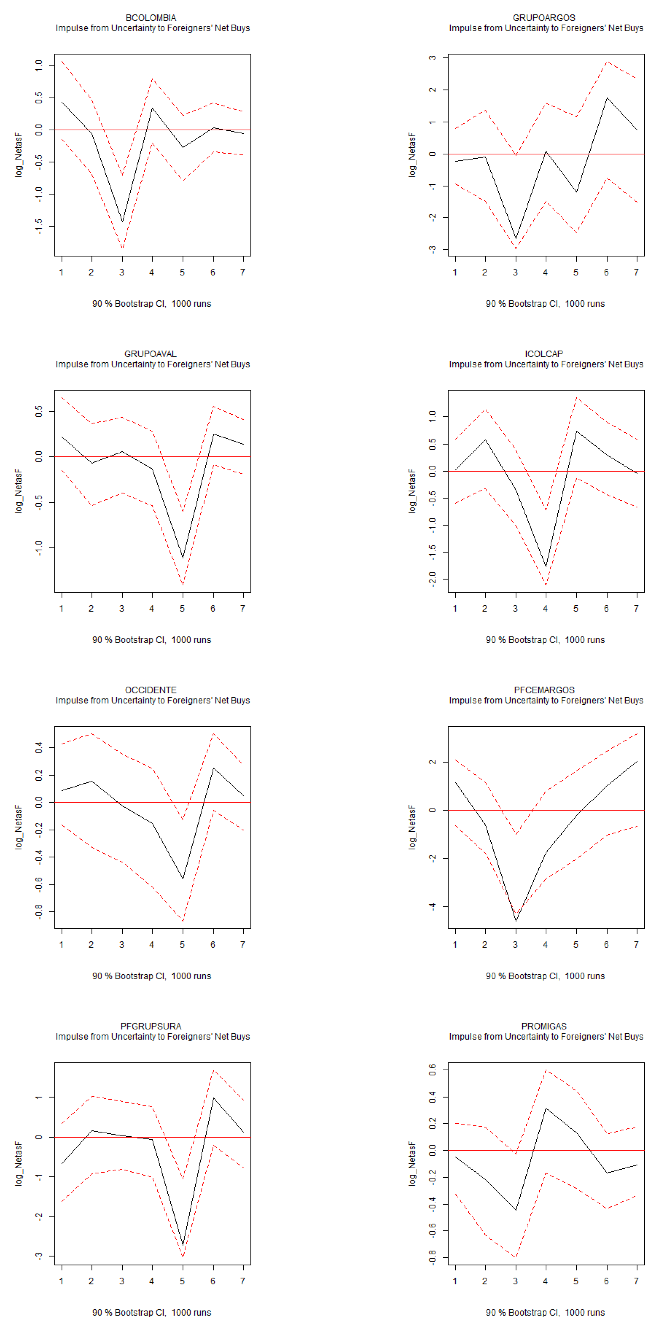
Figure A2.
IRFs of CDS Spreads to Exchange Rate. Note: Impulse response functions (IRFs) for the structural VAR system of six variables over a six-month horizon. The 90% confidence intervals are displayed in red.
Figure A2.
IRFs of CDS Spreads to Exchange Rate. Note: Impulse response functions (IRFs) for the structural VAR system of six variables over a six-month horizon. The 90% confidence intervals are displayed in red.
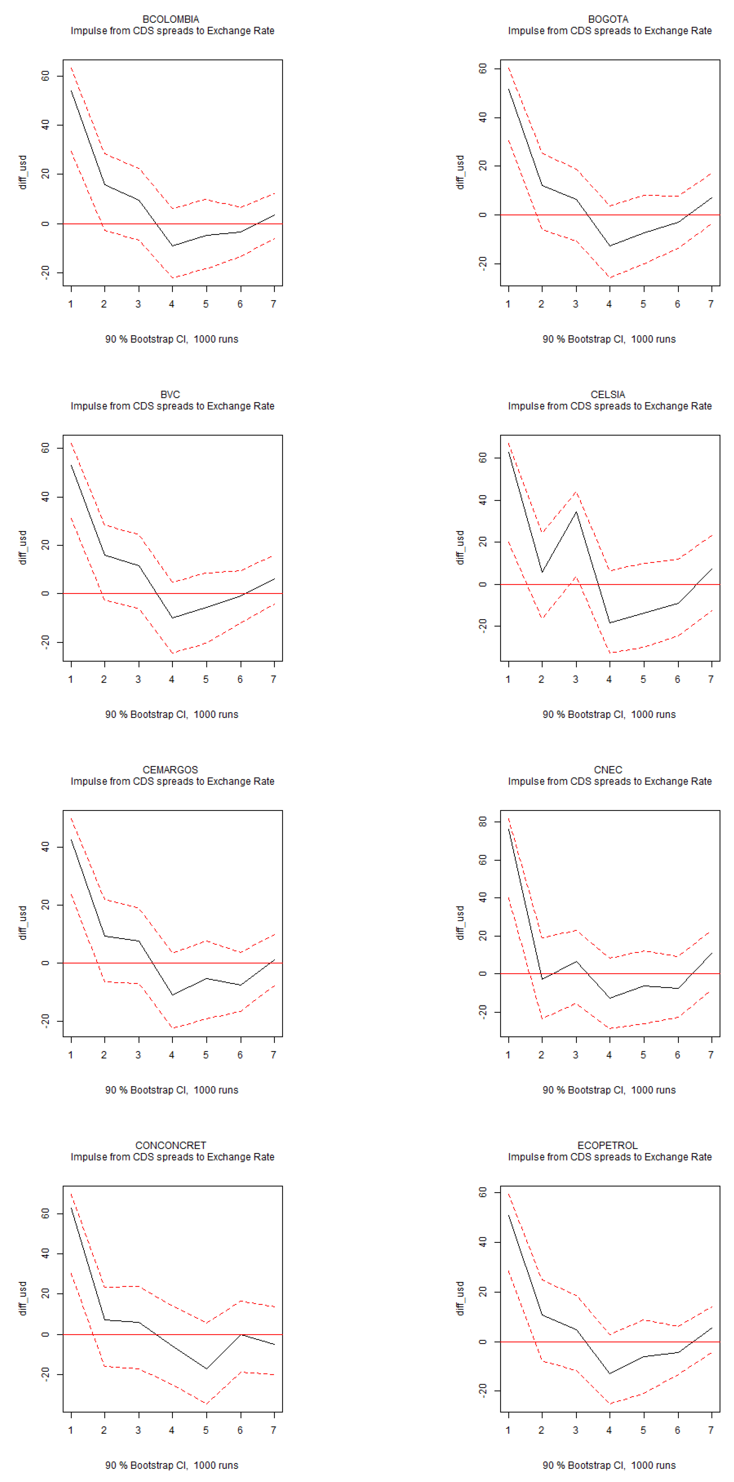
Figure A3.
IRFs of CDS Spreads to Exchange Rate (Continuation...). Note: Impulse response functions (IRFs) for the structural VAR system of six variables over a six-month horizon. The 90% confidence intervals are displayed in red.
Figure A3.
IRFs of CDS Spreads to Exchange Rate (Continuation...). Note: Impulse response functions (IRFs) for the structural VAR system of six variables over a six-month horizon. The 90% confidence intervals are displayed in red.
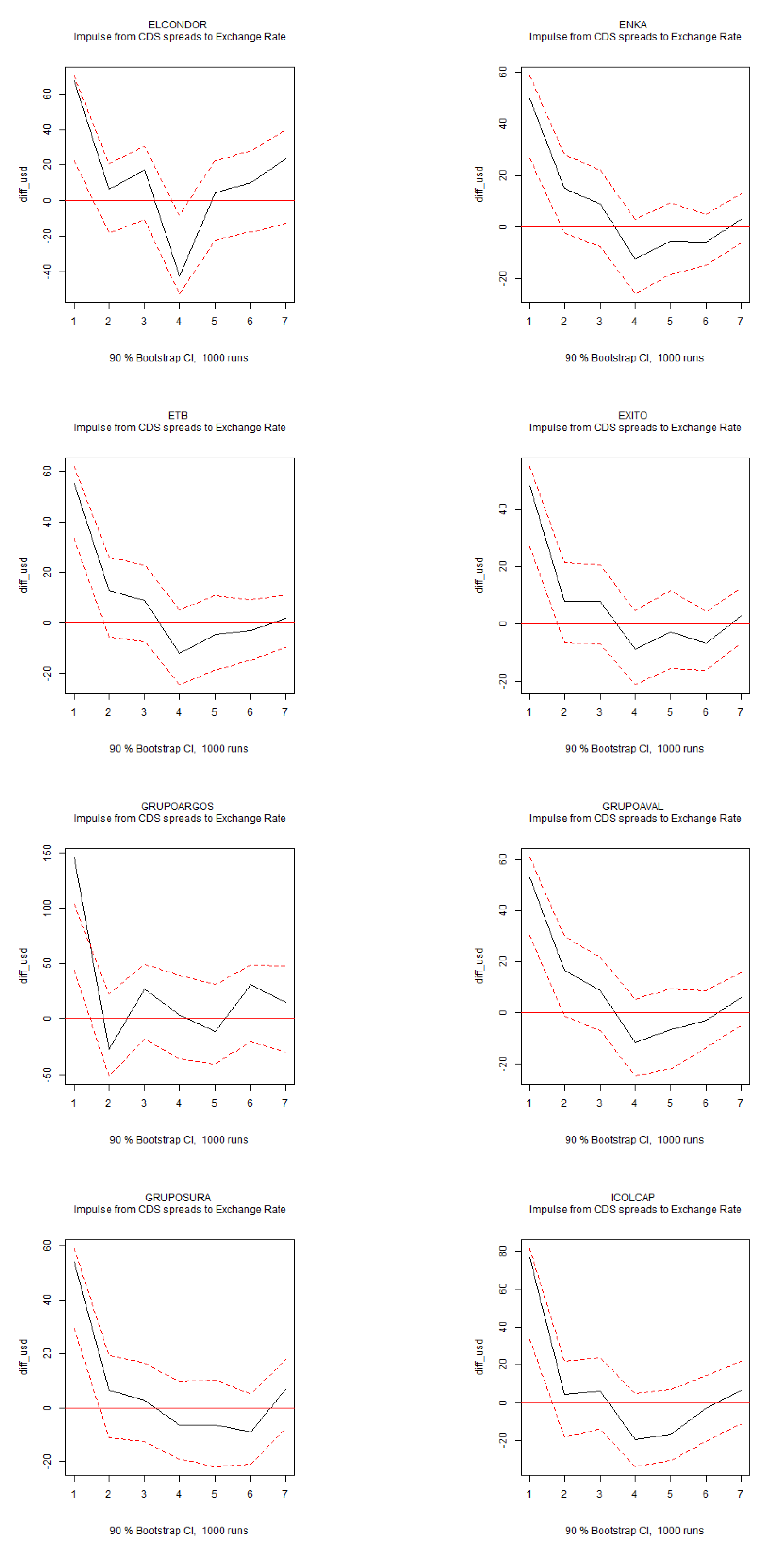
Figure A4.
IRFs of CDS Spreads to Exchange Rate (Continuation...). Note: Impulse response functions (IRFs) for the structural VAR system of six variables over a six-month horizon. The 90% confidence intervals are displayed in red.
Figure A4.
IRFs of CDS Spreads to Exchange Rate (Continuation...). Note: Impulse response functions (IRFs) for the structural VAR system of six variables over a six-month horizon. The 90% confidence intervals are displayed in red.
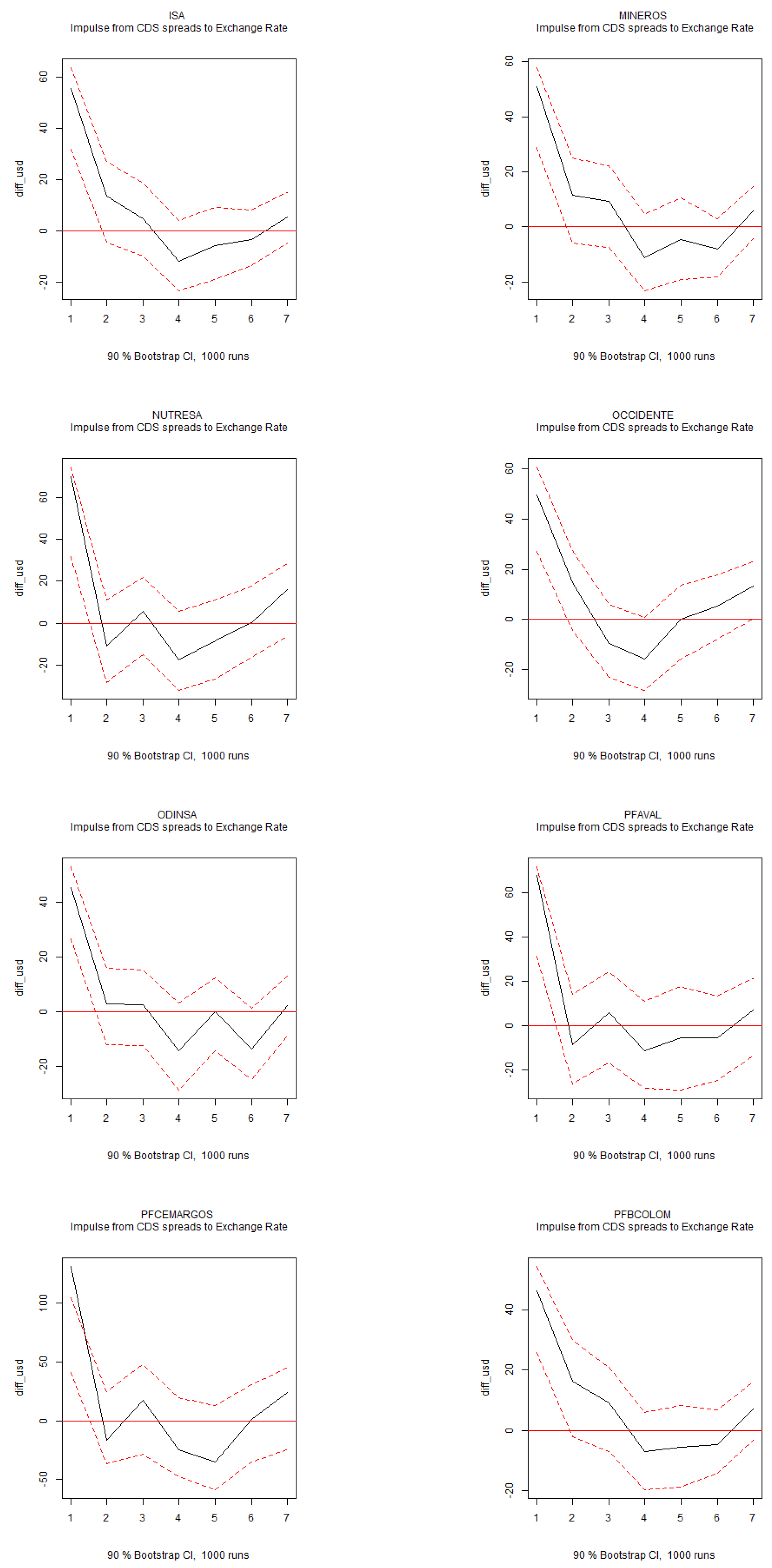
Figure A5.
IRFs of CDS Spreads to Exchange Rate (Continuation...). Note: Impulse response functions (IRFs) for the structural VAR system of six variables over a six-month horizon. The 90% confidence intervals are displayed in red.
Figure A5.
IRFs of CDS Spreads to Exchange Rate (Continuation...). Note: Impulse response functions (IRFs) for the structural VAR system of six variables over a six-month horizon. The 90% confidence intervals are displayed in red.
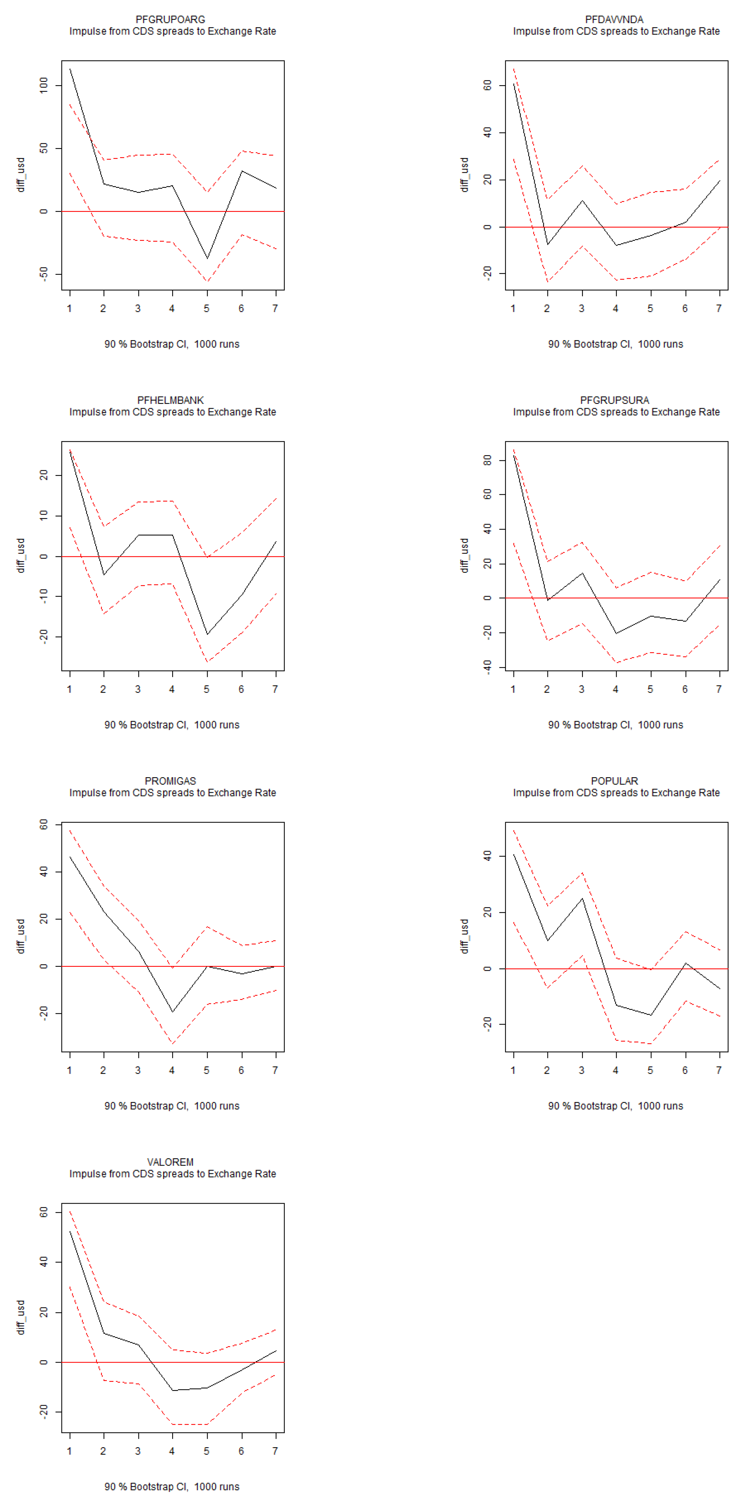
Figure A6.
IRFs of Exchange Rate to Stock Return Volatility. Note: Impulse response functions (IRFs) for the structural VAR system of six variables over a six-month horizon. The 90% confidence intervals are displayed in red.
Figure A6.
IRFs of Exchange Rate to Stock Return Volatility. Note: Impulse response functions (IRFs) for the structural VAR system of six variables over a six-month horizon. The 90% confidence intervals are displayed in red.
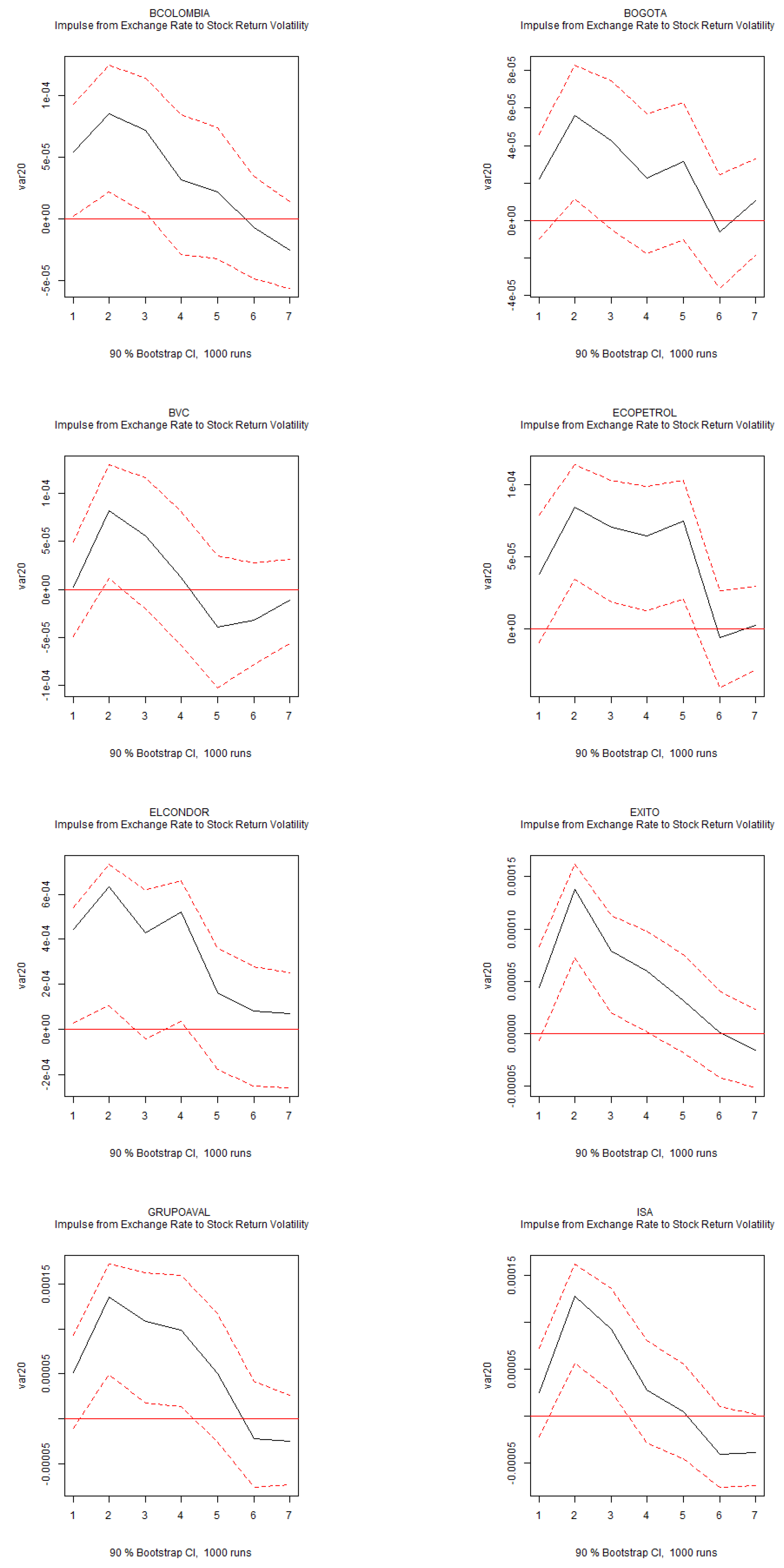
Figure A7.
IRFs of Exchange Rate to Stock Return Volatility (Continuation...). Note: Impulse response functions (IRFs) for the structural VAR system of six variables over a six-month horizon. The 90% confidence intervals are displayed in red.
Figure A7.
IRFs of Exchange Rate to Stock Return Volatility (Continuation...). Note: Impulse response functions (IRFs) for the structural VAR system of six variables over a six-month horizon. The 90% confidence intervals are displayed in red.
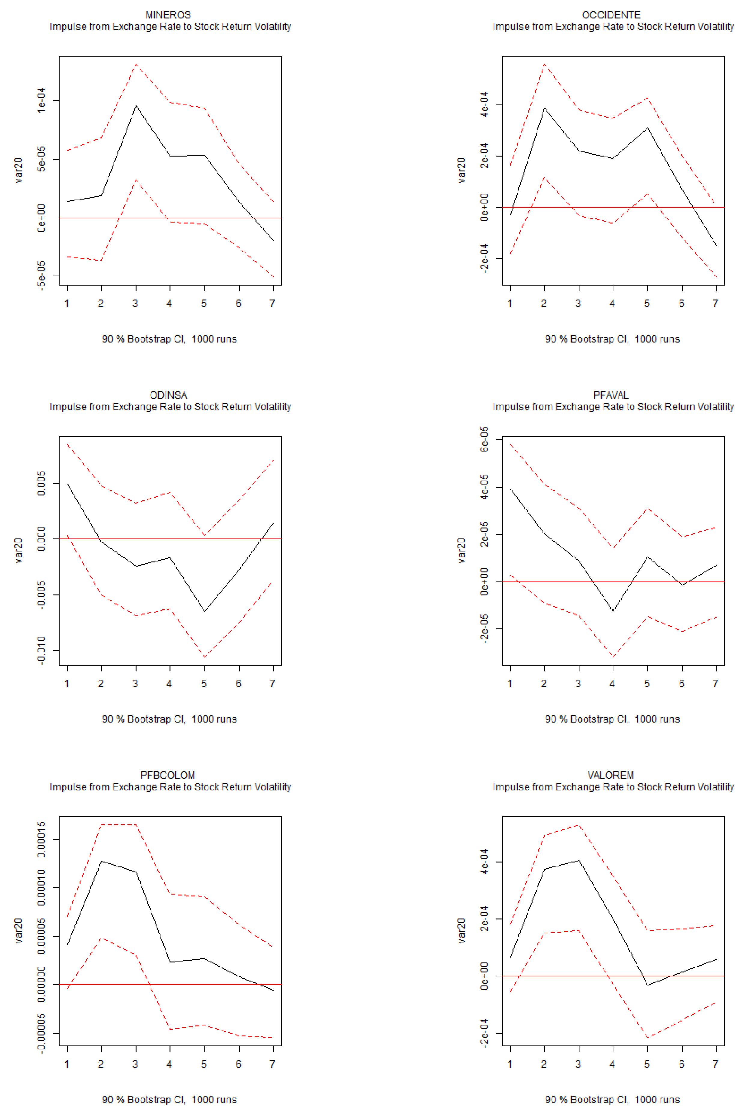
Figure A8.
IRFs of VIX to CDS Spread. Note: Impulse response functions (IRFs) for the structural VAR system of six variables over a six-month horizon. The 90% confidence intervals are displayed in red.
Figure A8.
IRFs of VIX to CDS Spread. Note: Impulse response functions (IRFs) for the structural VAR system of six variables over a six-month horizon. The 90% confidence intervals are displayed in red.
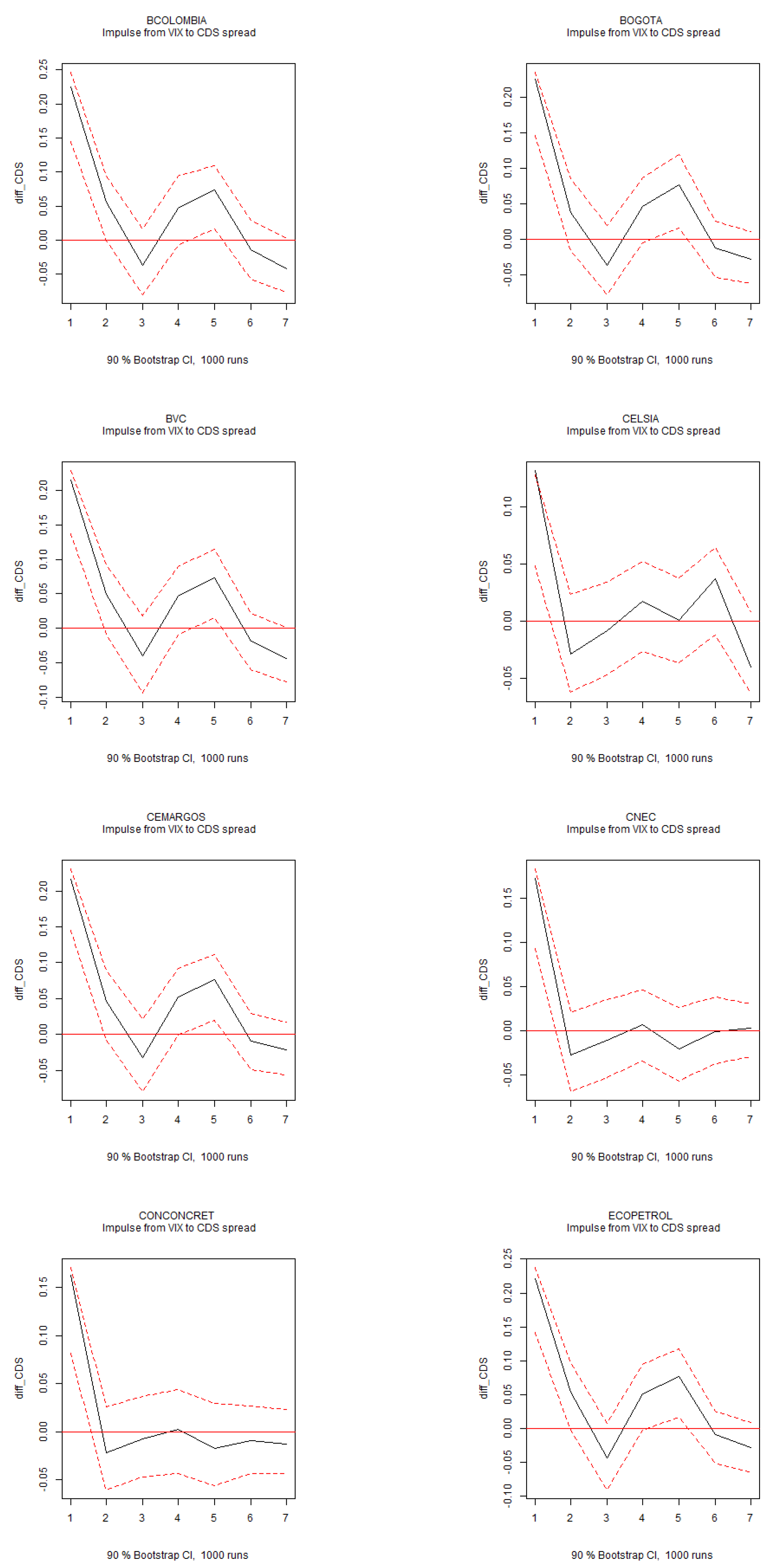
Figure A9.
IRFs of VIX to CDS Spread (Continuation...). Note: Impulse response functions (IRFs) for the structural VAR system of six variables over a six-month horizon. The 90% confidence intervals are displayed in red.
Figure A9.
IRFs of VIX to CDS Spread (Continuation...). Note: Impulse response functions (IRFs) for the structural VAR system of six variables over a six-month horizon. The 90% confidence intervals are displayed in red.
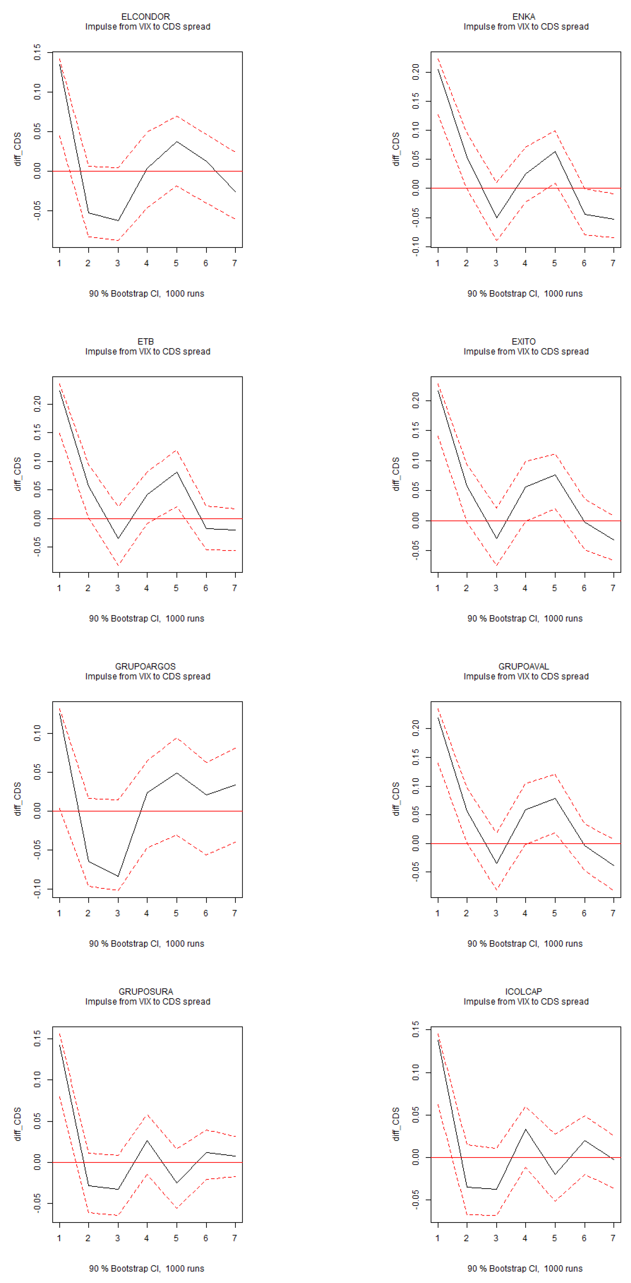
Figure A10.
IRFs of VIX to CDS Spread (Continuation...). Note: Impulse response functions (IRFs) for the structural VAR system of six variables over a six-month horizon. The 90% confidence intervals are displayed in red.
Figure A10.
IRFs of VIX to CDS Spread (Continuation...). Note: Impulse response functions (IRFs) for the structural VAR system of six variables over a six-month horizon. The 90% confidence intervals are displayed in red.
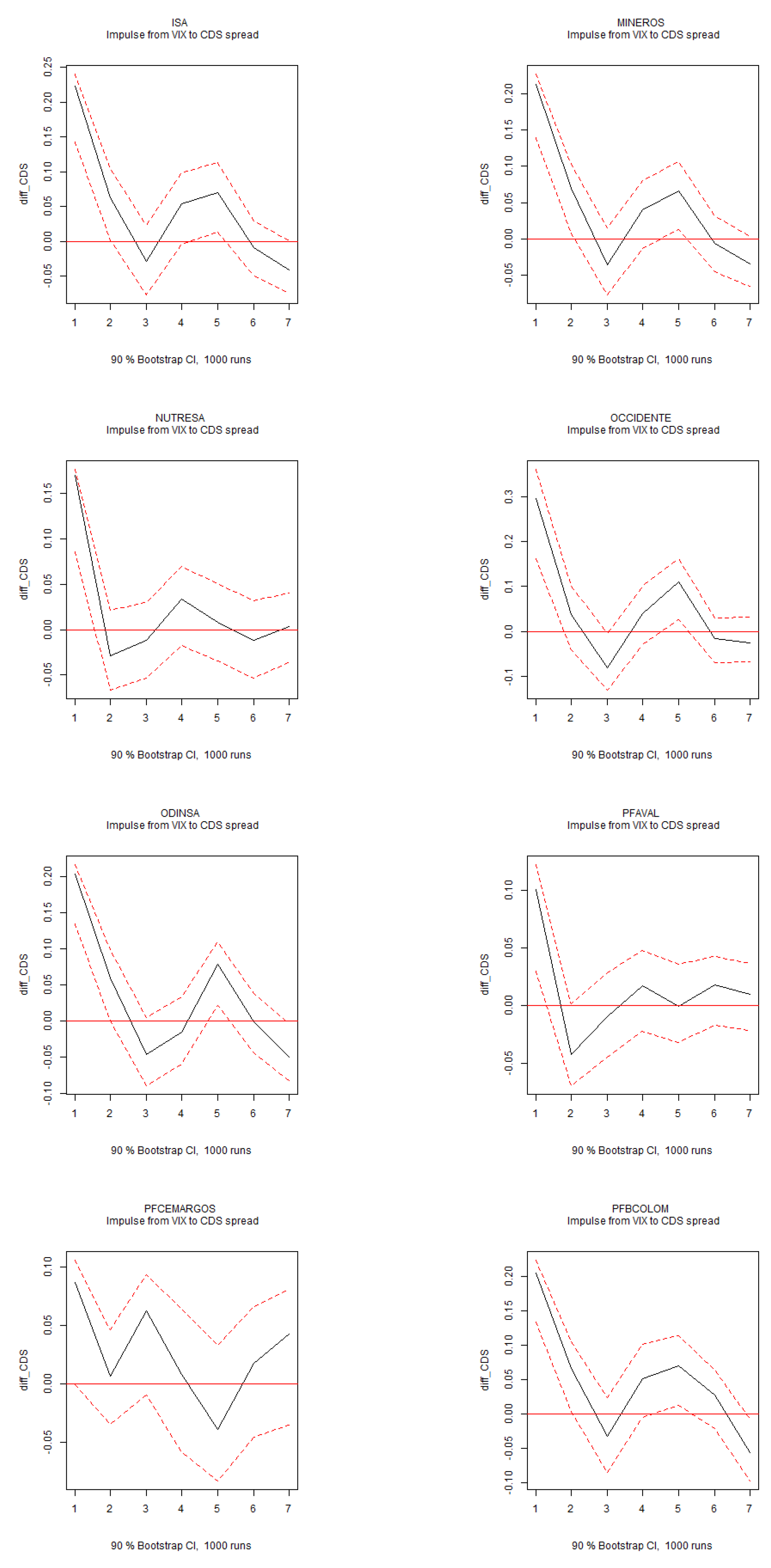
Figure A11.
IRFs of VIX to CDS Spread (Continuation...). Note: Impulse response functions (IRFs) for the structural VAR system of six variables over a six-month horizon. The 90% confidence intervals are displayed in red.
Figure A11.
IRFs of VIX to CDS Spread (Continuation...). Note: Impulse response functions (IRFs) for the structural VAR system of six variables over a six-month horizon. The 90% confidence intervals are displayed in red.
Appendix B
Figure A12.
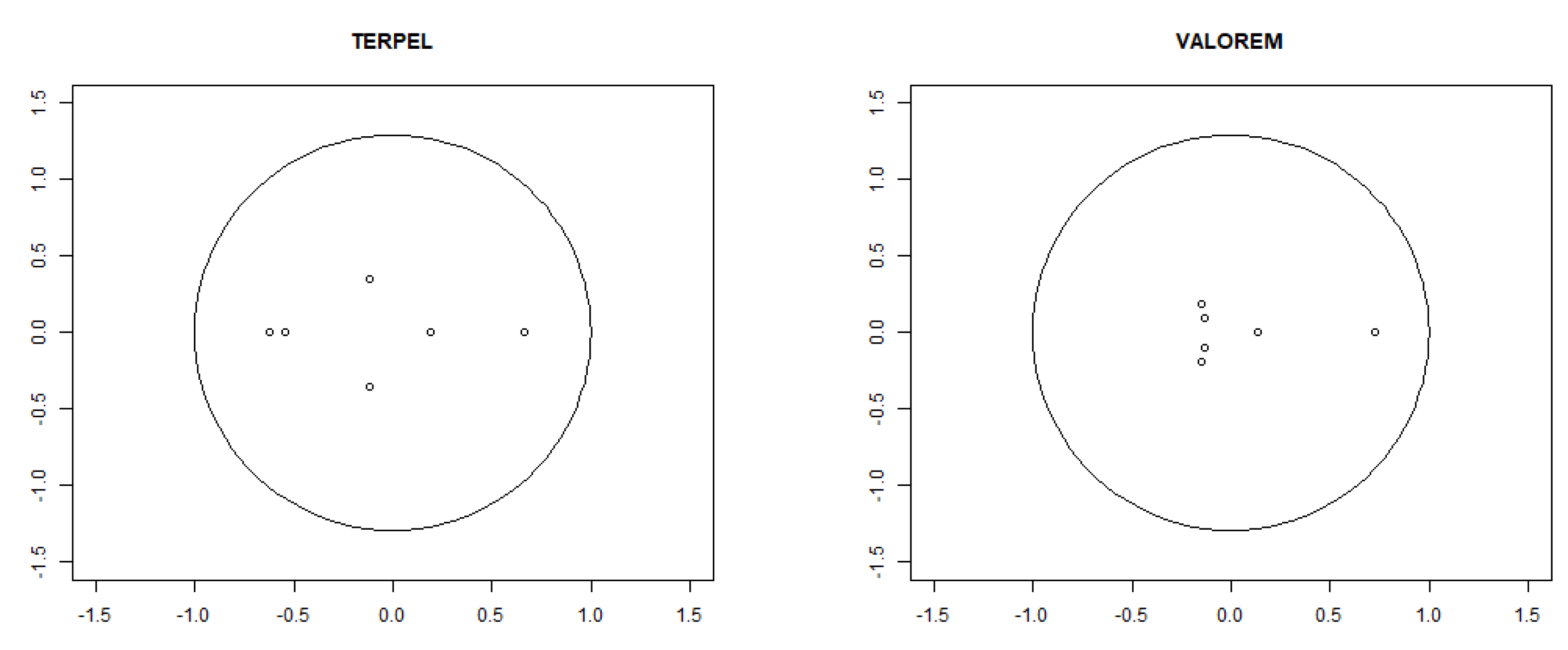
Stationarity. Note: Structural VAR stability condition: All eigenvalues lie within the unit circle, indicating the stability of the SVAR model.
Figure A12.
Stationarity. Note: Structural VAR stability condition: All eigenvalues lie within the unit circle, indicating the stability of the SVAR model.
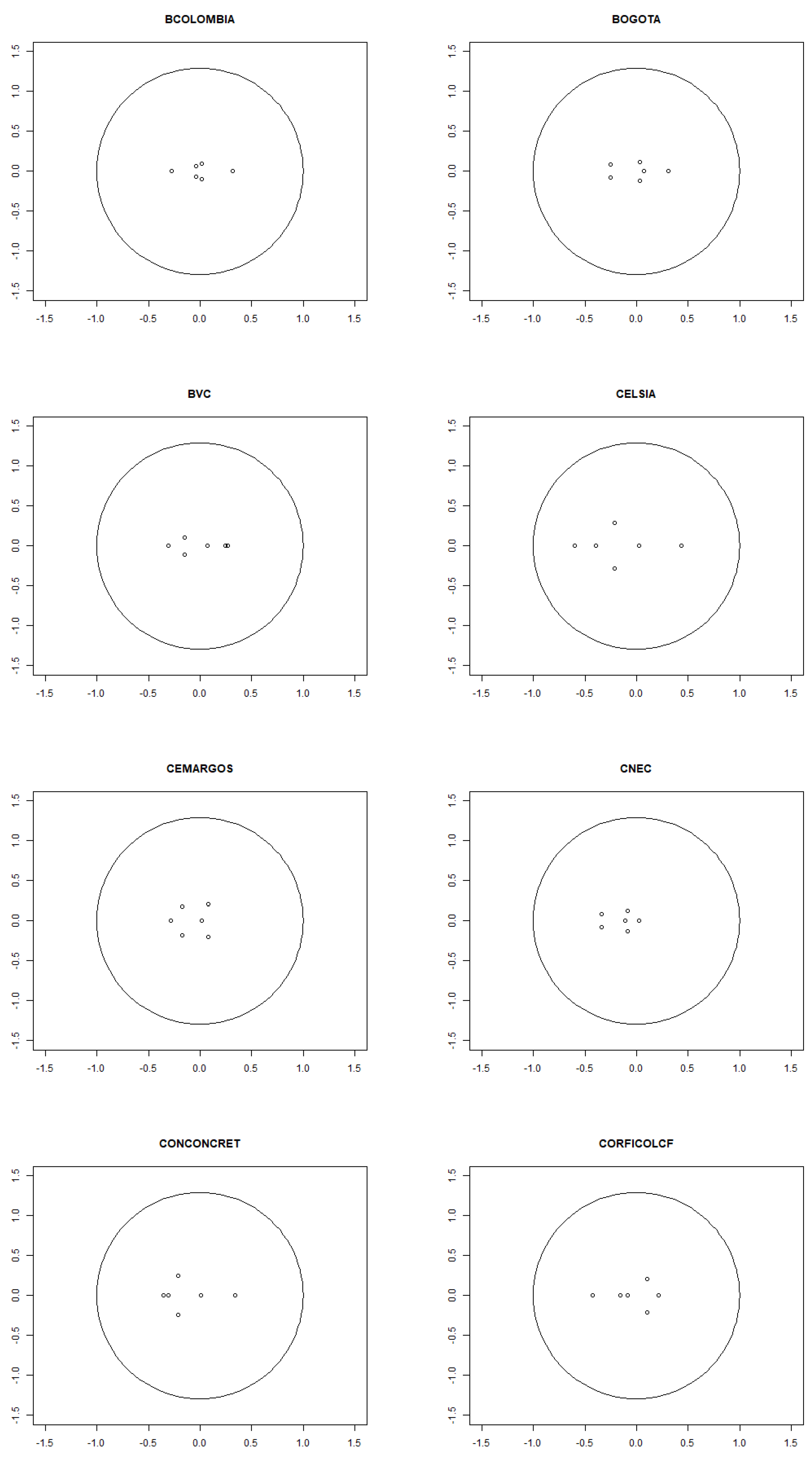
Figure A13.
Stationarity (Continuation...). Note: Structural VAR stability condition: All eigenvalues lie within the unit circle, indicating the stability of the SVAR model.
Figure A13.
Stationarity (Continuation...). Note: Structural VAR stability condition: All eigenvalues lie within the unit circle, indicating the stability of the SVAR model.
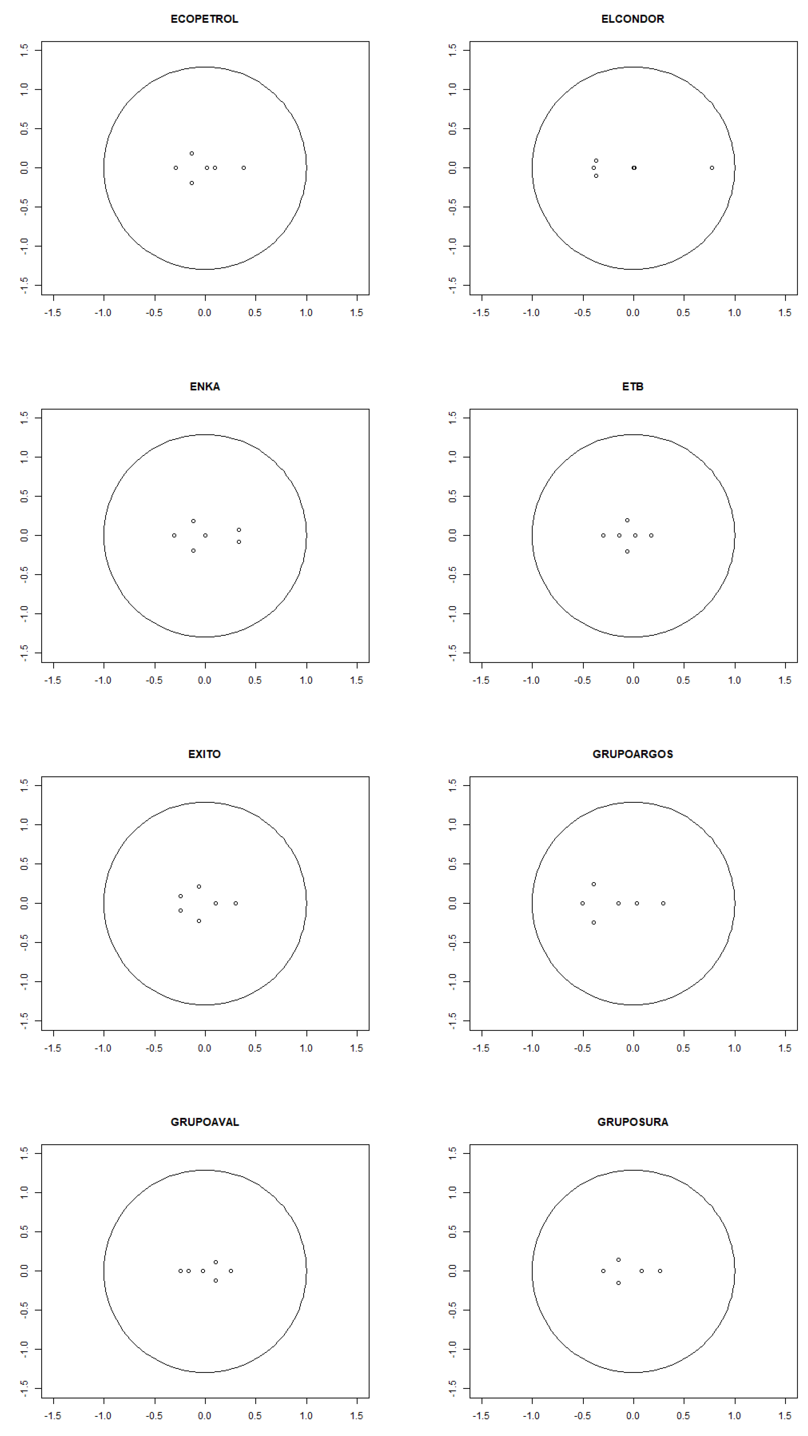
Figure A14.
Stationarity (Continuation...). Note: Structural VAR stability condition: All eigenvalues lie within the unit circle, indicating the stability of the SVAR model.
Figure A14.
Stationarity (Continuation...). Note: Structural VAR stability condition: All eigenvalues lie within the unit circle, indicating the stability of the SVAR model.
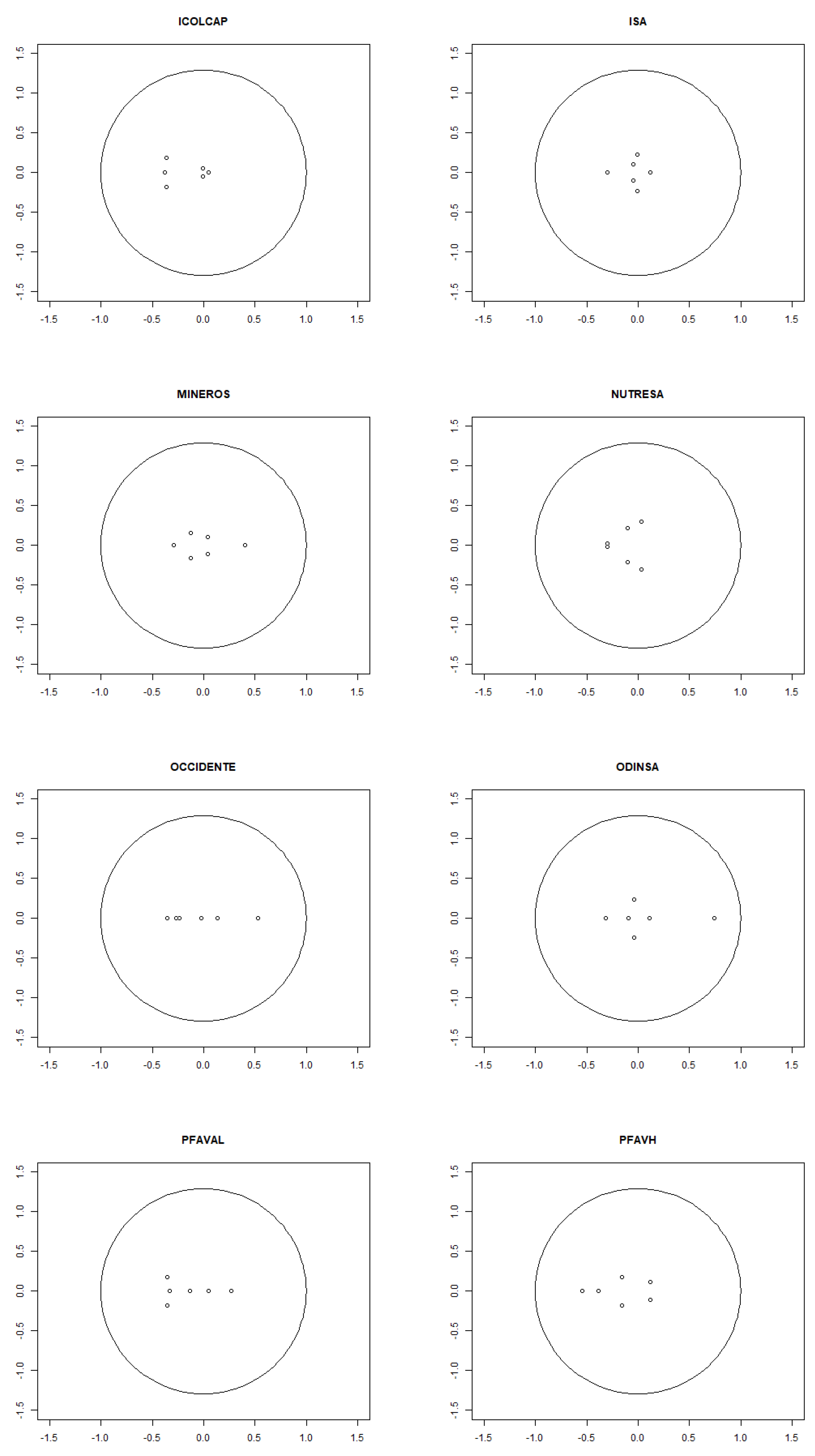
Figure A15.
Stationarity (Continuation...). Note: Structural VAR stability condition: All eigenvalues lie within the unit circle, indicating the stability of the SVAR model.
Figure A15.
Stationarity (Continuation...). Note: Structural VAR stability condition: All eigenvalues lie within the unit circle, indicating the stability of the SVAR model.
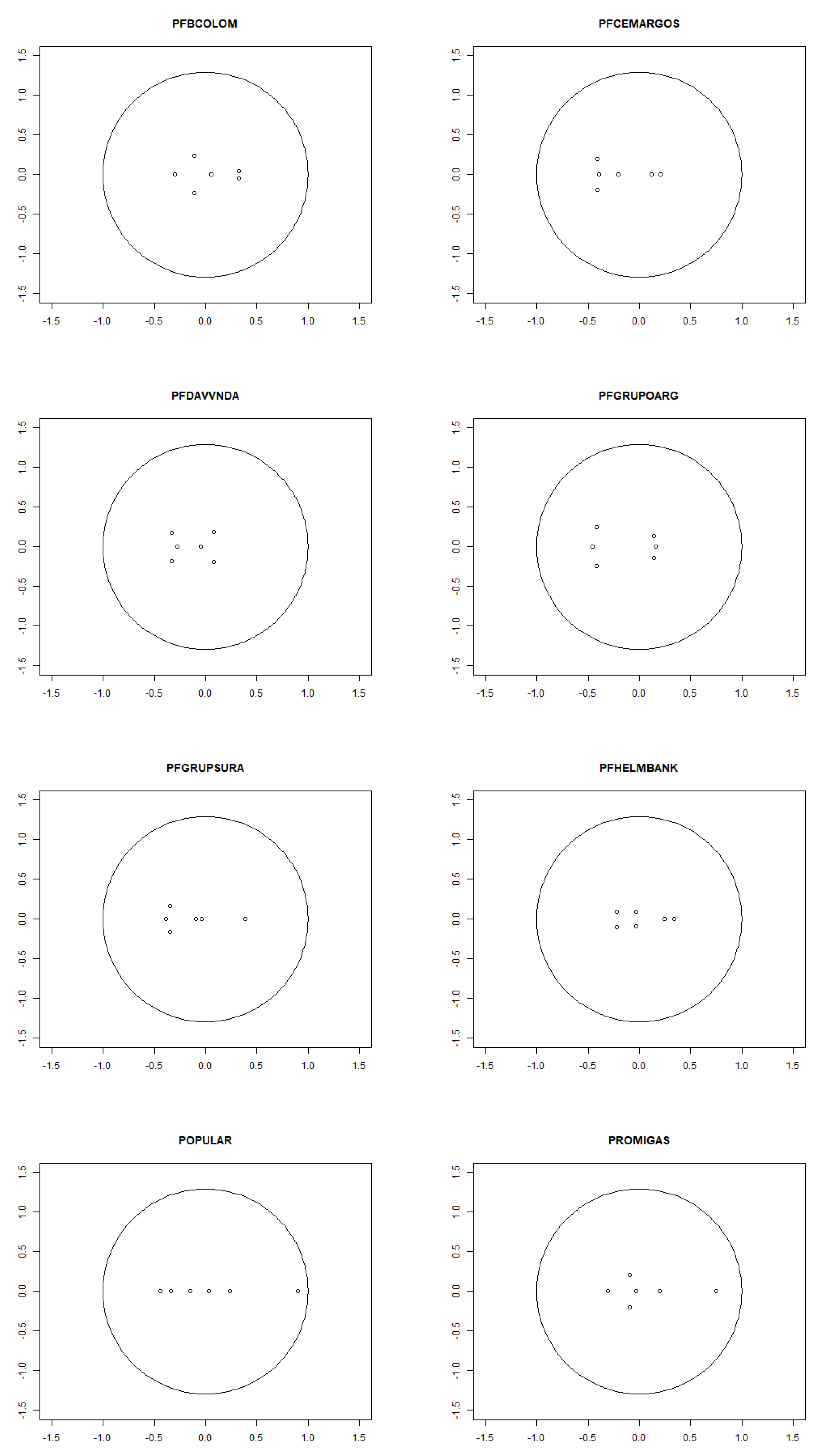
Figure A16.
Stationarity (Continuation...). Note: Structural VAR stability condition: All eigenvalues lie within the unit circle, indicating the stability of the SVAR model.
Figure A16.
Stationarity (Continuation...). Note: Structural VAR stability condition: All eigenvalues lie within the unit circle, indicating the stability of the SVAR model.
References
- Maccheroni, F.; Marinacci, M.; Ruffino, D. Alpha as ambiguity: Robust mean-variance portfolio analysis. Econometrica 2013, 81, 1075–1113. [Google Scholar] [CrossRef]
- Morck, R.; Yeung, B.; Yu, W. The Information Content of Stock Markets: Why do Emerging Markets have Synchronous Stock Price. Journal of Financial Economics 2000, 58, 215–260. [Google Scholar] [CrossRef]
- González, M.; Astaíza-Gómez, J.G.; Pantoja, J. Actively managed equity mutual funds in emerging markets. Research in International Business and Finance 2024, 72, 102540. [Google Scholar] [CrossRef]
- Múnera, D.J.; Agudelo, D.A. Who moved my liquidity? Liquidity evaporation in emerging markets in periods of financial uncertainty. Journal of International Money and Finance 2022, 129, 102723. [Google Scholar] [CrossRef]
- Hansen, L.P.; Sargent, T.J. Fragile beliefs and the price of uncertainty. Quantitative Economics 2010, 1, 129–162. [Google Scholar]
- Morgan, D.P. Rating banks: Risk and uncertainty in an opaque industry. American Economic Review 2002, 92, 874–888. [Google Scholar] [CrossRef]
- Jiang, G.; Lee, C.M.; Zhang, Y. Information uncertainty and expected returns. Review of Accounting Studies 2005, 10, 185–221. [Google Scholar] [CrossRef]
- Mamman, S.O.; Iliyasu, J.; Ahmed, U.A.; Salami, F. Global uncertainties, geopolitical risks and price exuberance: Evidence from international energy market. OPEC Energy Review 2024. [Google Scholar] [CrossRef]
- Enoksen, F.A.; Landsnes, C.J.; Lučivjanská, K.; Molnár, P. Understanding risk of bubbles in cryptocurrencies. Journal of Economic Behavior & Organization 2020, 176, 129–144. [Google Scholar]
- Liang, C.; Umar, M.; Ma, F.; Huynh, T.L. Climate policy uncertainty and world renewable energy index volatility forecasting. Technological Forecasting and Social Change 2022, 182, 121810. [Google Scholar] [CrossRef]
- Silva, F.; Ferreira, A.; Cortez, M.C. The performance of green bond portfolios under climate uncertainty: A comparative analysis with conventional and black bond portfolios. Research in International Business and Finance 2024, 70, 102354. [Google Scholar] [CrossRef]
- Baker, S.R.; Bloom, N.; Davis, S.J. Measuring economic policy uncertainty. The quarterly journal of economics 2016, 131, 1593–1636. [Google Scholar] [CrossRef]
- Perico Ortiz, D. Measuring Economic Policy Uncertainty in Colombia: a News Based Approach. Available at SSRN 4193944 2018. [Google Scholar] [CrossRef]
- Brunnermeier, M.K.; Pedersen, L.H. Market liquidity and funding liquidity. The review of financial studies 2009, 22, 2201–2238. [Google Scholar] [CrossRef]
- Neaime, S.; Gaysset, I. Macroeconomic and monetary policy responses in selected highly indebted MENA countries post Covid 19: A structural VAR approach. Research in International Business and Finance 2022, 61, 101674. [Google Scholar] [CrossRef]
- Sims, C.A. Macroeconomics and reality. Econometrica: journal of the Econometric Society 1980, 1–48. [Google Scholar] [CrossRef]
- Stock, J.H.; Watson, M.W. Vector autoregressions. Journal of Economic perspectives 2001, 15, 101–115. [Google Scholar] [CrossRef]
- Gholipour, H.F.; Tajaddini, R.; Farzanegan, M.R.; Yam, S. Responses of REITs index and commercial property prices to economic uncertainties: A VAR analysis. Research in International Business and Finance 2021, 58, 101457. [Google Scholar] [CrossRef]
- Lehnert, T. Fear and stock price bubbles. Plos one 2020, 15, e0233024. [Google Scholar] [CrossRef] [PubMed]
- Diba, B.T.; Grossman, H.I. Explosive rational bubbles in stock prices? The American Economic Review 1988, 78, 520–530. [Google Scholar]
- Dezhbakhsh, H.; Demirguc-Kunt, A. On the presence of speculative bubbles in stock prices. Journal of Financial and Quantitative Analysis 1990, 25, 101–112. [Google Scholar] [CrossRef]
- Phillips, P.C.; Shi, S.; Yu, J. Testing for multiple bubbles: Limit theory of real-time detectors. International Economic Review 2015, 56, 1079–1134. [Google Scholar] [CrossRef]
- Gomez-Gonzalez, J.E.; Gamboa-Arbeláez, J.; Hirs-Garzón, J.; Pinchao-Rosero, A. When bubble meets bubble: Contagion in OECD countries. The Journal of Real Estate Finance and Economics 2018, 56, 546–566. [Google Scholar] [CrossRef]
- Phillips, P.C.; Wu, Y.; Yu, J. Explosive behavior in the 1990s Nasdaq: When did exuberance escalate asset values? International economic review 2011, 52, 201–226. [Google Scholar] [CrossRef]
- Phillips, P.C.; Shi, S.; Yu, J. Testing for multiple bubbles: Historical episodes of exuberance and collapse in the S&P 500. International economic review 2015, 56, 1043–1078. [Google Scholar]
- Bouri, E.; Shahzad, S.J.H.; Roubaud, D. Co-explosivity in the cryptocurrency market. Finance Research Letters 2019, 29, 178–183. [Google Scholar] [CrossRef]
- Shahzad, S.J.H.; Anas, M.; Bouri, E. Price explosiveness in cryptocurrencies and Elon Musk’s tweets. Finance Research Letters 2022, 47, 102695. [Google Scholar] [CrossRef]
- Gomez-Gonzalez, J.E.; Hirs-Garzón, J.; Uribe, J.M. Interdependent capital structure choices and the macroeconomy. The North American Journal of Economics and Finance 2022, 62, 101750. [Google Scholar] [CrossRef]
- Chatterjee, U.; French, J.J. A note on tweeting and equity markets before and during the Covid-19 pandemic. Finance Research Letters 2022, 46, 102224. [Google Scholar] [CrossRef]
- Okina, K.; Shirakawa, M.; Shiratsuka, S. The asset price bubble and monetary policy: Japan’s experience in the late 1980s and the lessons. Monetary and Economic Studies (special edition) 2001, 19, 395–450. [Google Scholar]
- Jarrow, R.; Lamichhane, S. Risk premia, asset price bubbles, and monetary policy. Journal of Financial Stability 2022, 60, 101005. [Google Scholar] [CrossRef]
- Kang, W.; Li, N.; Zhang, H. Information uncertainty and the pricing of liquidity. Journal of Empirical Finance 2019, 54, 77–96. [Google Scholar] [CrossRef]
- Zhang, X.F. Information uncertainty and stock returns. Journal of Finance 2006, 61, 105–136. [Google Scholar] [CrossRef]
- Watkins, G.P. Knight’s risk, uncertainty and profit. The Quarterly Journal of Economics 1922, 36, 682–690. [Google Scholar] [CrossRef]
- Aggarwal, R.; Goodell, J.W. Cross-national differences in access to finance: Influence of culture and institutional environments. Research in International Business and Finance 2014, 31, 193–211. [Google Scholar] [CrossRef]
- Awijen, H.; Zaied, Y.B.; Lahouel, B.B.; Khlifi, F. Machine learning for US cross-industry return predictability under information uncertainty. Research in International Business and Finance 2023, 64, 101893. [Google Scholar] [CrossRef]
- Cesa-Bianchi, A.; Pesaran, M.H.; Rebucci, A. Uncertainty and economic activity: A multicountry perspective. The Review of Financial Studies 2020, 33, 3393–3445. [Google Scholar] [CrossRef]
- Chen, Z.; Petkova, R. Does idiosyncratic volatility proxy for risk exposure? The Review of Financial Studies 2012, 25, 2745–2787. [Google Scholar] [CrossRef]
- Gennaioli, N.; Shleifer, A.; Vishny, R. „Market institution, financial market risk and financial crisis. Journal of financial economics 2012, 104, 452–468. [Google Scholar] [CrossRef]
- Hao, X.; Wang, Y.; Wu, C.; Wu, L. Oil information uncertainty and aggregate market returns: A natural experiment based on satellite data. Journal of Financial Markets 2024, 100913. [Google Scholar] [CrossRef]
- Tao, R.; Brooks, C.; Bell, A.R. When is a MAX not the MAX? How news resolves information uncertainty. Journal of Empirical Finance 2020, 57, 33–51. [Google Scholar] [CrossRef]
- Jia, N.; Rai, A.; Xu, S.X. Reducing capital market anomaly: The role of information technology using an information uncertainty lens. Management Science 2020, 66, 979–1001. [Google Scholar] [CrossRef]
- Sharif, A.; Aloui, C.; Yarovaya, L. COVID-19 pandemic, oil prices, stock market, geopolitical risk and policy uncertainty nexus in the US economy: Fresh evidence from the wavelet-based approach. International review of financial analysis 2020, 70, 101496. [Google Scholar] [CrossRef]
- Derrien, F.; Kecskes, A. The real effects of financial shocks: Evidence from exogenous changes in analyst coverage. The Journal of Finance 2013, 68, 1407–1440. [Google Scholar] [CrossRef]
- Crawford, S.S.; Roulstone, D.T.; So, E.C. Analyst initiations of coverage and stock return synchronicity. The Accounting Review 2012, 87, 1527–1553. [Google Scholar] [CrossRef]
- Jones, J.S.; Lee, W.Y.; Yeager, T.J. Opaque banks, price discovery, and financial instability. Journal of Financial Intermediation 2012, 21, 383–408. [Google Scholar] [CrossRef]
- Segal, G.; Shaliastovich, I.; Yaron, A. Good and bad uncertainty: Macroeconomic and financial market implications. Journal of Financial Economics 2015, 117, 369–397. [Google Scholar] [CrossRef]
- Liang, C.; Goodell, J.W.; Li, X. Impacts of carbon market and climate policy uncertainties on financial and economic stability: Evidence from connectedness network analysis. Journal of International Financial Markets, Institutions and Money 2024, 92, 101977. [Google Scholar] [CrossRef]
| 1 | |
| 2 | I use a proprietary database provided by the Colombian Stock Exchange (BVC). |
Figure 2.
Impulse Response Function to Foreign Activity. Note: Impulse response functions (IRFs) for the structural VAR system of five variables, following a shock to the percentage change in the EPU index, with a six-month horizon. The 90% confidence intervals are shown in red.
Figure 2.
Impulse Response Function to Foreign Activity. Note: Impulse response functions (IRFs) for the structural VAR system of five variables, following a shock to the percentage change in the EPU index, with a six-month horizon. The 90% confidence intervals are shown in red.
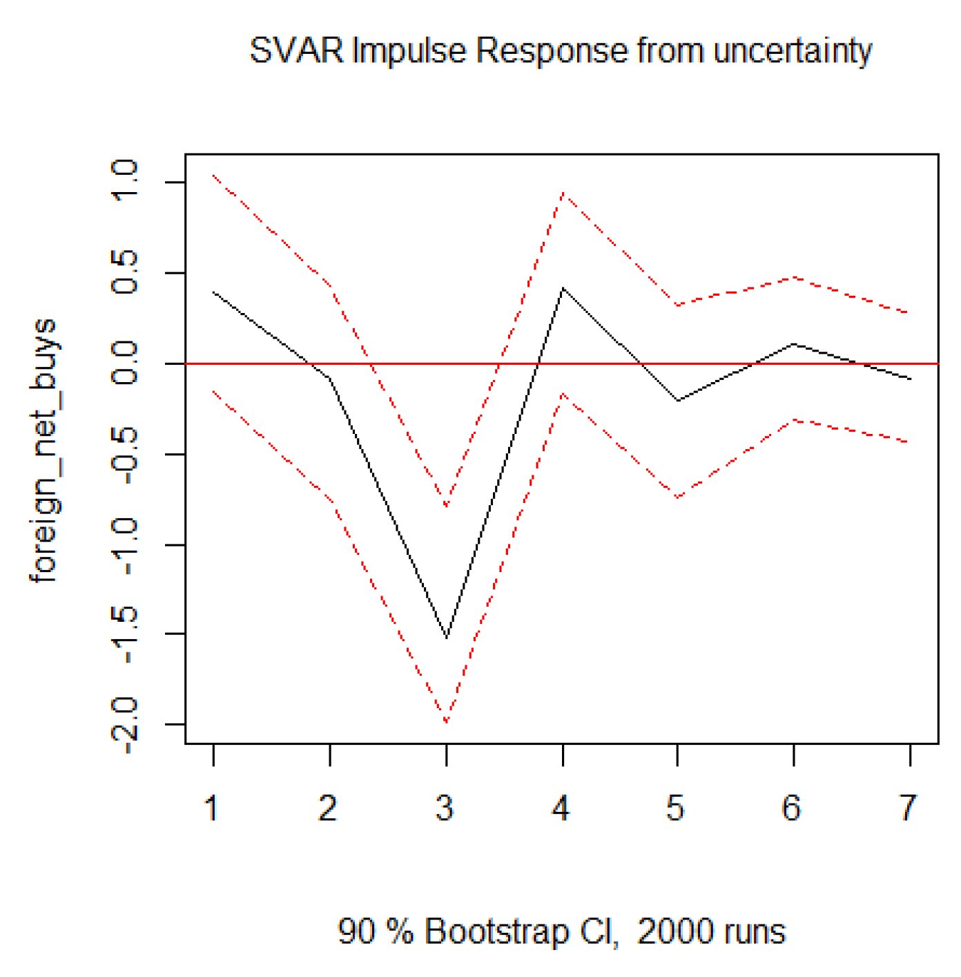
Figure 3.
Forecast Error Variance Decomposition. Note: The figure presents the forecast error variance decomposition for the SVAR estimated using two measures of risk, one measure of uncertainty, changes in exchange rates, and the log of foreigners’ net buys at the aggregate level.
Figure 3.
Forecast Error Variance Decomposition. Note: The figure presents the forecast error variance decomposition for the SVAR estimated using two measures of risk, one measure of uncertainty, changes in exchange rates, and the log of foreigners’ net buys at the aggregate level.
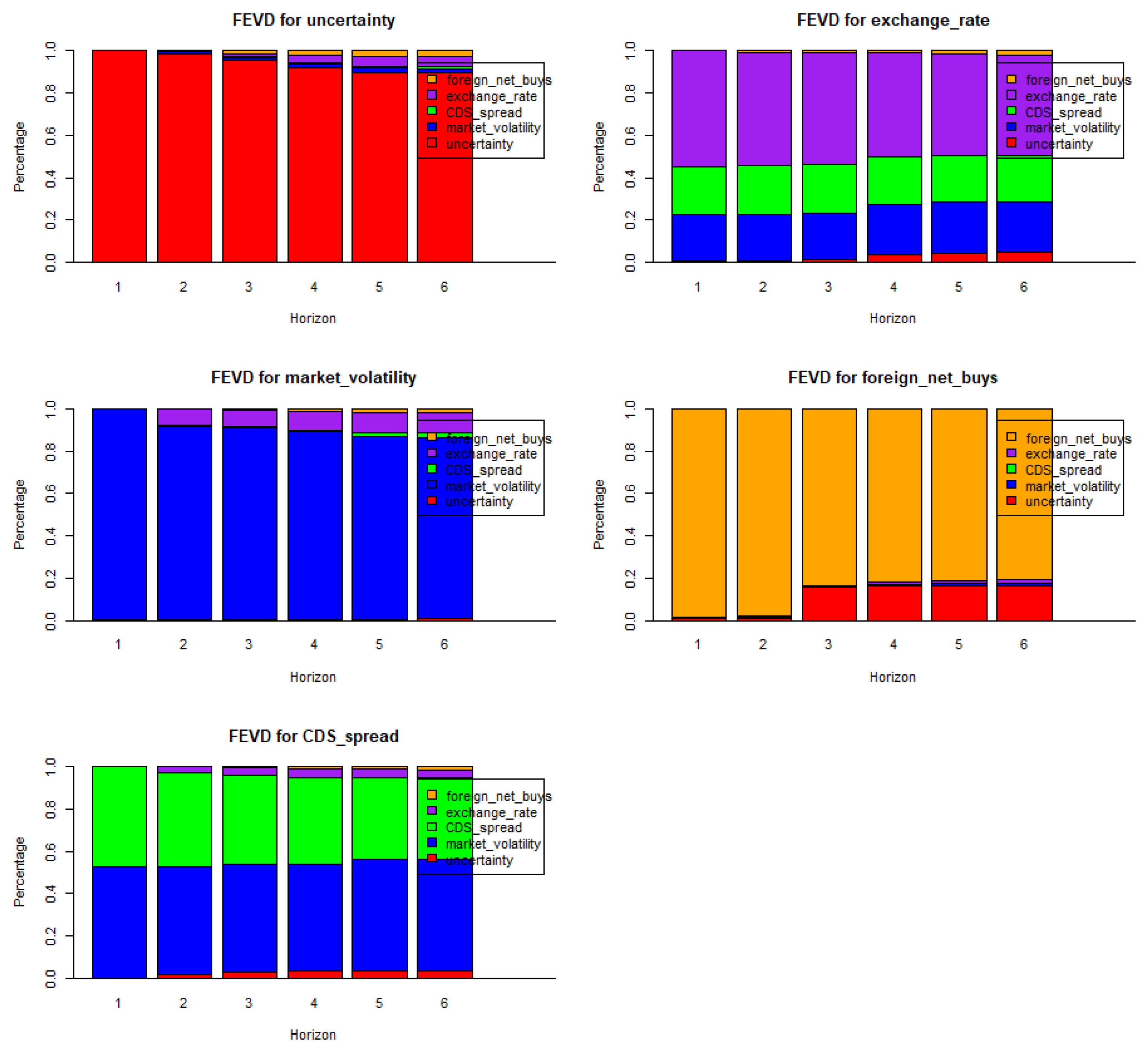
Figure 4.
BSADF Tests. Note: Date-stamping of stock price explosiveness.
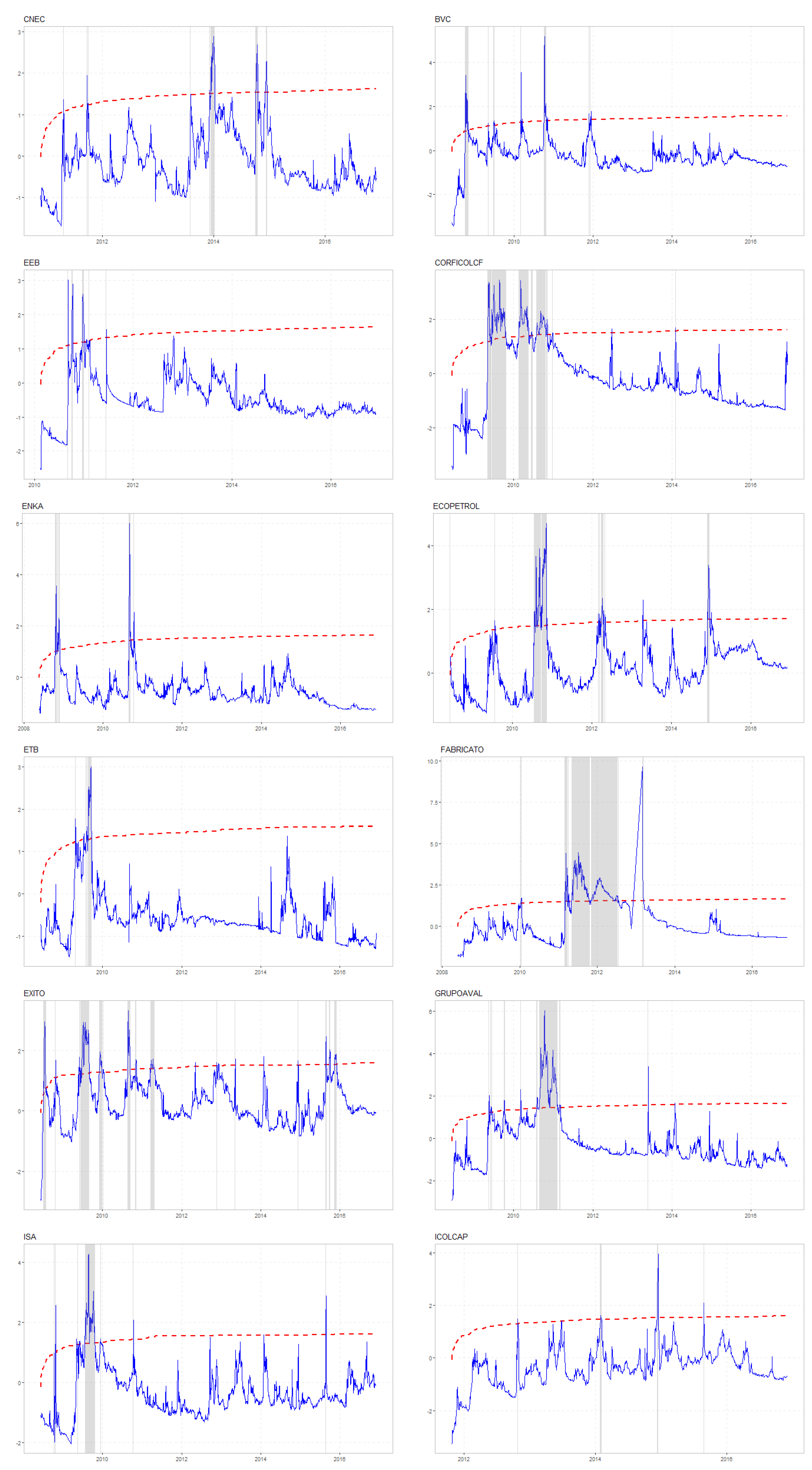
Figure 6.
BSADF Tests (Continuation...). Note: Date-stamping of stock price explosiveness.
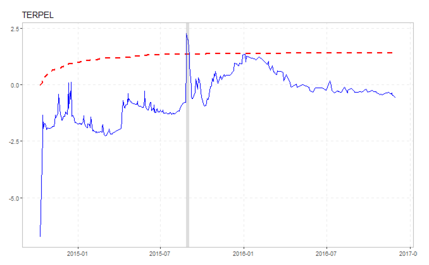

Table 1.
Probability Regression Models
| Panel A | Panel B | |
|---|---|---|
| VIX Index | 1,062*** | 1,112*** |
| (182.899) | (193.1) | |
| Fed Expansion × Local Expansion | 1.891*** | 1.981*** |
| (0.219) | (0.2263) | |
| Exchange Rate | 0.002*** | 0.00179*** |
| (0.0004) | (0.0005) | |
| EPU Index | 0.005*** | 0.005*** |
| (0.002) | (0.001614 ) | |
| Stock Return Volatility | −26.145 | -4.199 |
| (33.887) | (9.335) | |
| Foreigners’ Net Buys | 0.0046*** | 0.00373* |
| (0.002) | (0.002) | |
| CDS Spread | −1.683*** | -1.788*** |
| (0.345) | (0.359) | |
| Montly Stock Return | −0.483 | -0.354 |
| (0.839) | (0.726) | |
| Constant | −7.727*** | – |
| (0.941) | – | |
| Month effects | yes | yes |
| Fixed effects | no | yes |
Note: *p<0.1; **p<0.05; ***p<0.01
Disclaimer/Publisher’s Note: The statements, opinions and data contained in all publications are solely those of the individual author(s) and contributor(s) and not of MDPI and/or the editor(s). MDPI and/or the editor(s) disclaim responsibility for any injury to people or property resulting from any ideas, methods, instructions or products referred to in the content. |
© 2024 by the authors. Licensee MDPI, Basel, Switzerland. This article is an open access article distributed under the terms and conditions of the Creative Commons Attribution (CC BY) license (http://creativecommons.org/licenses/by/4.0/).
Copyright: This open access article is published under a Creative Commons CC BY 4.0 license, which permit the free download, distribution, and reuse, provided that the author and preprint are cited in any reuse.


