
Submitted:
26 July 2023
Posted:
27 July 2023
You are already at the latest version
Preprints on COVID-19 and SARS-CoV-2
Abstract
Inflation in 2021 and 2022 grew much faster than the Federal Reserve expected. The Fed downplayed inflation in 2021 and then increased the federal funds rate by 500 basis points between March 2022 and May 2023. This paper investigates how this unprecedented tightening impacted the stock market. To do so it estimates a fully specified multi-factor model that measures the exposure of 53 assets to Bauer and Swanson (2022) monetary policy surprises over the 1988 to 2019 period. It then uses the monetary policy betas to gauge investors’ beliefs about monetary policy between 2020 and 2023. The results indicate that changing perceptions about monetary policy multiplied uncertainty and stock market volatility.
Keywords:
Monetary policy
; inflation
; stock returns
1. Introduction
News about COVID-19, inflation, and monetary policy
has buffeted the U.S. economy since 2020. As the pandemic emerged, the Federal
Reserve lowered its target for the federal funds rate by 150 basis points in
March 2020. The year-on-year change in the U.S. consumer price index (CPI) then
rose from 1.5% in March 2020 to 8.6% in June 2022. The Fed raised its funds
rate target by 500 basis points in 2022 and 2023. This paper investigates how
monetary policy news has impacted the stock market since the coronavirus crisis
began.
The Fed responded to the pandemic not only by
lowering the funds rate but also by providing forward guidance that interest
rates would remain low, purchasing Treasury and mortgage-backed securities,
lending to Treasury security primary dealers, backstopping money market funds,
and encouraging bank lending and credit extension.1 The government provided
three rounds of stimulus checks. These policies increased demand while negative
shocks associated with the pandemic, value chain disruptions, and the
Russia-Ukraine War restricted supply.
This combination contributed to inflation that
proved higher and more persistent than the Fed expected. At the end of 2020 the
median forecast of Federal Reserve Board members and Federal Reserve Bank
presidents was that the personal consumption expenditures (PCE) price index
would grow by 1.8% between the 2020Q4 and 2021Q4. It actually grew by 5.7%. At
the end of 2021 the median forecast was for the PCE index to grow by 2.6%
between 2021Q4 and 2022Q4. It again grew by 5.7%.2 In November 2021 Fed Chair
Jerome Powell stopped calling inflation transitory and in 2022 the Fed began
aggressively raising the funds rate.
Previous work has investigated the interaction
between monetary policy, inflation, and asset prices after the pandemic.
Gagliardone and Gertler (2023) examined the role of easy monetary policy and
oil shocks in explaining the inflation surge that began in 2021. They employed
a New Keynesian model with oil included as both a consumption good and an input
into production. Their model assumed real wage rigidity and allowed for
unemployment. They derived key parameters by matching the model’s impulse
responses to those obtained from a structural vector autoregression (VAR). They
reported that the inflation that emerged in 2021 arose from a combination of
easy monetary policy (i.e., the delayed response of the Fed to increasing
inflation in 2021) and oil price shocks.
Bernanke and Blanchard (2023) also investigated the
causes of inflation after 2019. They employed a model where nominal wages
depend on labor market slack, prices depend on nominal wages and other input
costs, and expected inflation depends on last period’s expected inflation and
on current inflation. They used their model to impose contemporaneous
restrictions on a structural VAR that they estimated over the 1990Q1-2019Q4
period. They found that commodity price hikes and relative price increases due
to supply shocks led to the inflation that began in 2021. They reported that,
up to 2023, labor market tightness caused only a little inflation.
Eggertsson and Kohn (2023) examined whether the
policy framework (PF) that the Fed implemented in 2020 contributed to the
inflation surge that started in 2021. They noted that the Fed in 2020 adopted
an asymmetric loss function whereby it was less willing to tighten when
employment exceeded its “maximum” level then it was to ease when employment
fell short of this level. They presented narrative evidence that the new PF
caused the Fed to delay tightening as inflation emerged in 2021. They argued
that an earlier response would have promoted financial stability by enabling
the Fed to tighten more gradually.
Chibanea and Kuhanathan (2023), using inflation
swap data, found that the probability of a non-Gaussian jump in U.S. inflation
swaps doubled beginning in the third quarter of 2020. They investigated whether
Fed policy was subsequently able to re-anchor inflation expectations. They used
both an event study of FOMC meetings and short-term interest rates to measure
monetary policy. Their data extended to September 2022. They reported that news
of contractionary monetary policy did not reduce the probability of jumps in
U.S. inflation swaps. They concluded that contractionary monetary policy up to
September 2022 had failed to re-anchor inflation expectations.
Adams et al. (2023) measured financial market
sentiment by applying language processing techniques to Twitter data. They
reported that an unexpected tightening of monetary policy worsens sentiment.
They found that sentiment worsened in September 2021 when Fed communication
pivoted towards a tightening cycle.
Dietrich et al. (2022) employed a daily survey of
consumers’ expectations during the pandemic. They received 60,000 responses.
They reported that consumers expected the pandemic to have a stagflationary
effect. They also found that the pandemic caused huge uncertainty to consumers
about the future path of inflation. Calibrating the consumers’ responses using
a business cycle model, they concluded that better communication by the central
bank to the broader public could have mitigated uncertainty and dampened the
resulting shocks.
Arteta et al. (2022) investigated the factors
affecting U.S. 2-year and 10-year Treasury bond yields in 2022. They employed a
sign-restricted Bayesian VAR using monthly data on 2-year and 10-year Treasury
bond yields, the S&P 500 index, and inflation expectations over the January
1982 to June 2022 period. They reported that changing perceptions of the Fed’s
reaction function, whereby investors inferred the Fed’s changing attitudes to
inflation, explained much of the change in Treasury bond yields in 2022.
Several papers have also highlighted how
uncertainty about macroeconomic variables affects asset returns. Bernanke and
Kuttner (2005), using a VAR and monthly data over the 1973-2002 period, found
that easier monetary policy reduces the risk premium that investors require to
hold stocks. Hanson and Stein (2015), using data on forward interest rates and
monthly data over the 1987-2012 period, presented evidence supporting the
hypothesis that monetary policy affects the term premium on long-term bonds.
Kashyap and Stein (2023), surveying many studies, reported that expansionary
monetary policy lowers risk premia on stocks, Treasury securities, corporate
bonds, and foreign exchange rates.
Chen, Roll, and Ross (CRR) (1986), using monthly
data over the 1958 to 1984 period, found that assets that are harmed by
unexpected increases in inflation must pay higher expected returns. Bekaert,
Wang and Tille (2010), reviewing the literature, found that studies employing
inflation-linked bonds and inflation surveys reported positive risk premia for
assets exposed to inflation. Cieslak and Pflueger (2023), comparing survey
inflation expectation with inflation swap rates over the 2004-2023 period,
reported that inflation risk premia are often negative over the following three
quarters and positive over the following ten years.
This paper investigates how monetary policy has
impacted financial markets since the pandemic began. To do this it first
estimates a multi-factor model including news about monetary policy and other
macroeconomic variables over the 1988 to 2019 period. It then uses assets’
monetary policy betas to examine how investors responded to news about monetary
policy beginning in 2020. If investors believed that monetary policy would
become contractionary, they would sell assets that are harmed by tighter policy
and purchase assets that benefit from tighter policy. This would lower the
prices of assets that are harmed by contractionary monetary policy and raise
the prices of assets that benefit.
The estimated monetary policy betas indicate that
monetary policy matters for many stocks. The results also indicate that
changing perceptions about monetary policy caused large swings in U.S. equity
prices in 2022. Going forward, central bankers should consider how they can
reduce financial market volatility associated with uncertainty about monetary
policy. One way would be to recognize incipient inflation quickly, rather than
waiting until inflation becomes entrenched and then resorting to a monetary
policy sledgehammer. Another way would be to clearly communicate the Fed’s preferences
towards inflation.
The next section presents the data and methodology.
Section 3 presents the results. Section 4 concludes.
2. Data and Methodology
The first goal of this paper is to estimate
monetary policy betas in the context of a fully-specified multi-factor asset
pricing model. Ross (2001) demonstrated that in a multi-factor model an asset’s
expected return equals the return on the risk-free asset plus the inner product
of a vector of assets’ betas to macroeconomic factors with a vector of risk
prices:
where Ei is the ex-ante expected
return on asset i, λ0
is the return on the risk-free asset, βij
is the beta or factor loading of asset i to macroeconomic factor j, and λj is the risk price associated
with factor j. The ex-post realized return equals the sum of the
expected return, a beta-weighted vector of unexpected changes in the
macroeconomic factors, and an error term capturing the effects of idiosyncratic
news:
where Ri is the ex-post realized
return, fj represents news about macroeconomic factor j and εi is a mean-zero error term.
Gallant's (1975) iterated nonlinear seemingly
unrelated regression method (INLSUR) can be used to simultaneously estimate the
factor loadings and the risk prices and to impose the nonlinear cross-equation
restrictions that the intercept terms depend on the risk prices. This technique
delivers consistent estimates of the betas and the risk prices.3 Equation (2) can be stacked and the
model estimated as a system using INLSUR:
Ri -
λ0 is a 1xT
vector where Ri represents
the realized return on asset i and λ0 is the return on the risk-free asset. X(λ,f) is a Txk matrix whose tith
element equals fit + λi . βi is a 1xk
vector measuring asset i's sensit ivity to the macroeconomic factors. εi is an ixT vector,
where by assumption E(ε1, ε2, …, εn) = 0nT, E(ε1, ε2,
…, εn)’(ε1, ε2,
…, εn) = ∑⊗IT, and ∑i,j =
cov((εi,t, εj,t ).
CRR (1986) used observable macroeconomic data (not
latent variables from a dynamic factor model) to measure the common factors.
The factors they employed were the difference in returns between 20-year and
one-month Treasury securities (the horizon premium), the difference in returns
between 20-year corporate bonds and 20-year Treasury bonds (the default
premium), the monthly growth rate in industrial production, unexpected
inflation, and the change in expected inflation. CRR argued that each of these
macroeconomic factors, being either the difference between asset returns or
very noisy, can be treated as innovations. They also argued that, while only
phenomena such as supernovas are truly exogenous, the macroeconomic variables
on the right-hand side can be treated as exogenous relative to the portfolio
returns on the left-hand side.
Thorbecke (2018) reported that the default premium
was not a priced factor. Thus in this paper the default premium is replaced by
an indicator of monetary policy. The other variables are the same ones used by
CRR. Monetary policy is measured using the
surprise monetary policy variable constructed by Bauer and Swanson (B&S)
(2022). They modeled unexpected changes in monetary policy as the first
principal component of the change in the first four Eurodollar futures contracts
over the 30 minutes bracketing Federal Open Market Committee (FOMC)
announcements. Their data extend from January 1988 to December 2019.
Consequently, the sample used here stretches from January 1988 to December
2019.
Unexpected inflation, following Boudoukh,
Richardson, and Whitelaw (1994), is calculated as the residuals from a
regression of the monthly CPI inflation rate on lagged CPI inflation and
current and lagged one-month Treasury bill returns. The change in expected
inflation is also calculated from this model. The data to calculate the
inflation factors and also the horizon premium come from Kroll (2023). Data to
calculate the growth rate of industrial production come from the Federal
Reserve Bank of St. Louis FRED database.
The left-hand side variables include the excess
returns (realized returns minus returns on one-month Treasury bills) on 53
assets. These assets are primarily returns on industry stock portfolios.
However, since Frankel (2008) and others have found that commodities such as gold
and silver can benefit from inflationary news, the returns on gold and silver
are included. This increases the cross-sectional variation in expected returns.
Data on the return on one-month Treasury bills come from Kroll (2023) and data
on the other asset returns come from the Datastream database.
The second goal of this paper is to use the
monetary policy betas to investigate investors’ changing perceptions about
monetary policy beginning in 2020. If investors believe that monetary policy
will become tighter, they will purchase assets that benefit from contractionary
monetary policy (those with larger betas to the B&S variable) and sell
those that are harmed (those with smaller betas to the B&S variable). There
should thus be a positive relationship between asset returns and assets’
B&S betas on months when investors foresee tighter monetary policy.
Similarly, there should be a negative relationship between asset returns and
assets’ B&S betas on months when investors foresee easier monetary policy.
For each month from April 2020 to April 2023, returns on the 53 assets are thus
regressed on the monetary policy betas estimated over the 1988-2019 period.
3. Results
Table 1
presents the risk prices from estimating the multi-factor model. For unexpected
inflation, the value is -0.0011 and the associated probability value is 0.0518.
To understand how this risk price impacts the risk premium, consider the
inflation beta for airlines that equals -3.58. This beta can be viewed as the
quantity of inflation risk associated with the airlines sector. Multiplying the
inflation risk price (-0.0011) by the quantity of inflation risk (-3.58), the
inflation risk premium associated with airlines is 0.0038. This implies that
the required return to hold airline stocks is raised by 0.38% per month because
airline stocks perform badly when inflation increases. On the other hand, the
estimated inflation beta for silver is 3.34. Multiplying the risk price by the
quantity of inflation risk, the risk premium associated with silver is -0.0036.
This implies that the required return to hold silver decreases by 0.36% per
month because silver does well when inflation increases.
Bekaert, Wang and Tille (2010) reported positive risk premia for assets that are harmed by higher inflation. Cieslak and Pflueger (2023), on the other hand, found that inflation risk premia are often negative over the following three quarters. The results here are consistent with Bekaert et al.’s findings that assets exposed to inflation must pay a positive increment to their required returns.
For the horizon premium, the risk price in Table 1 equals -0.0092 and is statistically significant at the 1% level. The horizon premium measures the difference in returns between 20-year and one-month Treasury securities. It is closely related to the spread between long-term and short-term interest rates. A decrease in this spread helps predict a recession (see, e.g., Hornstein, 2022). A decrease in the long-term interest rate would cause a capital gain for those holding long-term bonds and thus increase the horizon premium. So an increase in the horizon premium is associated with a decrease in the long/short interest rate spread.
For sectors more exposed to decreases in the interest rate spread (those with negative betas to the horizon premium), the risk price in Table 1 implies that they would have to pay higher expected returns. For instance, for the automobile sector the horizon premium beta equals -0.543. Automobile stocks would thus have to pay a risk premium of -0.0092 x -0.543= 0.0050. Thus auto stocks would have to pay a positive premium of 0.50% per month to compensate for their exposure to the automobiles sector. On the other hand, the electricity sector is less cyclically sensitive and its horizon premium beta equals 0.326. Electricity stocks would thus have a required return of 0.30% less per month because they do well when the horizon premium increases.
The risk price associated with industrial production is also statistically significant but the risk prices associated with the change in expected inflation and with monetary policy are not. The insignificant coefficient on the monetary policy risk price does not indicate that monetary policy does not affect risk premia. Economists have long highlighted the possibility of time-varying risk premium associated with uncertainty about monetary policy (see, e.g., Campbell, 1995). If this is true, the average risk price reported in Table 1 could be insignificant because it reflects both periods when the risk price has been positive and periods when it has been negative.
While the risk price associated with monetary policy is not significantly different from zero, many of the monetary policy betas are. These are presented in Table 2.4 Of the 53 assets, 22 have statistically significant exposures at the 1% level, 13 more have statistically significant exposures at the 5% level, and five more at the 10% level. These results indicate that contractionary monetary policy harms many assets. For those with statistically significant exposures to monetary policy, a one-standard deviation B&S monetary policy surprise would reduce returns on average by 1%.
A wide cross section of assets in Table 2 is harmed by contractionary monetary policy. The ones that are not tend to be necessities and stocks that are not cyclically sensitive such as utilities, food producers, consumer staples, and drug retailers.
To understand how investors interpreted monetary policy actions after the pandemic, Figure 1 plots all of the months between April 2020 and April 2023 when there was a statistically significant relationship at at least the 10% level between the returns on the 53 assets and their B&S monetary policy betas. To facilitate interpretation, the regression coefficient is multiplied by the average of the 40 statistically significant monetary policy betas in Table 2. Since the average of the 40 beta coefficients is negative, the product of this average and the regression coefficient is positive when investors expect Fed policy to become easier and negative when they foresee tighter policy. The coefficients in Figure 1 show how investors’ responses to monetary policy news affected an asset with an average degree of exposure to contractionary monetary policy. Figure 1 also plots the year-on-year increase in the Fed’s preferred inflation measure, the PCE price index.
The figure shows that investors in April, May, June, and July 2020 expected the path of monetary policy to become looser. Easier monetary policy seemed appropriate at this time as the economy faced headwinds from a once in a lifetime pandemic, as nonfarm employment between March and July 2020 fell by 52 standard deviations, and as the PCE inflation rate was below 1%.
The figure also shows that in 2021 the PCE inflation rate rose from 1.5% to 6.1%, reaching its highest level in 40 years. As inflation soared in 2021, however, investors did not foresee tighter monetary policy. They even priced in easier monetary policy in May 2021. While Adams et al. (2021) reported that the Fed’s communication pivot towards a tightening cycle worsened sentiment in September 2021, there is no evidence in Figure 1 that investors bid down stock prices in September in response to this.
As inflation increased by another 200 basis points in 2022, the Fed reacted violently. Beginning in March 2022, it increased its federal funds rate target by 500 basis points. Figure 1 shows that investors priced in contractionary shifts in the course of policy in January, April, May and June. One thing that is striking in Figure 1 is the magnitude of the stock market response. For instance, in June 2022, anticipations of contractionary monetary policy pushed down returns on assets with average exposure to monetary policy by 11.9%. For the asset most exposed to monetary policy in Table 2, contractionary monetary policy pushed down returns by more than 24%.
The second thing that is striking in Figure 1 is how investors’ perceptions in 2022 changed from month to month. Until June 2022 they kept betting on monetary policy becoming tighter than they had anticipated. In July they foresaw easier monetary policy, in August they expected tighter monetary policy again, and in October and November they priced in easier policy. The beta values in Table 2 indicate that monetary policy exerts important effects on many stocks, and during the drastic tightening in 2022 investors focused on how these stocks would be affected by changes in the future course of monetary policy. They bid stock prices up and down several times in response to changing monetary policy perceptions.
Figure 2 shows that there was a close relationship in 2022 between changes in returns associated with monetary policy and returns on the S&P 500 aggregate index of large companies. As changing perceptions of monetary policy caused large swings in stocks, the S&P 500 moved back and forth in the same direction.
Figure 3 examines the stock market responses during the volatile period from April to August 2022 using daily data. It plots changes in returns associated with monetary policy for all of the business days between 1 April 2022 and 31 August 2022 when there was a statistically significant relationship at at least the 5% level between the returns on the 53 assets and their B&S monetary policy betas. The figure indicates that, of the 109 business days over this period, there was a systematic reaction to monetary policy news on 46 days. Thus investors priced in changes in the future path of monetary policy on almost half of the days. There was also a close correlation between aggregate stock returns and changes in returns on an asset with average exposure to monetary policy in Figure 3. Regressing the former on the latter yields a coefficient of 0.92 and a t-statistic, calculated using HAC standard errors, of 8.84.5
Many of the dates plotted in Figure 3 correspond to dates when there was important news related to monetary policy. For instance, the 2.5% drop in Figure 3 on April 6 occurred on the day when the minutes from the previous FOMC meeting indicated that many officials had wanted a larger funds rate increase in March 2022 (Megaw et al., 2022). The 1.4% drop on May 11 and the 1.9% drop on June 10 occurred on days when news revealed that U.S. consumer prices rose more than expected in the previous month (Smith, 2022a and 2022b). The 1.5% increase on July 27 occurred when Fed Chair Powell said that the Fed would likely slow the pace of funds rate increases (Martin, 2022). The 1.1% decrease on August 26 occurred when Powell gave a hawkish inflation speech (Smith and Platt, 2022).
Figure 2 and Figure 3 indicate that news about monetary policy contributed to large swings in stock returns. As the Fed in 2022 began what Eggertsson and Kohn (2023) called an unprecedented increase in the federal funds rate, investors drove stock prices up and down in response to changing perceptions about the future path of monetary policy. Arteta et al. (2022) found that much of the Fed’s impact on financial markets in 2022 occurred because investors kept updating their beliefs about the Fed’s preferences towards inflation. As the Fed pursued drastic tightening it sewed confusion and multiplied volatility in the U.S. stock market, one of the world’s most important financial markets.
Figure 1 indicates that investors priced in easier monetary policy in January 2023. At this time, though, the measure of monetary policy uncertainty constructed using the methods of Baker et al. (2016) reached the fifth highest level over the 460 months for which data are available.6 Complex uncertainty concerning the future path of monetary policy thus continued into 2023. By increasing uncertainty and spawning volatility, the Fed made firms more hesitant to invest (see. e.g., Bloom et al., 2007).
4. Conclusion
The Federal Reserve was slow to recognize that inflation after the pandemic would persist. It did not tighten policy until 2022 after the PCE inflation rate reached its highest level in more than 40 years. It then undertook an unprecedented tightening, raising the federal funds rate by 500 basis points in 15 months. These actions multiplied stock market volatility. They also contributed to 26% losses in both long-term corporate and Treasury bonds in 2022. This is by far the worst bond market performance over the 97 years that Kroll (2023) provides data. Rajan (2023) noted that the Fed’s highly expansionary policies before 2022 generated financial instability by pushing investors into riskier, higher-yielding assets that performed badly when the Fed tightened.
What can central bankers learn from this experience? Huw Pill, the chief economist at the Bank of England, noted that the economic models they used to forecast inflation after the pandemic were estimated over periods when shocks were less extreme (Giles, 2023). Regression techniques are only valid locally, and are unreliable when extrapolated outside of the range of observed data.7 Policymakers’ perspectives were also formed during periods when inflation was quiescent, and this contributed to misinterpreting the inflationary shocks that began in 2021 as transitory.
Faced with extreme or unusual events, policymakers should learn from historical episodes, dialogue with others whose worldviews differ from theirs, and communicate well. History does not repeat itself but it rhymes. Studying similar events in the past can shed light on how shocks will impact inflation and other key variables in the present.
Listening to people with different perspectives can also be beneficial. Granovetter (1973) showed that people who work closely together tend to think alike. When the economy faces unusual shocks, it is salutary for FOMC members to exchange ideas with others with whom they share only “weak ties.” This can expose policymakers to new ideas, enable them to reevaluate their own implicit models, and help them to understand why their forecasts might prove wrong.
Adams et al. (2023) found that Fed communication pivoted towards a tightening cycle in 2021. However, the results reported here indicate that markets only began pricing in monetary tightening in 2022. Eggertsson and Kohn (2023) observed that many were uncertain of the Fed’s intentions. Dietrich et al. (2022) found that better communication by the central bank to the public could have mitigated uncertainty. Arteta et al. (2022) reported that changing perceptions about the Fed’s preferences towards inflation explained much of the movement in asset prices in 2022 and concluded that proper communication that clarified the Fed’s reaction function could have reduced adverse spillovers. Improved communication could thus have helped to attenuate the wild swings in stock prices that arose because of uncertainty about monetary policy.
The economy will face challenging shocks going forward. It may respond differently to these than it has to shocks in the past. Central bankers need to be nimble and pragmatic and skillful at updating their beliefs about how the world works.
Funding
This research received no external funding.
| 1 | See Milstein and Wessel (2021) for a discussion of monetary policy during the pandemic. |
| 2 | These data come from the statements accompanying Federal Open Market Committee meetings (https://www.federalreserve.gov/monetarypolicy/fomccalendars.htm) and from the Federal Reserve Bank of St. Louis FRED database. |
| 3 | See McElroy and Burmeister (1988). |
| 4 | Betas for the other macroeconomic factors are available on request. |
| 5 | HAC standard errors refers to heteroscedasticity and autocorrelation consistent standard errors. |
| 6 | These data are available at: http://www.policyuncertainty.com/ . |
| 7 | Furman (2023) also highlights the pitfalls of using a linear model to evaluate the impact of large shocks. |
Conflicts of Interest
The author declares no conflict of interest.
References
- Adams, T.; Ajello, A.; Silva, D.; Vazquez-Grande, F. 2023. “More than Words: Twitter Chatter and Financial Market Sentiment.” Working Paper No. 2023-034, Finance and Economics Discussion Series, Board of Governors of the Federal Reserve System.
- Arteta, C.; Kamin, S.; Ruch, F. U. 2022. “How Do Rising U.S. Interest Rates Affect Emerging and Developing Economies? It Depends.” Policy Research Working Paper 10258, World Bank.
- Baker, S.; Bloom, N.; Davis, S. Measuring Economic Policy Uncertainty. Quarterly Journal of Economics 2016, 131, 1593–1636. [Google Scholar] [CrossRef]
- Bauer, M.; Swanson, E. 2022. “A Reassessment of Monetary Policy Surprises and High-Frequency Identification.” In NBER Macroeconomics Annual 2022, Vol. 37, ed. M. Eichenbaum, E. Hurst, and V. Ramey. Chicago: University of Chicago Press.
- Bekaert, G.; Wang, X.; Tille, C. Inflation Risk and the Inflation Risk Premium. Economic Policy 2010, 25, 755–806. [Google Scholar] [CrossRef]
- Bernanke, B.; Kuttner, K. What Explains the Stock Market's Reaction to Federal Reserve Policy? Journal of Finance 2005, 60, 1221–1257. [Google Scholar] [CrossRef]
- Bernanke, B.; Blanchard, O. 2023. “What Caused the U.S. Pandemic-Era Inflation?” Presentation at Hutchins Center, Brookings Institution, 23 May. Available at: https://www.brookings.edu/wp-content/uploads/2023/04/Bernanke-Blanchard-conference-draft_5.23.23.pdf.
- Boudoukh, J.; Richardson, M.; Whitelaw, R. Industry Returns and the Fisher Effect. Journal of Finance 1994, 44, 1595–1615. [Google Scholar] [CrossRef]
- Campbell, J.Y. Some Lessons from the Yield Curve. Journal of Economic Perspectives 1995, 9, 129–152. [Google Scholar] [CrossRef]
- Chen, N.; Roll, R.; Ross, S. Economic Forces and the Stock Market. Journal of Business 1986, 59, 383–403. [Google Scholar] [CrossRef]
- Chibane, M.; Kuhanathan, A. Is The Fed Failing To Re-Anchor Expectations? An Analysis of Jumps in Inflation Swaps. Finance Research Letters forthcoming. 2023. [Google Scholar] [CrossRef]
- Cieslak, A.; Pflueger, C. 2023. “Inflation and Asset Returns.” Working Paper No. 30982, National Bureau of Economic Research.
- Dietrich, A.; Kuester, K.; Müller, G.; Schoenle, R. News and Uncertainty about COVID-19: Survey Evidence and Short-run Economic Impact. Journal of Monetary Economics 2022, 129, S35–S51. [Google Scholar] [CrossRef] [PubMed]
- Eggertsson, G.; Kohn, D. 2023. “The Inflation Surge of the 2020s: The Role of Monetary Policy.” Presentation at Hutchins Center, Brookings Institution, 23 May. Available at: https://www.brookings.edu/wp-content/uploads/2023/04/Eggertsson-Kohn-conference-draft_5.23.23.pdf.
- Frankel, J. 2008. “The Effect of Monetary Policy on Real Commodity Prices.” In Asset Prices and Monetary Policy, ed. J. Y. Campbell, 291–333, Chicago: University of Chicago Press.
- Furman, J. 2023. “Inflation: A Series of Unfortunate Events vs. Original Sin.” Presentation at Hutchins Center, Brookings Institution, 23 May. Available at: https://www.brookings.edu/wp-content/uploads/2023/04/20230523-Hutchins-Inflation-Comment-v2.pdf .
- Gagliardone, L.; Gertler, M. 2023. “Oil Prices, Monetary Policy and Inflation Surges.” Working Paper No. 31263, National Bureau of Economic Research.
- Gallant, A. Nonlinear Regression. The American Statistician 1975, 29, 73–81. [Google Scholar]
- Giles, C. Bank of England Admits ‘Very Big Lessons to Learn’ over Failure to Forecast Rise in Inflation. Financial Times, 24 May 2023. [Google Scholar]
- Granovetter, M. The Strength of Weak Ties. American Journal of Sociology 1973, 78, 1360–1380. [Google Scholar] [CrossRef]
- Hanson, S.; Stein, J. Monetary Policy and Long-Term Real Rates. Journal of Financial Economics 2015, 115, 429–448. [Google Scholar] [CrossRef]
- Hornstein, A. 2022. “Recession Predictors: An Evaluation.” Economic Brief No. 22–30. Federal Reserve Bank of Richmond.
- Kashyap, A.; Stein, J. Monetary Policy When the Central Bank Shapes Financial-Market Sentiment. Journal of Economic Perspectives 2023, 37, 53–76. [Google Scholar] [CrossRef]
- Kroll. 2023 SBBI Yearbook; Kroll: New York, 2023. [Google Scholar]
- Martin, K. Investors Clutch at Reasons to Hope. Financial Times, 29 July 2022. [Google Scholar]
- McElroy, M.; Burmeister, E. 1988. Arbitrage Pricing Theory as a Restricted Nonlinear.
- Megaw, N.; Rovnik, N.; Langley, W. US Stocks End Lower after Fed Minutes Point to Tighter Monetary Policy. Financial Times, 7 April 2022. [Google Scholar]
- Milstein, D.; Wessel, D. What Did the Fed Do in Response to the COVID-19 Crisis? Brookings Weblog. 17 December 2021. Available online: https://www.brookings.edu/research/fed-response-to-covid19/.
- McElroy, Marjorie B.; Burmeister, Edwin. Arbitrage pricing theory as a restricted nonlinear multivariate regression model iterated nonlinear seemingly unrelated regression estimates. Journal of Business & Economic Statistics 1988, 6, 29–42. [Google Scholar]
- Bloom, N.; Bond, S.; Van Reenen, J. Uncertainty and Investment Dynamics. The Review of Economic Studies 2007, 74, 391–415. [Google Scholar] [CrossRef]
- Rajan, R. Not Buying Central Banks’ Favorite Excuse. Project Syndicate Weblog, 26 May 2023. [Google Scholar]
- Ross, S. 2001. Finance. In The New Palgrave Dictionary of Money and Finance, ed. P. Newman, M. Milgate, and J. Eatwell, 1–34, London: Macmillan Press.
- Smith, C. US Inflation Resumes Rapid Rise by Accelerating in May. Financial Times, 11 June 2022a. [Google Scholar]
- Smith, C. US Inflation Stays at 40-year High, Defying Expectations of Bigger Drop. Financial Times, 12 May 2022b. [Google Scholar]
- Smith, C.; Platt, E. Jay Powell Says Fed Will ‘Keep at It” in Hawkish Inflation Speech. Financial Times, 27 August 2022. [Google Scholar]
- Thorbecke, W. The Effect of the Fed's Large-scale Asset Purchases on Inflation Expectations. Southern Economic Journal 2018, 85, 407–423. [Google Scholar] [CrossRef]
Figure 1.
The Personal Consumption Expenditures (PCE) Inflation Rate and the Monthly Change in Returns Associated with Exposure to Monetary Policy. Note: The figure presents the personal consumption expenditures (PCE) inflation rate and the change in returns associated with monetary policy. To calculate the change in returns associated with monetary policy, assets’ monetary policy betas are estimated. The betas are obtained from an iterated nonlinear seemingly unrelated regression (INLSUR) of returns on 53 assets (minus the return on one-month Treasury bills) on the Bauer and Swanson (B&S) (2022) measure of Fed policy surprises, the difference in returns between 20-year and one-month Treasury securities, the monthly growth rate in industrial production, unexpected inflation, and the change in expected inflation. The B&S measure is constructed so that an increase represents a contractionary monetary policy surprise. If investors believe that monetary policy will tighten, they will purchase assets that benefit from contractionary monetary policy (those with larger betas to the B&S variable) and sell assets that are harmed by contractionary monetary policy (those with smaller betas to the B&S variable). There should thus be a positive relationship between asset returns and assets’ B&S betas on months when investors foresee monetary policy tightening. For each month between April 2020 and April 2023, returns on the 53 assets are thus regressed on the assets’ monetary policy betas. To facilitate interpretation, the resulting regression coefficient is multiplied by the average beta coefficient for the 40 assets from the INLSUR regression that exhibited statistically significant exposures to contractionary monetary policy. The change in returns associated with monetary policy in the figure thus represents the change for an asset with an average level of exposure to contractionary monetary policy. Since the average B&S beta coefficient is negative, positive values in Figure 1 indicate that investors expect easier policy and negative values that they foresee tighter policy. The figure only reports months when there is a statistically significant relationship (at at least the 10 percent level) between returns on the 53 assets and the assets’ monetary policy betas.
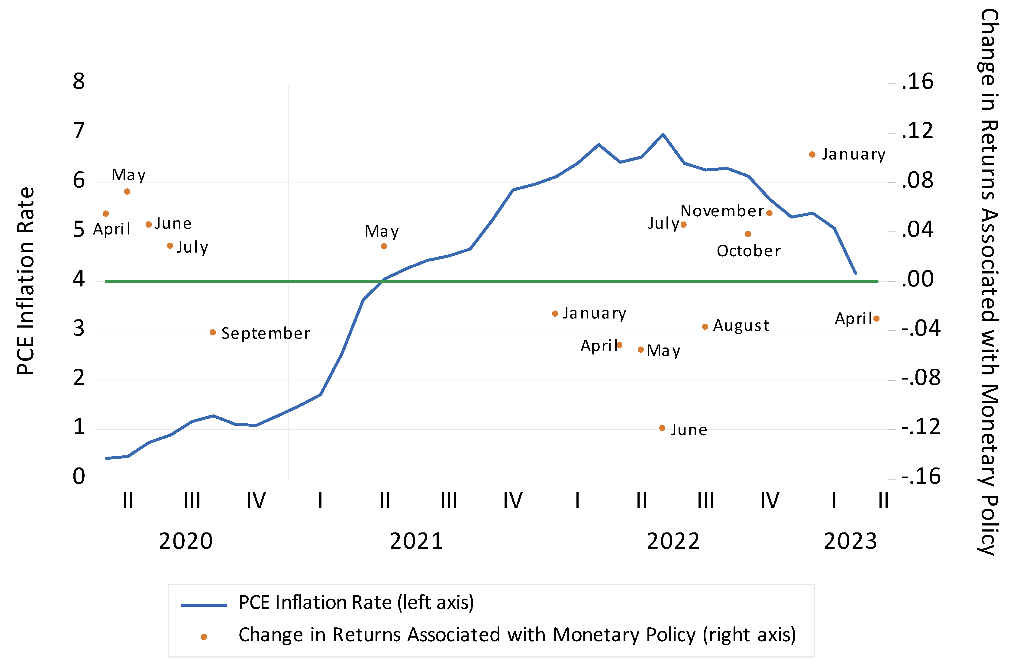
Figure 2.
The Return on the Standard and Poor’s 500 and the Monthly Change in Returns Associated with Exposure to Monetary Policy in 2022. Note: The figure presents the monthly returns on the Standard & Poor’s 500 index of 500 of the largest companies in the U.S. and the change in returns associated with monetary policy. To calculate the change in returns associated with monetary policy, assets’ monetary policy betas are estimated. The betas are obtained from an iterated nonlinear seemingly unrelated regression (INLSUR) of returns on 53 assets (minus the return on one-month Treasury bills) on the Bauer and Swanson (B&S) (2022) measure of Fed policy surprises, the difference in returns between 20-year and one-month Treasury securities, the monthly growth rate in industrial production, unexpected inflation, and the change in expected inflation. The B&S measure is constructed so that an increase represents a contractionary monetary policy surprise. If investors believe that monetary policy will tighten, they will purchase assets that benefit from contractionary monetary policy (those with larger betas to the B&S variable) and sell assets that are harmed by contractionary monetary policy (those with smaller betas to the B&S variable). There should thus be a positive relationship between asset returns and assets’ B&S betas on months when investors foresee monetary policy tightening. For each month between April 2020 and April 2023, returns on the 53 assets are thus regressed on theassets’ monetary policy betas. To facilitate interpretation, the resulting regression coefficient is multiplied by the average beta coefficient for the 40 assets from the INLSUR regression that exhibited statistically significant exposures to contractionary monetary policy. The change in returns associated with monetary policy in the figure thus represents the change for an asset with an average level of exposure to contractionary monetary policy. Since the average B&S beta coefficient is negative, positive values in Figure 2 indicate that investors expect easier policy and negative values that they foresee tighter policy. The figure only reports months when there is a statistically significant relationship (at at least the 10 percent level) between returns on the 53 assets and the assets’ monetary policy betas.
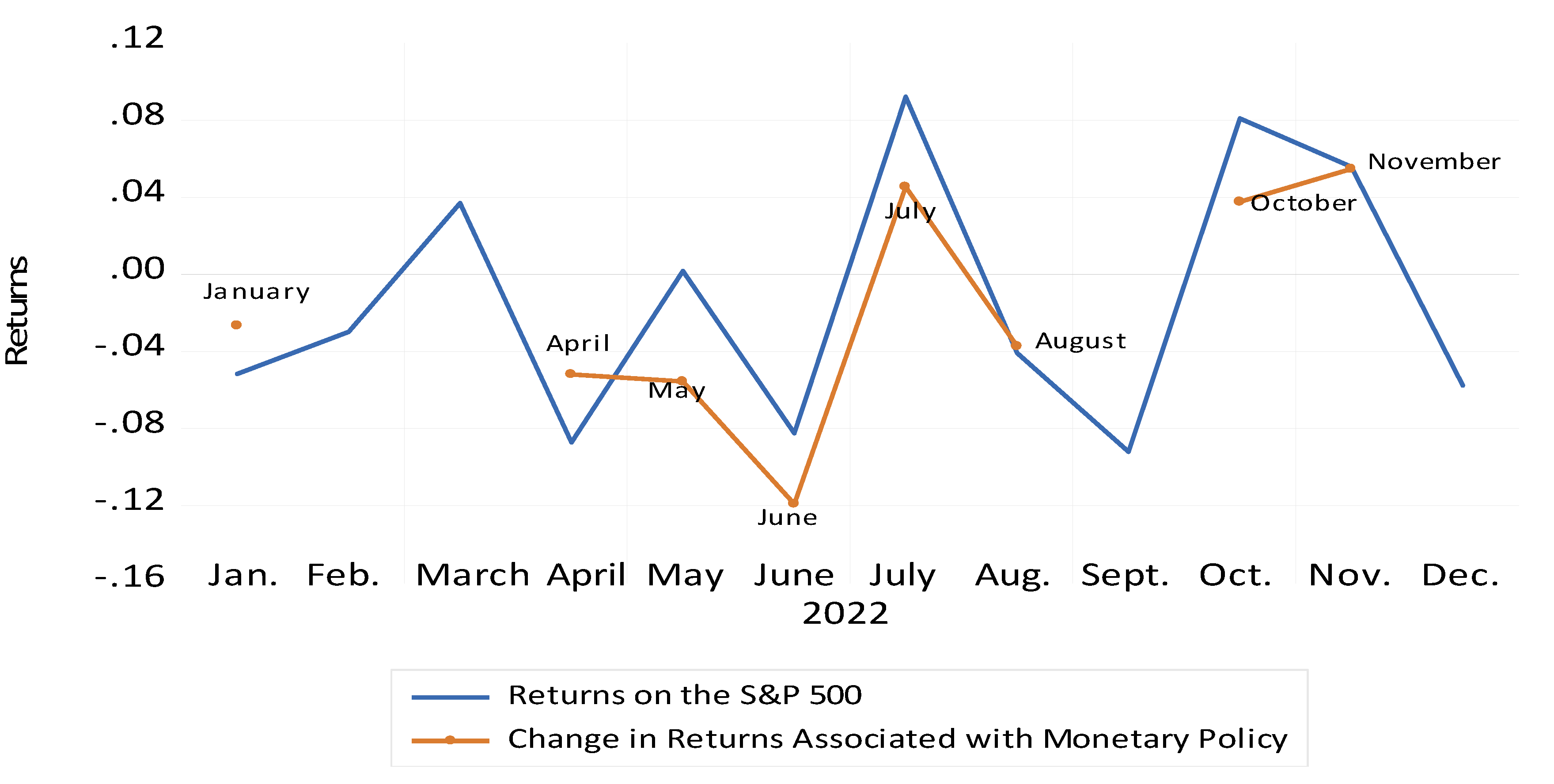
Figure 3.
The Daily Change in Returns Associated with Exposure to Monetary Policy between 1 April and 31 August 2022. Note: The figure presents the daily change in returns associated with monetary policy. To calculate the change in returns associated with monetary policy, assets’ monetary policy betas are estimated. The betas are obtained from an iterated nonlinear seemingly unrelated regression (INLSUR) of returns on 53 assets (minus the return on one-month Treasury bills) on the Bauer and Swanson (B&S) (2022) measure of Fed policy surprises, the difference in returns between 20-year and one-month Treasury securities, the monthly growth rate in industrial production, unexpected inflation, and the change in expected inflation. The B&S measure is constructed so that an increase represents a contractionary monetary policy surprise. If investors believe that monetary policy will tighten, they will purchase assets that benefit from contractionary monetary policy (those with larger betas to the B&S variable) and sell those that are harmed by contractionary monetary policy (those with smaller betas to the B&S variable). There should thus be a positive relationship between asset returns and assets’ B&S betas on days when investors foresee tighter monetary policy. For each business day between 1 April 2022 and 31 August 2022, returns on the 53 assets are thus regressed on the assets’ monetary policy betas. To facilitate interpretation, the regression coefficient is multiplied by the average beta coefficient for the 40 assets from the INLSUR regression that exhibited statistically significant exposures to contractionary monetary policy. The change in returns associated with monetary policy in the figure thus represents the change for an asset with an average level of exposure to contractionary monetary policy. Since the average B&S beta coefficient is negative, positive values in Figure 3 indicate that investors expect easier policy and negative values that they foresee tighter policy. The figure only reports months when there is a statistically significant relationship (at at least the 5 percent level) between returns on the 53 assets and the assets’ monetary policy betas.
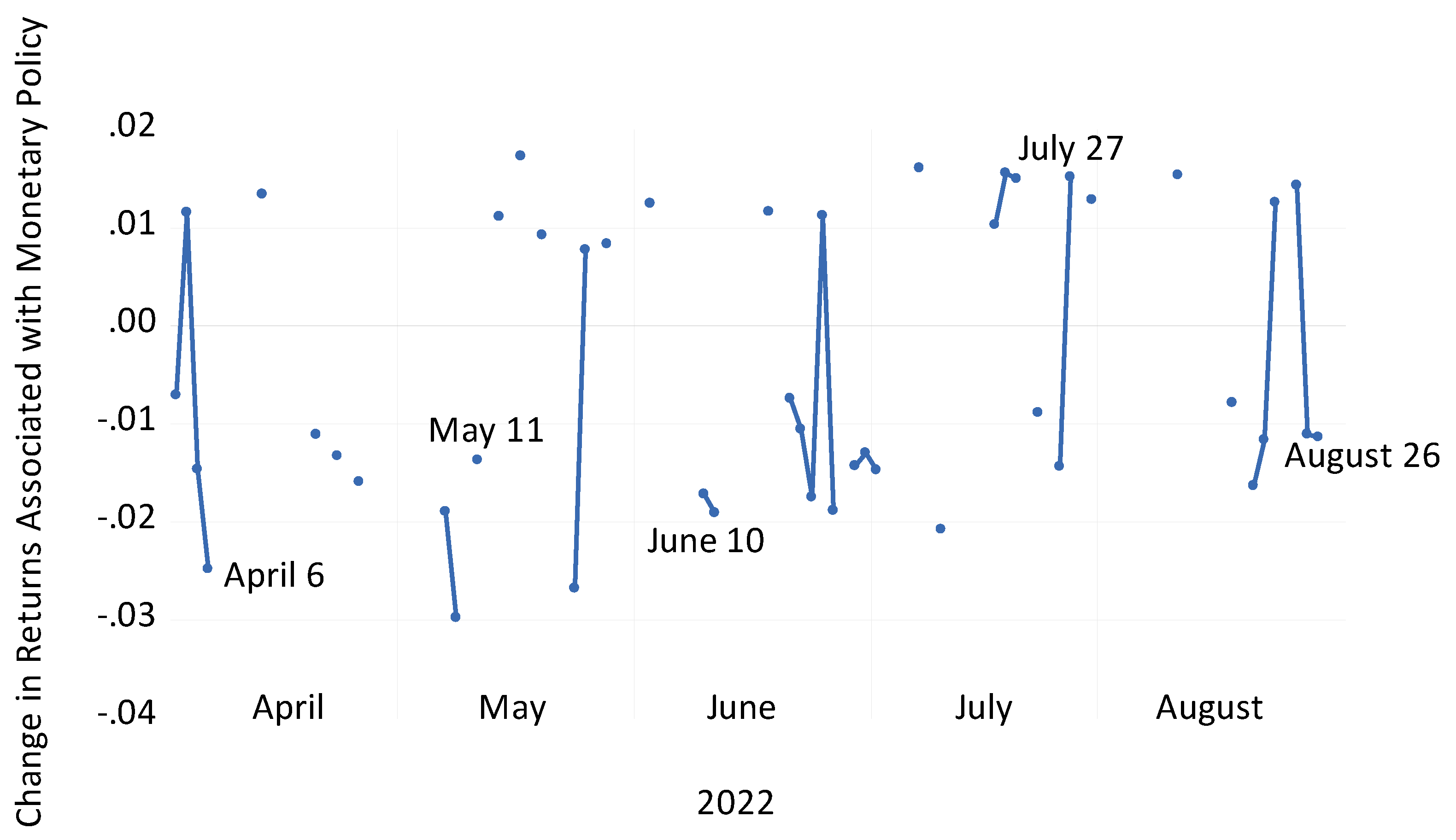

Table 1.
Iterated Nonlinear Seemingly Unrelated Regression Estimates of the Risk Prices Associated with Macroeconomic Factors.
Table 1.
Iterated Nonlinear Seemingly Unrelated Regression Estimates of the Risk Prices Associated with Macroeconomic Factors.
| (1) | (2) |
|---|---|
| Macroeconomic Factor | Risk Price |
| Unexpected Inflation | -0.0011* (0.0006) |
| Horizon Premium | -0.0092*** (0.0033) |
| Industrial Production Growth | -0.0069*** (0.0014) |
| Change in Expected Inflation | -0.0002 (0.0003) |
| Monetary Policy | -0.0068 (0.0094) |
Note: The table presents iterated nonlinear seemingly unrelated regression estimates of risk prices from a multi-factor model including returns on 53 assets (minus the return on one-month Treasury bills) on the left-hand side and the difference between returns on 20-year and one-month Treasury securities, the Bauer and Swanson (B&S) (2022) measure of Fed policy surprises, the monthly growth rate in industrial production, unexpected inflation, and the change in expected inflation on the right-hand side. The B&S measure is constructed so that an increase represents a contractionary monetary policy surprise. Unexpected inflation is calculated as the residuals from a regression of the consumer price index inflation rate on lagged inflation and current and lagged Treasury bill returns. The change in expected inflation is also calculated from this model. The sample extends from January 1988 to December 2019. ***(*) denotes significance at the 1% (10%) level.
Table 2.
Iterated Nonlinear Seemingly Unrelated Regression Estimates of Assets’ Sensitivities to Bauer and Swanson (2022) Fed Policy Surprises.
Table 2.
Iterated Nonlinear Seemingly Unrelated Regression Estimates of Assets’ Sensitivities to Bauer and Swanson (2022) Fed Policy Surprises.
| (1) | (2) | (3) |
|---|---|---|
| Asset | Monetary Policy Beta | Standard Error |
| Aerospace/Defense | -0.160*** | 0.049 |
| Aerospace | -0.159*** | 0.055 |
| Airlines | -0.223*** | 0.079 |
| Aluminum | -0.285*** | 0.092 |
| Apparel Retail | -0.183** | 0.074 |
| Auto & Parts | -0.149** | 0.069 |
| Auto Parts | -0.141** | 0.060 |
| Automobiles | -0.127 | 0.087 |
| Basic Materials | -0.206*** | 0.054 |
| Basic Resources | -0.252*** | 0.068 |
| Beverages | -0.049 | 0.043 |
| Broadcast & Entertainment | -0.168** | 0.069 |
| Brewers | -0.051 | 0.052 |
| Building Materials/Fixtures | -0.101* | 0.059 |
| Business Supply Services | -0.207*** | 0.047 |
| Chemicals | -0.184*** | 0.05 |
| Clothing & Accessories | -0.232*** | 0.066 |
| Commercial Vehicles/Trucks | -0.236*** | 0.069 |
| Computer Hardware | -0.194*** | 0.071 |
| Computer Services | -0.157*** | 0.05 |
| Construction & Materials | -0.144** | 0.058 |
| Consumer Electricity | -0.013 | 0.038 |
| Consumer Discretionary | -0.181*** | 0.044 |
| Consumer Finance | -0.124** | 0.062 |
| Consumer Goods | -0.158*** | 0.044 |
| Consumer Staples | -0.068* | 0.036 |
| Consumer Services | -0.197*** | 0.043 |
| Container & Packaging | -0.218*** | 0.052 |
| Defense | -0.166*** | 0.053 |
| Distillers & Vintners | -0.040 | 0.056 |
| Diversified Industrials | -0.126** | 0.053 |
| Drug Retailers | -0.072 | 0.058 |
| Durable Household Products | -0.165** | 0.074 |
| Electronic Components & Equipment | -0.233*** | 0.057 |
| Electricity | -0.014 | 0.038 |
| Electronic & Electrical Equipment | -0.247*** | 0.057 |
| Food & Drug Retail | -0.103** | 0.04254 |
| Food Producers | -0.050 | 0.037 |
| Food Retailers & Wholesalers | -0.080* | 0.048 |
| Financial Services | -0.148*** | 0.056 |
| Financials | -0.114** | 0.051 |
| Gold Bullion | -0.036 | 0.04 |
| Gold Mining (Americas) | -0.142 | 0.09 |
| Gold Mining (Australasia) | -0.347*** | 0.1 |
| Gold Mining (World) | -0.186** | 0.086 |
| Health Care | -0.080** | 0.037 |
| Oil & Gas | -0.087* | 0.049 |
| Pharmaceuticals & Biochemical Products | -0.061 | 0.043 |
| Real Estate Investment Trusts | -0.090* | 0.053 |
| Silver (S&P GSCI ) | -0.110 | 0.072 |
| Technology | -0.199*** | 0.065 |
| Telecom | -0.101** | 0.05 |
| Utilities | -0.007 | 0.037 |
Note: The table presents iterated nonlinear seemingly unrelated regression estimates of assets’ betas to the Bauer and Swanson (B&S) (2022) measure of Fed policy surprises from a multi-factor model that includes returns on the 53 assets listed in column (1) (minus the return on one-month Treasury bills) on the left-hand side and the difference between returns on 20-year and one-month Treasury securities, the B&S measure, the monthly growth rate in industrial production, unexpected inflation, and the change in expected inflation on the right-hand side. The B&S measure is constructed so that an increase represents a contractionary monetary policy surprise. Unexpected inflation is calculated as the residuals from a regression of the consumer price index inflation rate on lagged inflation and current and lagged Treasury bill returns. The change in expected inflation is also calculated from this model. The sample extends from January 1988 to December 2019. ***(**)[*] denotes significance at the 1% (5%)[10%] level.
Disclaimer/Publisher’s Note: The statements, opinions and data contained in all publications are solely those of the individual author(s) and contributor(s) and not of MDPI and/or the editor(s). MDPI and/or the editor(s) disclaim responsibility for any injury to people or property resulting from any ideas, methods, instructions or products referred to in the content. |
© 2023 by the authors. Licensee MDPI, Basel, Switzerland. This article is an open access article distributed under the terms and conditions of the Creative Commons Attribution (CC BY) license (http://creativecommons.org/licenses/by/4.0/).
Copyright: This open access article is published under a Creative Commons CC BY 4.0 license, which permit the free download, distribution, and reuse, provided that the author and preprint are cited in any reuse.


